End-to-End Convolutional Neural Network Feature Extraction for Remote Sensed Images Classification

ABSTRACT

Recently, land cover and land use (LCLU) classification in remote sensing imagery has attracted research interest. The LCLU contains dynamic remote sensed images due to sensor technology ability, seasonal changes, and distance for resolution. Therefore, the deep learning-based LCLU classification system needs more investigation using deep learning techniques. Deep learning approaches have gotten more attention for their powerful performance improvements. Most recent studies have been performed on deep convolutional neural networks (CNNs) that have been trained on pre-trained networks in remote sensing classification. However, designing CNNs from scratch has not yet been widely investigated in remote sensed images as they need ample training time and a powerful processor. Therefore, we used hyperparameters and early stopping techniques to apply an end-to-end CNN feature extractor (CNN-FE) model for LCLU classification in the UC-Merced dataset. We approved the model's applicability in the domain area by retraining it on another dataset called SIRI-WHU and building the VGG19 pre-trained feature extractor model built on the same hyperparameters. The CNN-FE has outperformed the state-of-the-art baseline studies' accuracy and the VGG19 pre-trained model. Moreover, a better CNN-FE performance was achieved when trained in the UC-Merced dataset than the model performance when trained in the SIRI-WHU dataset.

Introduction

Land cover and land use (LCLU) classification contains dynamic remote sensed (RS) images that are inconsistent data due to the ability of sensor technologies, variations in annual seasons, and the distance for resolution. RS is the art and science of extracting information about an object/phenomenon without making physical contact using advanced sensing technologies. The RS technologies produce many RS images daily, and they could be collected from the earth’s environment or space. Sensing technologies (Wang et al. 2021) are remote sensors used to collect large amounts of RS images from the observed earth environment.

Theland is one of the four pillars of sustainable development (social, human, economic, and environment or land). Therefore, managing, controlling, and planning the land could be critical for development. It could be better to support the tasks in machine-aided based LCLU classification systems. Thus, the LCLU classification problem is becoming the recent focal point research area in RS images (Du et al. 2019; Fan et al. 2020; Kang et al. 2022; Li et al. 2020; Sang et al. 2020; Radamanthys Stivaktakis, Tsagkatakis, and Tsakalides 2019).

Therefore, the LCLU classification problem in RS images could be solved by proposing the deep learning (DL) approach. DL is a robust recent machine learning (ML) approach that enables performance improvement for RS images (Kang et al. 2022; Sang et al. 2020; Scott et al. 2017; Shao, Yang, and Zhou 2018). Convolutional neural networks (CNNs) are prevalent DL techniques that consist of more than two layers (Chen et al., 2019) involving convolution filters. Convolution is the weighted sum of pixel values of the RS images. The purpose of using convolution is to reduce the size of the input image shape and the total number of parameters in the network (Senecal, Sheppard, and Shaw 2019). Therefore, we propose the convolutional neural network feature extractor (CNN-FE) DL model using the convolutional feature extractor technique and other DL hyperparameters for image feature extraction that will be described in section 3.1.

Nowadays, CNN methods get more civility in RS image classification problems for their powerful performance improvements. Previous studies, such as (Bahri et al. 2020; Dong et al. 2020; Liang, Deng, and Zeng 2020; Lin et al. 2019; Mateen et al. 2019; Qian et al. 2020; Zheng et al. 2022) have approved the performance improvements of the deep CNN methods in RS images. The CNNs DL approach consists of three main layers: convolutional, pooling, and fully connected (Cheng et al. 2017; Long et al. 2017). We used various optimization techniques in each of these layers. Thus, CNNs make different convolution processes from the input to the full CNNs. This process makes end-to-end predictions (Kang et al. 2022).

Deep CNNs are pillars and efficient end-to-end approaches for outstanding results in computer vision trends, specifically in RS image classifications. The CNN models have powerful feature extraction capability for classification improvement in RS images (Liu et al. 2019). Similarly, the end-to-end approaches can also improve the performance, as illustrated by Fan et al. (2020), Li et al. (2020), and Peng et al. (2019). The CNN-FE is an end-to-end learning approach that extracts the image features from the input to the output processes without using other feature extractor algorithms.

Deep CNN models could build RS images in three ways: creating from scratch, using pre-trained models, and retraining the pre-trained models. The pre-trained models are trained from earlier trained models on other large datasets such as “imagenet” images (Russakovsky et al. 2015). Training DL models using a pre-trained network could have limitations for classifying RS images since the RS images have inconsistent properties compared to the “imagenet” images. Moreover, according to (Nogueira, Penatti, and Santos 2016), the pre-trained based CNN models could have limitations in extracting RS image features due to the properties of the natural images and the RS images. Therefore, building deep CNNs from scratch could resolve such constraints.

However, training deep CNNs from scratch has not been widely investigated in RS yet. This could be why building CNN models from scratch is difficult due to the lack of comprehensive training data and the significant amount of time needed for training (Bosco, Wang, and Hategekimana 2021; Yin et al. 2017). As we reviewed earlier studies, very few recent studies (Helber et al. 2019; Radamanthys Stivaktakis, Tsagkatakis, and Tsakalides 2019) have tried to develop CNNs from scratch for RS image analysis. Nevertheless, more studies are required to build CNN models from scratch. We took (Radamanthys Stivaktakis, Tsagkatakis, and Tsakalides 2019) and (Helber et al. 2019) earlier studies as our state-of-the-art baseline. We have created an end-to-end CNN-FE DL model by deploying new regularization and early stopping techniques, as shown in Table 1.

Table 1. Hyperparameter settings compared with earlier comparative studies.

DL Hyperparameters	Chosen values for each DL hyperparameters in both earlier and our studies
	(Helber et al. 2019)	CNN (Radamanthys Stivaktakis, Tsagkatakis, and Tsakalides 2019)	CNN-FE (Ours)
Optimizers	Stochastic gradient descent (SGD)	Adagrad	Adam
Batch size	16	10	64
Learning rate	le-3	-	0.0001
Iteration Epochs	120	300	100
Loss function	categorical_cross_entropy	binary_cross_entropy	categorical_cross_entropy
Activation functions	Relu	Relu, sigmoid	Relu, softmax
Dropout	-	0,0.25, 0.50, 0.75	0.5
Early stopping	-	-	Automatically stopping

The motivation of this paper is to apply DL approaches, especially CNNs, by deploying regularization and early stopping techniques. This paper is also motivated by the state-of-the-art baseline earlier studies that have been studied by Stivaktakis, Tsagkatakis, and Tsakalides (2019) and Helber et al. (2019), considering their limitations as stated in Table 1.

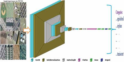
Therefore, the objective of this study is to apply the deep CNN-FE approach built from scratch for LCLU classification in RS images and improve the state-of-the-art baseline study performances. Moreover, approving the developed model in the cases of developing the DL pre-trained network and retraining the developed model on the other RS dataset is another objective of this paper. To achieve these objectives, we preprocessed the datasets and trained the model with 17 layers (four Conv2D, four-batch normalization, four pooling, one dropout, one flatten, three dense including the output (softmax) at the top) as figured in Figure 1. Finally, we evaluated the model with test set samples and compared the results from the state-of-the-art baseline studies and the VGG19 pre-trained model, as described in section 4.

Figure 1. Structure of CNN-FE model.

Our significant contributions to this paper are:

1. The significance of applying the DL method, CNN-FE, for the LCLU classification problem using the UC-Merced RS dataset from scratch development using the convolutional feature extractor, early stopping technique, and hyperparameters regularizations;

2. Evaluating and comparing the performance of the CNN-FE model using evaluating metrics and improving the state-of-the-art baseline studies performance in the target UC-Merced dataset; and

3. Approving the CNN-FE model by comparing its performance in building the VGG19 pre-trained model and retraining the CNN-FE model in another dataset called SIRI-WHU, which has different properties from the target UC-Merced dataset.

Related Work

LCLU contains dynamic sources of information on the observed earth surfaces because the nature of RS images is very complex. The LCLU classification in RS images has been a recent comprehensive study area (Dong et al. 2020). The deep CNNs could be applied to various domains in RS imagery data. RS image classifications (Chen, Hu, and Duan 2019; Helber et al. 2019; Huang, Wang, and Li 2019; Liang, Deng, and Zeng 2020; Stivaktakis, Tsagkatakis, and Tsakalides 2019), and object detections (Hou et al. 2019; Hu et al. 2019; Long et al. 2017; Pang et al. 2019) are some of such applications. RS image classification is one of the application domains in computer vision (Shabbir et al. 2021). This is a challenging problem in large datasets with many classes and different conditions (Alhichri et al. 2021). Moreover, DL models are also powerful for validating feature extraction capabilities in computer vision (Gong et al. 2022). Thus, we propose DL methods for this challenging problem, which needs more investigation.

Despite the prominent results of deep CNNs, there are some problems to be solved regarding selecting fit hyperparameters and dataset sampling. Recent studies have shown that varying the hyperparameters affects the model’s performance, such as (Long et al. 2017; Zheng et al. 2022). These hyperparameters, the kernel size (Chen, Hu, and Duan 2019; Peng et al. 2019), dropout (Li, Zhang, and Zhu 2019; Stivaktakis, Tsagkatakis, and Tsakalides 2019), and learning rate (Li, Zhang, and Zhu 2019; Long et al. 2017; Zhang et al. 2020), could affect the performance and produce different performance results. In addition to the DL hyperparameters, studies such as (Bosco, Wang, and Hategekimana 2021; Helber et al. 2019; Liang, Deng, and Zeng 2020; Zhang et al. 2020) have also tried to investigate the influences of the train-test dataset splitting percentages on the CNN models by differentiating train-test sampling sizes. In general, using various hyperparameters influences the DL model performances. Thus, we incorporated such reliable hyperparameters with their valuable values in this paper.

As we explained in the introduction section earlier, many researchers have tried to investigate the DL methods using pre-trained feature extraction architecture. Nevertheless, very few studies, such as those (Helber et al. 2019; Stivaktakis, Tsagkatakis, and Tsakalides 2019), have tried to create CNN models in RS image classification from scratch.

The study (Stivaktakis, Tsagkatakis, and Tsakalides 2019) has studied the CNN model by focusing on data augmentation and dropout hyperparameters and training the model in 1600 training sets, and testing the performance of the model in 500 test sets. However, this study’s sigmoid activation function and binary-cross-entropy loss function could influence the performance since these hyperparameters are recommended for binary classification rather than multiclass classifications, as the UC-Merced dataset is a multiclass classification problem. As we observed from the reviewed literature, the DL hyperparameters significantly influence the model’s performance.

The study (Helber et al. 2019) has also investigated the Bag-of-Visual-Words (BoVW), CNN (with three layers), ResNet-50, and GoogleNet models by varying the training-test split set ratio starting from 10/90 to 90/10 on EuroSAT, UC-Merced, AID, Sat-6 and BCS dataset. Still, the hyperparameter optimization technique is required to increase the CNN model performance that is built from scratch. We took only the CNN model accuracy result trained on the UC-Merced dataset for performance comparison in our paper, as shown in Table 8.

Thus, considering these state-of-the-art studies’ limitations, we built the CNN-FE model from scratch to LCLU classification in RS images and compared its performance with state-of-the-art studies. To fight over-fitting and increase the CNN-FE performance, we deployed new optimal regularizations and early stopping techniques implemented in this paper, as shown in Table 1.

Materials and Methods

This paper proposed to build the CNN-based feature extraction (CNN-FE) method from scratch for the LCLU classification problem in the inconsistent RS images using various DL layers, as shown in Figure 1. To compare the performance and approve the applicability of the CNN-FE model, we built the VGG19 pre-trained model. We have used two datasets, namely, the UC-Merced dataset, which is our target dataset for building the model, and the SIRI-WHU dataset used for model approval purposes. The DL Keras and Tensorflow open-source software were also the essential materials we used for experimental executions.

Convolutional Neural Networks

In this paper, we used the most prominent DL approach CNNs in the form of Conv2D, which took the image shape (height, width, channel), i.e. (256, 256, 3). The CNNs are multi-layer neural networks used to extract image features or pixels. The CNNs consist of convolution, pooling, and fully connected layers integrated with other DL hyperparameters. We described each sequential process for the end-to-end DL approach in the following and depicted in Figure 1.

The Input Layer and Convolutional (Conv2d) Layers

The input layer is the entire input image layer with height*width*channel pixel shapes. It is introduced into the convolutional layer to be processed. Convolutional layers then receive the input layers and image pixels. The convolutional layers compute the perceptron with a given filter (f, f), pooling, stride, and padding to transform the input image volume into a new output volume.

The CNNs can successfully capture deep spatial feature representations for RS scene classification (Zeng, Chen, and Song 2021) with convolution. The CNN convolution could operate the mathematical operation of matrix multiplications in the given layers, and every image is represented in the form of an array of values or pixels. In convolutional operations, the arrays are multiplied pixel-wise, and the product is summed to create a new array or feature map representing height_new * width_new based on Equation (1)(1) $\mathrm{h}\mathrm{e}\mathrm{i}\mathrm{g}\mathrm{h}\mathrm{t}\mathrm{\_}\mathrm{n}\mathrm{e}\mathrm{w}=\mathrm{w}\mathrm{i}\mathrm{d}\mathrm{t}\mathrm{h}\mathrm{\_}\mathrm{n}\mathrm{e}\mathrm{w}=\left[\left(\mathrm{h}\mathrm{e}\mathrm{i}\mathrm{g}\mathrm{h}\mathrm{t}\mathrm{\_}\mathrm{n}\mathrm{e}\mathrm{w}-\mathrm{f}+2\mathrm{p}\right)/\mathrm{s}\right]+1$(1) computations. The CNNs are different from other conventional ML approaches in input data types and weight calculations (Kim et al. 2018) with the convolution method. The overall process of the convolutional layers makes the model’s feature map.

The feature map of the model can be transformed into other resolution feature maps using the downsampling and upsampling techniques. The downsample is a convolution operation with strides to reduce the input image size and double the number of filters. In contrast, upsampling is a bilinear interpolation operation to double the input image size and reduce the number of filter sizes (Wang et al. 2021).

The convolutional layers consist of convolution filters or kernels with learnable parameters (Maggiori et al. 2016; Peng et al. 2019). Convolution could be performed with valid convolution (no padding), same convolution (with padding), and stride (slide or shift) convolution. The mathematical computation of the output volume of the image in each layer could be calculated using the input volume (height*width), stride(s), and padding (p) parameters. Stride (s) of the filter (f × f) is the interval of the filter jumps/shifts s number of transitions from the first elements in a pixel or each spatial dimension. At the same time, padding (p) is the number of pixels added at the outer edges of the input image volumes (height × width). A filter is usually odd, and smaller in size is 1 × 1, 3 × 3, 5 × 5, and 7 × 7 with 0, 1, 2, and 3 paddings, respectively. In the keras DL tool, there is no padding for image border (0) to valid convolution and padding for image border to same convolution. Thus, the output volume (height_new*width_new) of a layer could be computed using (1), and the number of padding for same convolution could be calculated using (2). The default values of p and s are 0 and 1, respectively.

In this paper, we use the same convolution with the filter size (3,3) and three paddings. The Conv2D layers are used to extract the input image features by sliding a convolution filter size of (3, 3) to produce a new output hierarchical feature map. There are four convolutional block layers in our sequential model training, including 64, 128, and 256 convolution kernels with a filter size of three each. The convolution activates image features using convolutional filters or kernels that denote the weight matrix. Therefore, convolution is used as our feature extraction method for RS images.

(1) $\mathrm{h}\mathrm{e}\mathrm{i}\mathrm{g}\mathrm{h}\mathrm{t}\mathrm{\_}\mathrm{n}\mathrm{e}\mathrm{w}=\mathrm{w}\mathrm{i}\mathrm{d}\mathrm{t}\mathrm{h}\mathrm{\_}\mathrm{n}\mathrm{e}\mathrm{w}=\left[\left(\mathrm{h}\mathrm{e}\mathrm{i}\mathrm{g}\mathrm{h}\mathrm{t}\mathrm{\_}\mathrm{n}\mathrm{e}\mathrm{w}-\mathrm{f}+2\mathrm{p}\right)/\mathrm{s}\right]+1$(1)

(2) $p=\left(f-1\right)/2$(2)

In the convolution process, the number of parameters (params) could be calculated with (3) and (4). The total parameter numbers of the model are the summations of the calculated results from Conv2D and Dense layers. We design the model with four Conv2D layers that calculate the number of parameters for those layers in the same norm by (3) and two dense layers (4). However, the calculation formula of dense parameters differs from Conv2D as equated in (4). Number 1 refers to the bias associated with each filter for learning.

(3) $\mathrm{C}\mathrm{o}\mathrm{n}\mathrm{v}2\mathrm{D}\mathrm{p}\mathrm{a}\mathrm{r}\mathrm{a}\mathrm{m}\mathrm{\#}=\mathrm{\#}\mathrm{o}\mathrm{u}\mathrm{t}\mathrm{p}\mathrm{u}\mathrm{t}\mathrm{c}\mathrm{h}\mathrm{a}\mathrm{n}\mathrm{n}\mathrm{e}\mathrm{l}\ast \left(\mathrm{\#}\mathrm{i}\mathrm{n}\mathrm{p}\mathrm{u}\mathrm{t}\mathrm{c}\mathrm{h}\mathrm{a}\mathrm{n}\mathrm{n}\mathrm{e}\mathrm{l}\ast \mathrm{f}\mathrm{i}\mathrm{l}\mathrm{t}\mathrm{e}\mathrm{r}\mathrm{h}\mathrm{e}\mathrm{i}\mathrm{g}\mathrm{h}\mathrm{t}\ast \mathrm{f}\mathrm{i}\mathrm{l}\mathrm{t}\mathrm{e}\mathrm{r}\mathrm{w}\mathrm{i}\mathrm{d}\mathrm{t}\mathrm{h}+1\right)$(3)

(4) $\mathrm{D}\mathrm{e}\mathrm{n}\mathrm{s}\mathrm{e}\mathrm{p}\mathrm{a}\mathrm{r}\mathrm{a}\mathrm{m}\mathrm{\#}=\mathrm{\#}\mathrm{o}\mathrm{u}\mathrm{t}\mathrm{p}\mathrm{u}\mathrm{t}\mathrm{c}\mathrm{h}\mathrm{a}\mathrm{n}\mathrm{n}\mathrm{e}\mathrm{l}\ast \left(\mathrm{\#}\mathrm{i}\mathrm{n}\mathrm{p}\mathrm{u}\mathrm{t}\mathrm{c}\mathrm{h}\mathrm{a}\mathrm{n}\mathrm{n}\mathrm{e}\mathrm{l}+1\right)$(4)

Pooling Layer

The pooling layer is used to resize and downsample the spatial representations, followed by convolutional operations. We use a common pooling technique called max pooling. Max pooling could pick the most activated feature and could be used to reduce overfitting and reduce the number of parameters.

Therefore, the pooling layers in CNNs are essential for downsampling processes used to reduce the size of the input RS images. In addition, the block layers involve various max-pooling with two, the stride with two, and the padding with “same.”

Fully Connected Layers (FCNs)

FCNs are feature classifiers in the last couple of layers of the network. They include flatten layers, dense layers, and an output layer at the end. Perceptrons in an FCN are fully connected to all activations of the previous layer.

The CNNs also have various activation functions, which should be non-linear as linear functions have a constant derivative, as described in our previous work (Alem and Kumar 2021). These are softmax, rectified linear unit (Relu), hyperbolic tangent (tanh), and sigmoid or logistic functions. We use the result at the entire convolutional layers to activate the weights in each convolution process and the softmax at the output layer since it is reliable for our multiclass classification problem. The softmax function is a feature classifier, and it introduces a probability score for each class. The highest probability score among each class is predicted as our predicted class. This probability score will be used for performance evaluations in section 4.

Dataset Descriptions

The RS dataset has been collected through advanced sensor technologies, and then they could label manually for research or other commercial purposes. We used the common UC-Merced dataset and the rarely investigated SIRI-WHU dataset to check the possible applicability of the built model on the target UC-Merced. We divided both datasets into 60%, 20%, and 20% for training, validation, and tasting samples for each labeled class.

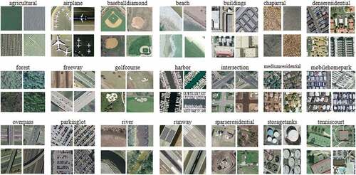
The UC-Merced dataset is an LCLU data set collected from the earth, labeled manually, and introduced by (Yang and Newsam 2010). It contains 21 classes with 100 images each, measuring 256 × 256 pixels with a spatial resolution of about 30 cm per pixel. However, the UC-Merced dataset is inconsistent as about 44 images have different pixel shapes. The variety of properties of the dataset could affect the performance results. Sample images in each class are depicted in Figure 2. This dataset is available at http://weegee.vision.ucmerced.edu/datasets/landuse.html.

Figure 2. Sample images in each classes of the UCM dataset.

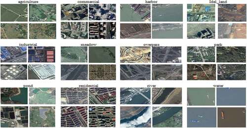
The SIRI-WHU dataset was collected from Google Earth that covered urban areas in China, and it was introduced by (Zhao et al. 2016). The dataset contains 12 categories and 200 images per category with 200 × 200 pixels in a spatial resolution of 200 cm per pixel. Sample images in each category are depicted in Figure 3. The dataset is publicly available for research purposes at https://figshare.com/articles/dataset/SIRI_WHU_Dataset/8796980.

Figure 3. Sample images in each class of the SIRI-WHU dataset used for CNN-FE model checking.

Experimental Results and Discussions

Our experiment was executed with an Intel Core i3-4000 M CPU 2.40 GHz RAM = 4GB laptop personal computer integrated with the Collaboratory on its Tesla T4 GPU. Keras and Tensorflow open-source DL software packages were used for this experiment.

Experimental Setting

The dataset and the DL hyperparameters could be considered for their appropriate settings to build our model. As we described in section 3.2, there are 2100 images in the UC-Merced dataset and 2400 images in the SIRI-WHU dataset. Therefore, to reduce the overfitting of the model, we split both the UC-Merced and SIRI-WHU datasets into three sets: training set, validation set, and test set in 60%, 20%, and 20% of the dataset, respectively. Then after splitting, the total sample images in the training set, validation set, and test set becomes 1260, 420, and 420 for UC-Merced and 1440, 480, and 480 for SIRI-WHU, respectively. Each dataset is loaded into the experiment and preprocessed. First, we built the model on the UC-Merced dataset as follows: then, we rebuilt the model on the SIRI-WHU dataset for its applicability approval in the same manner.

The training set is a collection of 1260 images that have been used to fit and train our model with a batch size of 64 and hundreds of epochs, as shown in Table 1 (right column). In each epoch, the same training images are fed to CNN-FE architecture recurrently, and the model could learn and continue to learn from the hidden image features. In general, the model has been trained on a training set in four CNNs sequential layers and its performance has been evaluated with the validation set during the training and with test set after the training.

The validation set is a collection of 420 images separate from the training set that was used to validate our model performance during the training. Splitting the dataset into a validation set is critical in reducing the overfitting of training and evaluating the model during its development.

On the other hand, the test set is a set of 420 images used to evaluate the performance of our model after completing the training. The test set is the support as shown in the last column of Tables 2–5. It is used to analyze the performance evaluation metrics, including accuracy, loss, precision, recall, F1-score, and confusion matrix, as we described in section 4.2.

Table 2. Summarization of the classification performance of CNN-FE for each class with performance measurement metrics in the UC-Merced dataset.

Class name	Precision	Recall	F1-score	Support
Agricultural	0.91	1.00	0.95	20
Airplane	0.94	0.80	0.86	20
Baseballdiamond	0.85	0.85	0.85	20
Beach	0.95	1.00	0.98	20
Buildings	0.79	0.75	0.77	20
Chaparral	1.00	0.95	0.97	20
Denseresidential	0.57	0.80	0.67	20
Forest	0.86	0.95	0.90	20
Freeway	0.95	0.90	0.92	20
Golfcourse	0.80	0.60	0.69	20
Harbor	0.91	1.00	0.95	20
Intersection	0.88	0.75	0.81	20
Mediumresidential	0.58	0.90	0.71	20
Mobilehomepark	0.92	0.55	0.69	20
Overpass	0.81	0.85	0.83	20
Parkinglot	1.00	0.85	0.92	20
River	0.78	0.90	0.84	20
Runway	0.95	0.90	0.92	20
Sparseresidential	0.75	0.90	0.82	20
Storagetanks	1.00	0.90	0.95	20
Tenniscourt	1.00	0.70	0.82	20

Table 3. Summarizations of the classification performance of VGG19 for each class in performance measurement metrics in the UC-Merced dataset.

Class name	Precision	Recall	F-score	Support
Agricultural	1.00	1.00	1.00	20
Airplane	0.95	0.90	0.92	20
Baseballdiamond	1.00	0.90	0.95	20
Beach	1.00	0.95	0.97	20
Buildings	0.82	0.70	0.76	20
Chaparral	1.00	1.00	1.00	20
Denseresidential	0.50	0.55	0.52	20
Forest	0.82	0.90	0.86	20
Freeway	1.00	0.85	0.92	20
Golfcourse	0.86	0.60	0.71	20
Harbor	1.00	1.00	1.00	20
Intersection	0.81	0.85	0.83	20
Mediumresidential	0.69	0.90	0.78	20
Mobilehomepark	0.61	0.55	0.58	20
Overpass	0.84	0.80	0.82	20
Parkinglot	0.95	0.95	0.95	20
River	0.76	0.95	0.84	20
Runway	0.87	1.00	0.93	20
Sparseresidential	0.90	0.90	0.90	20
Storagetanks	0.95	0.95	0.95	20
Tenniscourt	0.85	0.85	0.85	20

Table 4. Summarizations the classification performance of CNN-FE for each individual class with performance measurement metrics in SIRI-WHU dataset.

Class name	Precision	Recall	F1-score	Support
Agriculture	0.81	0.65	0.72	40
Commercial	0.94	0.82	0.88	40
Harbor	0.88	0.75	0.81	40
Idle_land	0.62	0.78	0.69	40
Industrial	0.90	0.90	0.90	40
Meadow	0.55	0.60	0.57	40
Overpass	0.92	0.90	0.91	40
Park	0.79	0.68	0.73	40
Pond	0.72	0.82	0.77	40
Residential	0.83	0.95	0.88	40
River	0.81	0.75	0.78	40
Water	0.93	1.00	0.96	40

Table 5. Summarizations of the classification performance of VGG19 for each class with performance measurement metrics in the SIRI-WHU dataset.

Class name	Precision	Recall	F1-score	Support
Agriculture	0.91	0.50	0.65	40
Commercial	0.72	0.95	0.82	40
Harbor	0.88	0.93	0.90	40
Idle_land	0.86	0.62	0.72	40
Industrial	0.85	0.88	0.86	40
Meadow	0.63	0.60	0.62	40
Overpass	0.80	0.97	0.88	40
Park	0.50	0.60	0.55	40
Pond	0.67	0.75	0.71	40
Residential	0.92	0.88	0.90	40
River	0.85	0.72	0.78	40
Water	0.98	1.00	0.99	40

In addition to setting the dataset splitting, we have chosen the DL hyperparameters to build, compile, and fit our model on the UC-Merced dataset and evaluate the model’s performance as shown in Table 1. Both dropout and early stopping hyperparameters are used for reducing over-fitting. Early stopping is a technique that could automatically stop the training when either validation loss has stopped decreasing or validation accuracy has stopped increasing. In addition to these techniques, the convolutional techniques were applied to preprocess and extract feature maps by reducing the image shape (256, 256, 3) into other reduced feature maps.

Performance Evaluation Metrics and Experimental Results

After validating the model using the validation set during training, we retrained it by combining the training set and validation set with an early stopping technique. Hereafter, the training set sample images become 80% of the dataset for validating the model’s performances with 20% of the test set sample images.

After building the model, we evaluated its performance using the evaluation measurement metrics of accuracy, precision, recall, F1-score, and confusion or error matrix (CM). In addition to these evaluation metrics, we used the loss function, i.e., the categorical_cross_entropy, to evaluate the training and validation errors. The training losses are calculated during each epoch, whereas validation losses are computed after each training epoch for the errors. At most, when the number of epochs increases, the losses decrease, and the accuracies increase.

The model’s accuracy was evaluated in two ways, i.e., with and without using the early stopping technique. The early stopping has been stopped at a random iteration epoch from out of 100 epochs when either the validation accuracy has been stopped increasing (as depicted in Figures 4b, 5b, 6b, and 7b) or the validation loss stopped decreasing (as depicted in Figures 8b, 9b, 10b, and 11b) while evaluating the models with test set sample images. Therefore, from the experiments with and without early stopping, we observed that the accuracy result increased using the early stopping technique in each model of CNN-FE and VGG19 trained on both datasets, as shown in Table 7.

Figure 4. Training and validation accuracies with and without applying early stopping technique. (a) Before applying early stopping. (b) After applying early stopping.

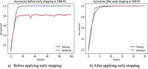
Figure 5. Training and validation accuracies in VGG19 with and without applying early in stopping technique in UC-Merced dataset. (a) Before applying early stopping. (b) After applying early stopping.

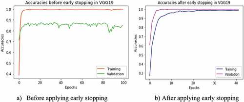
Figure 6. Training and validation accuracies of CNN-FE model in SIRI-WHU dataset with and without applying early stopping technique. (a) Before applying early stopping. (b) After applying early stopping.

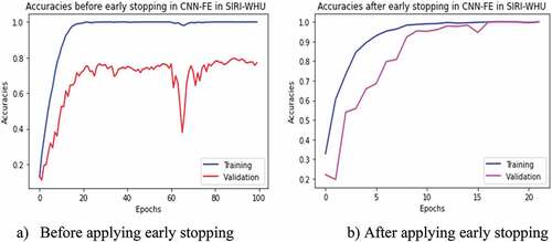
Figure 7. Training and validation accuracies of VGG19 in the SIRI-WHU dataset with and without applying the early stopping technique. (a) Before applying early stopping. b) After applying early stopping.

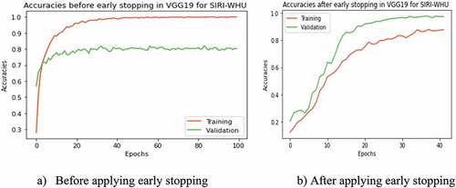
Figure 8. Training and validation losses with and without applying early stopping technique. (a) Losses before applying early stopping. (b) Losses after applying early stopping.

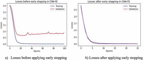
Figure 9. Training and validation losses in VGG19 with and without applying the early stopping technique in the UC-Merced dataset. (a) Before applying early stopping. b) After applying early stopping.

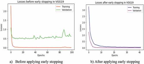
Figure 10. Training and validation losses of CNN-FE model in SIRI-WHU dataset with and without applying early stopping technique. (a) Before applying early stopping. (b) After applying early stopping.

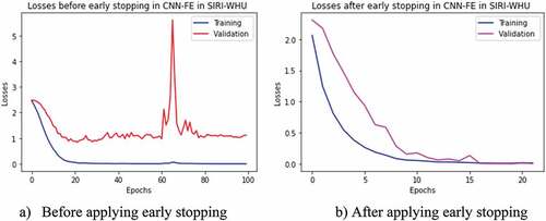
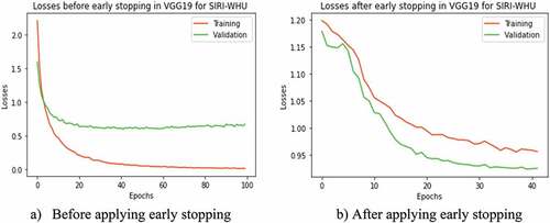
Figure 11. Training and validation losses of VGG19 in SIRI-WHU dataset with and without applying early stopping technique. (a) Before applying early stopping. (b) After applying early stopping.

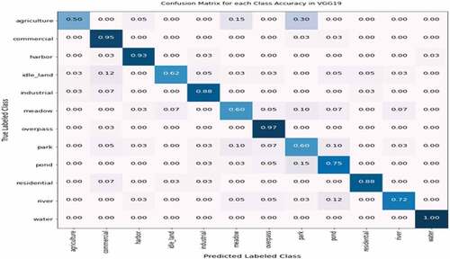
In addition to evaluating the overall accuracy of both models, we assessed each class with 20 sample images per class using precision, recall, and F1-score performance measurement merits as stated in Tables 2–5. Furthermore, the CM metric was also used to identify the predicted classes based on the higher normalized probability values in each class intersection. CM considers the normalized probability values for each class category in rows (True labeled class) and columns (predicted labeled class), as shown in Figures 12–15. CM measures the performance of the DL model, whether each class is correctly classified or incorrectly classified. Therefore, according to Figures 12–15, the score in the diagonal intersection showed the correct classified classes with higher normalized probability. In contrast, the results in other rows-columns wise are predicted in misclassified classes with lower normalized probability.

Figure 12. CM performance results in the CNN-FE model for each labeled class.

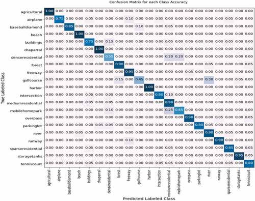
Figure 13. CM performance results of VGG19 pre-trained for each labeled class.

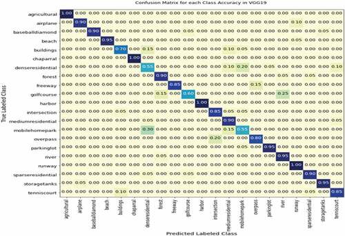
Figure 14. CM performance results of CNN-FE for each class classification in SIRI-WHU.

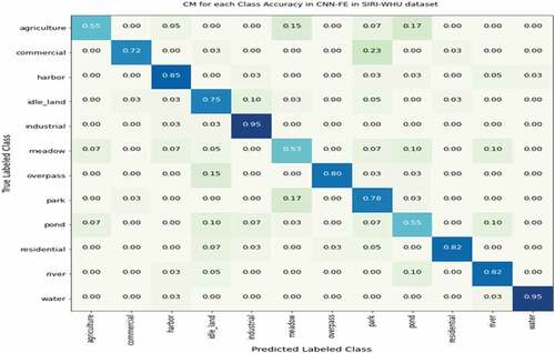
Figure 15. CM performance results of VGG19 for each class classification in SIRI-WHU.

Model Validations with VGG19 Pre-Trained Network and SIRI-WHU Dataset

After building and evaluating the CNN-FE model, we assured its possible applicability to the LCLU classification in RS images by comparing its performance with the VGG19 feature extractor network and retrained on another dataset called SIRI-WHU.

The VGG19 pre-trained feature extractor was trained on the pre-trained network, which was trained on the large dataset “imagenet” in the same hyperparameters to check the applicability of CNN-FE for LCLU classification in RS images. The VGG19 was designed by (Simonyan and Zisserman 2015) to analyze the neural network depth effect on the accuracy of image recognition. Therefore, we created the VGG19 pre-trained model to compare its performance with CNN-FE trained on UC-Merced and SIRI-WHU. While comparing the accuracy performances of both DL models, CNN-FE outperformed VGG19 as compared in Table 7. Using the early stopping technique improved the accuracy performance of VGG19 in both datasets as CNN-FE, as shown in Table 7.

In addition to checking its applicability on the other DL pre-trained model, we retrained the CNN-FE model on the SIRI-WHU dataset. As we stated earlier, the properties of the dataset could influence the performance of DL models. We used the SIRI-WHU dataset with different properties from the target dataset UC-Merced to see this effect. After training the CNN-FE model on the SIRI-WHU dataset, the validation accuracy and loss fluctuated, especially between epochs 60 and 80 than the validation accuracy and loss trained in UC-Merced, as shown in Figures 6a and 10a.

Discussions

This study investigated the application of an end-to-end DL approach called CNN-FE for LCLU classification using RS images. We showed the possibility of designing CNNs from scratch to develop LCLU classification in complex RS images using two different datasets. We also developed a comparative VGG19 pre-trained network using the same hyperparameters. In addition to validating this DL pre-trained model, we retrained the CNN-FE on the SIRI-WHU dataset and assured its applicability in the domain area. Therefore, as far as our knowledge, CNN-FE is significant in this study.

Discussions on Results

The CNN-FE model performance result indicates the possibility of building the DL models from scratch. It is comparable to those trained from pre-trained models in the UC-Merced dataset. Significant results were reported when compared with VGG19 pre-trained architecture. In addition, the CNN-FE was retrained on the SIRI-WHU dataset, and a considerable accuracy performance was achieved in the UC-Merced, as shown in Table 7. To sum up, the performance of the CNN-FE model resulting from various measurement metrics showed that it is possible to prove its applicability to the classification problem in RS images.

Each class classification performance was evaluated with precision, recall, and F1-score. Therefore, according to Table 2, the classes such as chaparral, parking lot, storage tanks and tennis court have the best precision performed, which means that these classes were precisely predicted. However, the lower result precisions were reported in dense residential (i.e., 0.57), which means that it has inflexible properties to predict precisely. The classes such as agricultural beach and harbor were classified in best recall performance, whereas mobile homepark class scored the lower recall performance. Classes with the perfect or lower performance in both precision and recall are also the perfect or lower results in F1-score. Thus, there were no same classes with perfect or lower performance in both metrics, and there were no perfect classes in F1-score. However, a lower F1-score was recorded in dense residential (0.67) class. Perfect performance means 100% accurately and precisely classified when measured in given metrics.

To sum up, the individual class performance of the two models in the two datasets is summarized in Table 6. The dense residential class has lower performance in both methods than other classes in the UC-Merced dataset, while the meadow and park classes have lower performance in CNN-FE and VGG19, respectively, in the SIRI-WHU dataset. In the case of CM metrics, better result performance for each class has been observed in both methods in the UC-Merced dataset than in the SIRI-WHU dataset, as compared and shown in Figures 12–15.

Table 6. Class comparisons in precision, recall, and F1-score (%) on the two models and datasets.

Dataset	Method	Precision performance		Recall performance		F1-score performance
		Perfect (1) classes	Lower (-) classes	Perfect (1) classes	Lower (-) classes	Perfect (1) classes	Lower (-) classes
UC-Merced	CNN-FE	Chaparral, parkinglot, storagetanks, and tenniscour	Denseresidential (0.57)	Agricultural, beach and harbor	Mobilehomepark (0.55) and golfcourse (0.60)	None	Denseresidential (0.67)
	VGG19	Agricultural, baseballdiamond, beach, charparral, freeway, and harbor	Denseresidential (0.50)	Agricultural, charparral, harbor and runway	Denseresidential (0.55)	Agricultural, charparral, and harbor	Denseresidential (0.52)
SIRI-WHU	CNN-FE	None	Meadow (0.55)	Water	Meadow (0.60)	None	Meadow (0.57)
	VGG19	None	Park (0.50)	Water	Agriculture	None	Park (0.55)

The classes, such as agricultural, harbor, overpass, and river, are common in both datasets. However, most of these classes have different performance values, as shown in Tables 2–6. This could be why the two datasets have inconsistent properties, which were collected from different locations with different resolutions and pixel values.

In addition to evaluating the individual classes, we also evaluated the two methods within the two datasets. Thus, while comparing the CNN-FE from the pre-trained VGG19 network outperformed results in CNN-FE have been achieved in both datasets, as shown in Table 7.

Table 7. Results of accuracy (%) performances at random early stopping technique.

Dataset	Methods	Stopped at epoch # out of 100	Accuracy performance results
			Before early stopping	After early stopping
UC-Merced	CNN-FE	26	85.95	89.76
	VGG19	42	85.00	85.95
SIRI-WHU	CNN-FE	22	78.67	80.00
	VGG19	41	76.88	78.33

Discussions on Similar Studies

In this paper, we aimed to improve the performance of the DL model from the existing state-of-the-art studies studied by Stivaktakis, Tsagkatakis, and Tsakalides (2019) and Helber et al. (2019) by considering their limitations of the DL hyperparameters. The DL hyperparameters influence the DL model performances. Therefore, to see the effect, we used various hyperparameters, such as dropout, learning rate, batch size, epochs, and early stopping, with their valuable values as stated in section 4.1. The study (Stivaktakis, Tsagkatakis, and Tsakalides 2019) has analyzed the dropout hyperparameter effects on the CNN performance with different values (null, 0.25, 0.50, and 0.75), which generates the accuracy of 81.2, 81.3, 81.4, and 79.7 with augmentation and 68.0, 73.7, 75.7, and 77.7 without data augmentation technique, respectively. Among these provided accuracies and dropout values, we listed and compared the last two accuracy performances with unaugmented data with corresponding dropout values of 0.5 and 0.75, respectively, shown in Table 8. The CNN-FE model has achieved 89.76% and 80% accuracy in the UC-Merced and the SIRI-WHU dataset, respectively. The VGG19 pre-trained model has also achieved 85.95% and 78.33% accuracy, as shown in Table 7. Moreover, the CNN-FE model outperformed the state-of-the-art studies and the pre-trained network, as shown in Table 8.

Table 8. General comparison of the accuracy (%) with the state-of-the-arts in the UC-Merced target dataset.

Method	Dropout	Precision	Recall	F1-score	Accuracy
CNNs (Radamanthys Stivaktakis, Tsagkatakis, and Tsakalides 2019)	0.50	85.4	83.3	84.3	75.7
	0.75	85.5	85.8	85.7	77.7
CNN (Helber et al. 2019)	-	-	-	-	82.38
CNN-FE (Ours)	0.50	90.00	88.00	88.99	89.76
VGG19 (Ours)	0.50	88.00	86.00	86.99	85.95

Conclusion

In this paper, we have applied the CNN-FE model built from scratch to address the challenge of LCLU classification in RS images. Although CNNs are powerful DL approaches to analyzing RS images for LCLU classification systems, designing CNN models from scratch has not been solved yet. It is crucial to build CNN models from scratch for RS images since RS images are inconsistent, and modeling them from pre-trained networks could affect the result.

Therefore, we applied an end-to-end CNN-FEDL model to extract the inconsistent UC-Merced RS image features for LCLU classification in RS images. We retrained this model on the other SIRI-WHU dataset to analyze whether the dataset influences the model performance. We also built a VGG19 pre-trained DL model on both datasets and evaluated their performances to validate the CNN-FE possible applicability in the domain area. We compare its result with the state-of-the-art earlier studies and the VGG19 pre-trained model, trained in the same hyperparameters. The CNN-FE outperformed the accuracy performance from state-of-the-art earlier studies and the VGG19 Pre-trained model. Therefore, we proved that the developed CNN-FE model is possibly applicable to the domain area and improved performance. However, the model needs more improvements, validations, and comparisons with other traditional machine learning approach in large datasets. Therefore, building DL and traditional ML approaches in other large RS datasets is our future task to compare their performances.

Acknowledgments

The Ethiopian Ministry of Education (MoE), cooperatively with Debre Tabor University, has provided a monthly stipend for this paper. Reviewing a manuscript is a challenging task in which the editors and reviewers share their deep and experienced knowledge with different authors from various disciplines. Therefore, we authors would like to thank the anonymous editors and reviewers of the Applied Artificial Intelligence International Journal (E-ISSN: 1087-6545) for their constructive reviews and comments by devoting their precious time to improving this quality paper.

Disclosure statement

No potential conflict of interest was reported by the author(s).

References

- Alem, A., and S. Kumar. 2021. Transfer learning models for land cover and land use classification in remote sensing image. Applied Artificial Intelligence 36 :2014192. doi:10.1080/08839514.2021.2014192.
- Alhichri, H., A. S. Alswayed, Y. Bazi, N. Ammour, and N. A. Alajlan. 2021. Classification of remote sensing images using EfficientNet-B3 CNN model with attention. IEEE Access 9 ():14078–3328. doi:10.1109/ACCESS.2021.3051085.
- Bahri, A., S. G. Majelan, S. Mohammadi, M. Noori, and K. Mohammadi. 2020. Remote Sensing Image Classification via Improved Cross-Entropy Loss and Transfer Learning Strategy Based on Deep Convolutional Neural Networks. IEEE Geoscience and Remote Sensing Letters 17 (6):1087. doi:10.1109/LGRS.2019.2937872.
- Bosco, M. J., G. Wang, and Y. Hategekimana. 2021. Learning multi-granularity neural network encoding image classification using DCNNs for easter Africa community countries. IEEE Access 9 ():146703–18. doi:10.1109/ACCESS.2021.3122569.
- Cheng, G., Z. Li, X. Yao, L. Guo, and Z. Wei. 2017. Remote sensing image scene classification using bag of convolutional features. IEEE Geoscience and Remote Sensing Letters 14 (10):1735–39. doi:10.1109/LGRS.2017.2731997.
- Chen, D., P. Hu, and X. Duan. 2019. Complex scene classification of high resolution remote sensing images based on DCNN model. 2019 10th International Workshop on the Analysis of Multitemporal Remote Sensing Images (MultiTemp), 1–4. 10.1109/Multi-Temp.2019.8866895
- Chen, Y., Y. Wang, Y. Gu, X. He, P. Ghamisi, and X. Jia. 2019. Deep learning ensemble for hyperspectral image classification. IEEE Journal of Selected Topics in Applied Earth Observations and Remote Sensing 12 (6):1882–97. doi:10.1109/JSTARS.2019.2915259.
- Dong, S., Y. Zhuang, Z. Yang, L. Pang, H. Chen, and T. Long. 2020. Land cover classification from VHR optical remote sensing images by feature ensemble deep learning network. IEEE Geoscience and Remote Sensing Letters 17 (8):1396–400. doi:10.1109/LGRS.2019.2947022.
- Du, P., E. Li, J. Xia, A. Samat, and X. Bai. 2019. Feature and model level fusion of pretrained CNN for remote sensing scene classification. IEEE Journal of Selected Topics in Applied Earth Observations and Remote Sensing 12 (8):2600–11. doi:10.1109/JSTARS.2018.2878037.
- Fan, R., R. Feng, L. Wang, J. Yan, and X. Zhang. 2020. Semi-MCNN: A semisupervised multi-CNN ensemble learning method for urban land cover classification using submeter HRRS images. IEEE Journal of Selected Topics in Applied Earth Observations and Remote Sensing 13:4973–87. doi:10.1109/JSTARS.2020.3019410.
- Gong, N., C. Zhang, H. Zhou, K. Zhang, Z. Wu, and X. Zhang. 2022. Classification of hyperspectral images via improved cycle‐MLP. Institutions of Engineering and Technology Computer Vision 16 (5):468–78. doi:10.1049/cvi2.12104.
- Helber, P., B. Bischke, A. Dengel, and D. Borth. 2019. Eurosat: A novel dataset and deep learning benchmark for land use and land cover classification. IEEE Journal of Selected Topics in Applied Earth Observations and Remote Sensing 12 (7):2217–26. doi:10.1109/JSTARS.2019.2918242.
- Hou, B., J. Li, X. Zhang, S. Wang, and L. Jiao (2019). Object detection and tracking based on convolutional neural networks for high-resolution optical remote sensing video. IGARSS 2019 - 2019 IEEE International Geoscience and Remote Sensing Symposium, 5433–36. 10.1109/IGARSS.2019.8898173
- Huang, W., Q. Wang, and X. Li (2019). Feature sparsity in convolutional neural networks for scene classification of remote sensing image school of computer science and center for optical imagery analysis and learning (OPTIMAL). IGARSS 2019 - 2019 IEEE International Geoscience and Remote Sensing Symposium, 3017–20. 10.1109/IGARSS.2019.8898875
- Hu, Y., X. Li, N. Zhou, L. Yang, L. Peng, and S. Xiao. 2019. A sample update-based convolutional neural network framework for object detection in large-area remote sensing images. IEEE Geoscience and Remote Sensing Letters 16 (6):947–51. doi:10.1109/LGRS.2018.2889247.
- Kang, W., Y. Xiang, F. Wang, and H. You. 2022. DO-net : Dual-output network for land cover classification from optical remote sensing images. IEEE Geoscience and Remote Sensing Letters 19 (Art no. 8021205):1–5. doi:10.1109/LGRS.2021.3114305.
- Kim, M., J. Lee, D. Han, M. Shin, J. Im, J. Lee …, and L. J. Quackenbush, Z. Gu. 2018. Convolutional neural network-based land cover classification using 2-D spectral reflectance curve graphs with multitemporal satellite imagery. IEEE Journal of Selected Topics in Applied Earth Observations and Remote Sensing 11 (12):4604–17. doi:https://doi.org/10.1109/JSTARS.2018.2880783.
- Liang, J., Y. Deng, and D. Zeng. 2020. A deep neural network combined CNN and GCN for remote sensing scene classification. IEEE Journal of Selected Topics in Applied Earth Observations and Remote Sensing 13:4325–38. doi:10.1109/JSTARS.2020.3011333.
- Lin, P., M. Sun, C. Kung, and T. Chiueh. 2019. FloatSD : A new weight representation and associated update method for efficient convolutional neural network training. IEEE Journal on Emerging and Selected Topics in Circuits and Systems 9 (2):267–79. doi:10.1109/JETCAS.2019.2911999.
- Li, B., W. Su, H. Wu, R. Li, W. Zhang, W. Qin, S. Zhang, and J. Wei. 2020. Further Exploring Convolutional Neural Networks’ Potential for Land-Use Scene Classification. IEEE Geoscience and Remote Sensing Letters 17 (10):1687–91. doi:https://doi.org/10.1109/LGRS.2019.2952660.
- Liu, X., Y. Zhou, J. Zhao, R. Yao, B. Liu, and Y. Zheng. 2019. Siamese convolutional neural networks for remote sensing scene classification. IEEE Geoscience and Remote Sensing Letters 16 (8):1200–04. doi:10.1109/LGRS.2019.2894399.
- Li, Y., Y. Zhang, and Z. Zhu (2019). Learning deep networks under noisy labels for remote sensing image scene classification. IGARSS 2019 - 2019 IEEE International Geoscience and Remote Sensing Symposium, 3025–28. 10.1109/IGARSS.2019.8900497
- Long, Y., Y. Gong, Z. Xiao, and Q. Liu. 2017. Accurate object localization in remote sensing images based on convolutional neural networks. IEEE Transactions on Geoscience and Remote Sensing 55 (5):2486–98. doi:10.1109/TGRS.2016.2645610.
- Maggiori, E., Y. Tarabalka, G. Charpiat, and P. Alliez (2016). Fully convolutional neural networks for remote sensing image classification. 2016 IEEE International Geoscience and Remote Sensing Symposium (IGARSS), 5071–74. 10.1109/IGARSS.2016.7730322
- Mateen, M., J. Wen, Nasrullah, S. Song, and Z. Huang. 2019. Fundus image classification using VGG-19 architecture with PCA and SVD. Symmetry 11 (1):1. doi:10.3390/sym11010001.
- Nogueira, K., O. A. B. Penatti, and J. A. D. Santos. 2016. Towards better exploiting convolutional neural networks for remote sensing scene classification. Pattern Recognition 61:539–56. doi:10.1016/j.patcog.2016.07.001.
- Pang, J., C. Li, J. Shi, Z. Xu, and H. Feng. 2019. R2-CNN: Fast tiny object detection in large-scale remote sensing images. IEEE Transactions on Geoscience and Remote Sensing 57 (8):5512–24. doi:10.1109/TGRS.2019.2899955.
- Peng, C., Y. Li, L. Jiao, Y. Chen, and R. Shang. 2019. Densely based multi-scale and multi-modal fully convolutional networks for high-resolution remote-sensing image semantic segmentation. IEEE Journal of Selected Topics in Applied Earth Observations and Remote Sensing 12 (8):2612–26. doi:10.1109/JSTARS.2019.2906387.
- Qian, Y., W. Zhou, W. Yu, L. Han, W. Li, and W. Zhao. 2020. Integrating backdating and transfer learning in an object-based framework for high resolution image classification and change analysis. Remote Sensing 12 (24):4094. doi:10.3390/rs12244094.
- Russakovsky, O., J. Deng, H. Su, J. Krause, S. Satheesh, S. Ma, Z. Huang, A. Karpathy, A. Khosla, M. Bernstein, and A. C. Berg. 2015. ImageNet large scale visual recognition challenge. International Journal of Computer Vision 115 (3):211–52. doi:https://doi.org/10.1007/s11263-015-0816-y.
- Sang, Q., Y. Zhuang, S. Dong, G. Wang, and H. Chen. 2020. FRF-Net : Land cover classification from large-scale VHR optical remote sensing images. IEEE Geoscience and Remote Sensing Letters 17 (6):1057–61. doi:10.1109/LGRS.2019.2938555.
- Scott, G. J., M. R. England, W. A. Starms, R. A. Marcum, and C. H. Davis. 2017. Training deep convolutional neural networks for land-cover classification of high-resolution imagery. IEEE Geoscience and Remote Sensing Letters 14 (4):549–53. doi:10.1109/LGRS.2017.2657778.
- Senecal, J. J., J. W. Sheppard, and J. A. Shaw (2019). Efficient convolutional neural networks for multi-spectral image classification. 2019 International Joint Conference on Neural Networks (IJCNN), 14-19 July 2019, 1–8. 10.1109/IJCNN.2019.8851840
- Shabbir, A., N. Ali, J. Ahmed, B. Zafar, A. Rasheed, M. Sajid, A. Ahmed, and S. H. Dar. 2021. Satellite and Scene image classification based on transfer learning and fine tuning of ResNet50. Mathematical Problems in Engineering 2021:1–18. doi:https://doi.org/10.1155/2021/5843816.
- Shao, Z., K. Yang, and W. Zhou. 2018. Performance evaluation of single-label and multi-label remote sensing image retrieval using a dense labeling dataset. Remote Sensing 10 (6):964. doi:10.3390/rs10060964.
- Simonyan, K., and A. Zisserman. 2015. Very deep convolutional networks for large-scale image recognition ArXiv:1409.1556v6 doi:10.48550/arXiv.1409.1556.
- Stivaktakis, R., G. Tsagkatakis, and P. Tsakalides. 2019. Deep learning for multilabel land cover scene categorization using data augmentation. IEEE Geoscience and Remote Sensing Letters 16 (7):1031–1035. doi:10.1109/LGRS.2019.2893306.
- Wang, J., Y. Zhong, Z. Zheng, A. Ma, and L. Zhang. 2021. Rsnet: The search for remote sensing deep neural networks in recognition tasks. IEEE Transactions on Geoscience and Remote Sensing 59 (3):2520–34. doi:10.1109/TGRS.2020.3001401.
- Yang, Y., and S. Newsam (2010). Bag-of-visual-words and spatial extensions for land-use classification. Proceedings of the 18th SIGSPATIAL International Conference on Advances in Geographic Information Systems, 270–79. 10.1145/1869790.1869829
- Yin, X., W. Chen, X. Wu, and H. Yue (2017). Fine-tuning and visualization of convolutional neural networks. 12th IEEE Conference on Industrial Electronics and Applications (ICIEA), 1310–15. 10.1109/ICIEA.2017.8283041
- Zeng, Z., X. Chen, and Z. Song. 2021. MGFN: A multi-granularity fusion convolutional neural network for remote sensing scene classification. IEEE Access 9:76038–46. doi:10.1109/ACCESS.2021.3081922.
- Zhang, J., C. Lu, J. Wang, X.-G. Yue, S.-J. Lim, Z. Al-Makhadmeh, and A. Tolba. 2020. Training convolutional neural networks with multi ‐ size images and triplet loss for remote sensing scene classification. Sensors 20 (4):1188. doi:10.3390/s20041188.
- Zhang, Y., X. Zheng, Y. Yuan, and X. Lu. 2020. Attribute-cooperated convolutional neural network for remote sensing image classification. IEEE Transactions on Geoscience and Remote Sensing 58 (12):8358–71. doi:10.1109/TGRS.2020.2987338.
- Zhao, B., Y. Zhong, G. S. Xia, and L. Zhang. 2016. Dirichlet-derived multiple topic scene classification model for high spatial resolution remote sensing imagery. IEEE Transactions on Geoscience and Remote Sensing 54 (4):2108–23. doi:10.1109/TGRS.2015.2496185.
- Zheng, X., T. Gong, X. Li, and X. Lu. 2022. Generalized scene classification from small-scale datasets with multitask learning. IEEE Transactions on Geoscience and Remote Sensing 60:5609311. doi:10.1109/TGRS.2021.3116147.