Event-Triggered Finite-Time Tracking Control for Fractional-Order Multi-Agent Systems with Input Saturation and Constraints

ABSTRACT

This paper focuses on the finite-time tracking control problem of fractional-order multi-agent systems subject to input saturation and constraints. The interaction topology is assumed to be directed and contain a spanning tree. The appropriate barrier Lyapunov functions are constructed to tackle the output and partial states constraints. Since only the system output is available, a reduced-order state observer is constructed to obtain the unmeasurable state variables. Fuzzy logic system is applied to tackle the uncertain nonlinear dynamics in the system and the unknown parameters are estimated by adaptive laws. An event-triggered control scheme is designed to reduce communication burden. The proposed distributed controller can guarantee that all signals of the system are bounded, the constrained states never breach the time-varying constraints, finite-time tracking can be achieved with a bounded error and the Zeno behavior does not occur. At last, the effectiveness of the proposed control scheme is validated by an example.

Introduction

For a long time, most studies focus on multi-agent systems (MASs) with integer-order dynamic (Antonio et al. 2021; Chang et al. 2022; Li et al. 2022; Ma et al. 2022; Viel et al. 2022; Wang, Wang, and Huang 2022). However, fractional-order systems (FOSs) have more advantages than traditional integer-order dynamics in describing biological systems or engineering systems with memory and genetic characteristics, which makes the theory of fractional-order calculus play an irreplaceable role in the fields of information science, system control, biomedicine and so on. Therefore, the study on fractional-order MASs (FOMASs) has been widely concerned by scholars, such as containment control (Ling, Yuan, and Mo 2019; Shahamatkhah and Tabatabaei 2020; Wu et al. 2021), cluster consensus (Yaghoubi and Talebi 2020), formation control (Cajo et al. 2021; Liu, Li, Qi et al. 2019, Liu, Li, chen 2019) and so on. Compared with integer-order MASs, the study on FOMASs is still few, and the control methods of integer-order MASs cannot be applied to FOMASs directly, which makes the study of FOMASs more challenging.

In some practical applications, not only the control input but also the system state may be limited to a bounded region due to the limitations of physical devices. Therefore, it is of theoretical and practical significance to consider the control problem of constrained systems. At present, constraint problems such as input saturation (IS) (Chen et al. 2018; Fu et al. 2019, 2019, 2022; Sheng et al. 2018; Wang and Liang 2018; Wang et al. 2020), output constraints and state constraints (Wang et al. 2021; Wei, Li, and Tong 2020; Yang, Yu, and Zheng 2021) have become the main focus of engineering systems. In Wang et al. (2020), the problem of adaptive control of uncertain nonlinear incommensurate FOSs with IS based on fuzzy logic system (FLS) was considered. In Wang and Liang (2018), an neural network (NN) adaptive control method was proposed for FOSs subject to IS. The robust consensus problem of FOMASs with IS was studied in Chen et al. (2018). Taking IS into account, an adaptive backstepping control scheme with observer was proposed for FOSs in Sheng et al. (2018). In Fu et al. (2019), the consensus problem of second-order MASs with IS was considered. The robust global containment control problem for MASs subject to IS was studied in Fu et al. (2019). In Fu et al. (2022), the distributed formation navigation problem of MASs subject to IS was considered. In Yang, Yu, and Zheng (2021), the fault-tolerant fuzzy adaptive tracking control problem was investigated for uncertain nonaffine FOSs with full state constraints (FSCs), in which the barrier Lyapunov function (BLF) was applied to deal with the FSCs. In Wei, Li, and Tong (2020), an adaptive control issue for nonlinear FOSs with FSCs was addressed based on NN, and the constraint function considered was constant. Both FSCs and IS were considered in Wang et al. (2021), and an NN-based adaptive control for nonlinear FOSs was proposed.

Compared with time-triggered control, event-triggered control (ETC) (Cao and Nie 2021; Chen et al. 2020; Lin et al. 2022; Shahvali, Naghibi-Sistani, and Askari 2022; Wang and Dong 2022a, 2022b; Ye, Su, and Sun 2018; Zhang et al. 2022) can avoid unnecessary sampling and communication. The tracking control problem of FOMASs with unmeasurable states via fuzzy adaptive ETC strategy was presented in Wang and Dong (2022a). In Wang and Dong (2022b), an output feedback-based adaptive fault-tolerant fuzzy tracking control problem for FOMASs with nonlinearity and actuator failures using ETC scheme was studied. The exponential consensus problem was investigated in Zhang et al. (2022) for descriptor leader-following FOMASs with ETC protocol. In Shahvali, Naghibi-Sistani, and Askari (2022), an adaptive NN-based backstepping control scheme was designed for FOSs with nonlinearity via ETC scheme. The consensus problem of FOMASs via pinning impulsive control using ETC mechanism was studied in Lin et al. (2022). In Cao and Nie (2021), both unknown nonlinear functions and unmodeled dynamics were considered, and an adaptive NN-based ETC strategy was proposed for nonlinear FOSs with IS. In Chen et al. (2020), the consensus problem of linear leader-following FOMASs using ETC strategy in directed networks was studied. In Ye, Su, and Sun (2018), the tracking control problem of general linear FOMASs via ETC strategy was investigated.

Finite-time stability is also an important aspect in systems and control (Chen, Liu, and Yu 2020; Fan et al. 2020; Shang and Cai 2021; Shou et al. 2022; Zhao et al. 2022). The results show that the finite-time control (FTC) approach not only makes the system converge faster, but also has better anti-interference and robustness in the case of disturbance and uncertainty. The FTC problem was investigated in Fan et al. (2020) for uncertain nonaffine MASs with input quantization and unknown nonlinearity. An adaptive containment FTC scheme for non-strict feedback nonlinear MASs was studied in Zhao et al. (2022) based on NN via output feedback. In Shang and Cai (2021), the fast finite-time consensus problem of high-order MASs with uncertainty, time-varying asymmetric FSCs and nonlinearity was considered. In Chen, Liu, and Yu (2020), the FTC problem for strict feedback MASs with heterogeneous nonlinear dynamics based on FLS was studied. The finite-time formation control problem of MASs was addressed in Shou et al. (2022) based on NN. The works mentioned above are all on MASs with integer-order dynamics, and there are few studies on FOSs (Li, Wei, and Tong 2021; Liu et al. 2022). An NN-based adaptive FTC scheme for nonlinear FOSs via ETC was proposed in Li, Wei, and Tong (2021). For nonaffine FOMASs with completely unknown high-order dynamics and disturbances, an adaptive bipartite containment control problem was considered in Liu et al. (2022) based on FTC algorithm.

In view of the above analysis, it is very meaningful to explore this topic in depth. In this paper, the FTC problem of FOMASs with unknown nonlinear dynamics and external disturbances in networks including a directed spanning tree (DST) is investigated subject to partial state constraints (PSCs) and IS. A distributed adaptive saturated control scheme is designed via output feedback using ETC strategy to ensure the practical finite-time stability (PFTS). The main contributions of this paper are as follows:

1. A novel output feedback-based distributed adaptive fuzzy FTC scheme with PSCs and IS via ETC strategy is proposed to guarantee the constrained states of system remaining within the constraint boundaries, all system signals being bounded, the PFTS of error system rather than the infinite-time stability (Wang and Liang, 2018; Wang et al. 2021; Wang and Dong 2022a; Wei, Li, and Tong 2020) and no Zeno behavior occurring. Different from the traditional time-triggered control strategy (Wang and Liang., 2018; Chen et al. 2018; Sheng et al. 2018), the ETC scheme proposed in this paper will be more advantageous.

2. The FOMASs considered in this work is more general than that in Wang et al. (2020), Wang and Liang (2018), Sheng et al. (2018), Yang, Yu, and Zheng (2021), Wang and Dong (2022a), Zhao et al. (2022), Chen, Liu, and Yu (2020) and Li et al. (2022). FOMASs with uncertain nonlinear dynamics and external disturbance are considered in networks containing a DST. The unmeasurable states are estimated by a reduced-order state observer. The unknown nonlinearities are approximated by FLSs and the FLS weight vectors are estimated adaptively. Compared with existing works, state feedback-based schemes are considered in Wang et al. (2020), Wang and Liang (2018) and Yang, Yu, and Zheng (2021), a linearly parameterizable models is considered in Sheng et al. (2018), the models without external disturbances are considered in Zhao et al. (2022); Chen, Liu, and Yu (2020) and Li et al. (2022), only undirected network topology is considered in Wang and Dong (2022a).

3. Different from Yang, Yu, and Zheng (2021), Wei, Li, and Tong (2020), Wang et al. (2021), Wang, Dong, and Xi (2020) and Qu, Tong, and Li (2018), FOMASs with partial states and output constraints are studied in this paper and the BLFs are used to solve the time-varying constraint problems. Compared with similar works, the case of FSCs were considered in Yang, Yu, and Zheng (2021), Wei, Li, and Tong (2020) and Wang et al. (2021) with constant boundary functions, and the output constraint problem is considered in Wang, Dong, and Xi (2020) and Qu, Tong, and Li (2018) as special cases of this work.

The rest of this paper is arranged as follows: The preliminaries are introduced and the problem is stated in Section 2. The reduced-order observer and the ETC scheme are designed in Section 3 and 4, respectively. The stability analysis and parameter selection, a simulation example are given in Section 5 and 6, respectively. Section 7 summarizes the paper.

Notations:

$R^{\ast }$, $R$, $Z^{+}$, $R^k$ and $\mathcal{C}$ represent the sets of non-zero real numbers, real numbers, positive integers, $k$-dimensional real vector and complex numbers, respectively. For a matrix $\mathcal{Q}$, $\mathcal{Q}>0$ denotes $\mathcal{Q}$ is positive definite, its minimum and maximum eigenvalue are denoted by ${\lambda }_{min}(\mathcal{Q})$ and ${\lambda }_{max}(\mathcal{Q})$, respectively. ${\sigma }_{min}(\cdot )$ represents the minimum singular value of a matrix. Denote by $||\cdot ||$ the 2-norm of a vector or matrix. $log$ is the natural logarithm.

Problem Statement

Fractional Calculus

Definition 2.1

(Podlubny 1998): The Caputo fractional derivative of a continuously differentiable function $g(t)$ is defined as

(1) ${ }_0^C{D}_t^{\sigma }g(t)=\frac{1}{\mathrm{\Gamma }(\kappa -\sigma )}{\int }_0^t\frac{g^{(\kappa )}(s)}{{(t-s)}^{\sigma +1-\kappa }}ds,$(1)

where $\sigma \in (\kappa -1,\kappa )$ with $\kappa \in Z^{+}$ and $\mathrm{\Gamma }(\sigma )={\int }_0^{+\mathrm{\infty }}{s}^{\sigma -1}{e}^{-s}ds$. Define the fractional integral as

(2) ${ }_0{I}_t^{\sigma }g(t)=\frac{1}{\mathrm{\Gamma }(\sigma )}{\int }_0^t\frac{g(s)}{{(t-s)}^{1-\sigma }}ds.$(2)

Property 2.1 (Podlubny 1998): For constants $a_1$, $a_2$ and $a_3$, one has

1. ${ }_0^C{D}_t^{\sigma }(a_1{g}_1(t)\pm a_2{g}_2(t))={a_1}_0^C{D}_t^{\sigma }{g}_1(t)\pm {a_2}_0^C{D}_t^{\sigma }{g}_2(t),$

2. ${ }_0^C{D}_t^{\sigma }{a}_3=0.$

Definition 2.2

(Podlubny 1998): The Mittag–Leffler function is defined as

(3) $E_{c_1,c_2}(\mathrm{\aleph })=\sum _{l=0}^{\mathrm{\infty }}\frac{{\mathrm{\aleph }}^l}{\mathrm{\Gamma }(l{c}_1+c_2)},$(3)

where $\mathrm{\aleph }\in \mathcal{C}$, $c_1>0$ and $c_2>0$ are two parameters. When $c_2=1$, $E_{c_1,1}(\mathrm{\aleph })=E_{c_1}(\mathrm{\aleph })$.

Property 2.2. (Gong, Wang, and Lan 2019): For $a_4\in (0,1]$ and $a_5>0$, one has

1. $0<E_{a_4}(-a_5{t}^{a_4})<1,$

2. $E_{a_4,a_5}(-a_5{t}^{a_4})>0.$

Lemma 2.1.

(Gong and Lan 2018): For continuous and differentiable function $\mathcal{X}(t)\in R^n$, one has

(4) ${ }_0^C{D}_t^{\sigma }({\mathcal{X}}^T(t)\mathcal{Q}\mathcal{X}(t))\le 2{\mathcal{X}}^T(t){\mathcal{Q}}_0^C{D}_t^{\sigma }\mathcal{X}(t),$(4)

where $\sigma \in (0,1)$ and matrix $\mathcal{Q}>0$.

Lemma 2.2.

(Zouari et al. 2021): For $\sigma \in (0,1)$, continuously differentiable functions $g_1(t)\in R$ and $g_2(t)\in R^{\ast }$ satisfying $0\le (\frac{g_1(t)}{g_2(t)}{)}^2<1$, one has

(5) $\frac{1}{2}{ }_0^C{D}_t^{\sigma }log\frac{g_2^2(t)}{g_2^2(t)-g_1^2(t)}\le \frac{g_1(t{)}_0^C{D}_t^{\sigma }{g}_1(t)}{g_2^2(t)-g_1^2(t)}-\frac{1}{2}\frac{g_1^2(t{)}_0^C{D}_t^{\sigma }{g}_2^2(t)}{g_2^2(t)(g_2^2(t)-g_1^2(t))}.$(5)

Graph Theory

The interaction among agents can be described by a graph. Let $\mathcal{G}=(\mathcal{V},\mathcal{E},\mathcal{W})$ be a directed graph, in which $\mathcal{V}=\{1,2,\dots ,N\}$ corresponding to $N$ agents and $\mathcal{E}\subseteq \mathcal{V}\times \mathcal{V}$ are the set of nodes and edges, respectively. Let ${\mathcal{N}}_i=\{j\in \mathcal{V}:(j,i)\in \mathcal{E},i\ne j\}$ be the set of neighbors of agent $i$. The pair $(j,i)\in \mathcal{E}$ means that agent $i$ can obtain information from agent $j$. $\mathcal{W}={\left[w_{ij}\right]}_{N\times N}$ is the weighted adjacency matrix, where $w_{ij}=1$, if $(j,i)\in \mathcal{E}$; $w_{ij}=0$, otherwise. Assume that graph $\mathcal{G}$ is simple, i.e., $w_{ii}=0$. Let $\mathcal{D}=\mathrm{d}\mathrm{i}\mathrm{a}\mathrm{g}(d_1^{(1)},\dots ,d_N^{(1)})$ with $d_i^{(1)}=\sum _{j\in {\mathcal{N}}_i}{w}_{ij}$ and the Laplacian matrix $\mathcal{L}=\mathcal{D}-\mathcal{W}$. It is well known that $\mathcal{L}$ has one simple zero eigenvalue and all nonzero eigenvalues have positive real parts if and only if graph $\mathcal{G}$ has a DST.

Let the leader be a node labeled by zero, $\bar{\mathcal{G}}=(\mathcal{V}\cup \{0\},\mathcal{E},\mathcal{W})$ and $\mathcal{B}=\mathrm{d}\mathrm{i}\mathrm{a}\mathrm{g}(b_1^{(1)},\dots ,b_N^{(1)})$ with $b_i^{(1)}=1$, if agent $i$ being leader’s neighbor, $b_i^{(1)}=0$, otherwise.

Assumption 2.1.

Graph $\bar{\mathcal{G}}$ has a DST rooted at node 0.

System Description

Consider the following FOMASs:

(6) $\left\{\begin{array}{c}{ }_0^C{D}_t^{\sigma }{\chi }_{ik}={\chi }_{i,k+1}+g_{ik}({\bar{\chi }}_{ik})+r_{ik},\\ k=1,\dots ,n-1,\\ { }_0^C{D}_t^{\sigma }{\chi }_{in}=\mathrm{s}\mathrm{a}{\mathrm{t}}_i({\tau }_i)+g_{in}({\bar{\chi }}_{in})+r_{in},\\ y_i={\chi }_{i1},i=1,\dots ,N\end{array}\right.$(6)

where $\sigma \in (0,1)$ and ${\chi }_{ik}\in R$ is the system state. Let ${\bar{\chi }}_{in}=[{\chi }_{i1},{\chi }_{i2},\dots ,{\chi }_{in}{]}^T\in R^n$ be the full states, which is partitioned into two parts, i.e., the constrained states $[{\chi }_{i1},\dots ,{\chi }_{i\mathrm{\Xi }}{]}^T$ with $1\le \mathrm{\Xi }\le n$ satisfying $|{\chi }_{ij}|\le {\pi }_{ij}$, where ${\pi }_{ij}>0$, $j=1,\dots ,\mathrm{\Xi }$, is a time-varying boundary function and the unconstrained states $[{\chi }_{i,\mathrm{\Xi }+1},\dots ,{\chi }_{in}{]}^T$. $g_{ik}({\bar{\chi }}_{ik}):R^k\to R$ with ${\bar{\chi }}_{ik}=[{\chi }_{i1},\dots ,{\chi }_{ik}{]}^T\in R^k$ is an unknown continuous function and satisfies the following Assumption 2.3. $r_{ik}\in R$ is the bounded external disturbances satisfying $|r_{ik}|\le {\bar{r}}_{ik}$ with ${\bar{r}}_{ik}>0$ being a constant. $y_i\in R$ is the system output, which is assumed to be the only available data. $\mathrm{s}a{t}_i({\tau }_i)\in R$ is the saturated controller described by

(7) $\mathrm{s}\mathrm{a}{\mathrm{t}}_i({\tau }_i)=\left\{\begin{array}{c}{\tau }_{iM},{\tau }_i\ge {\tau }_{iM},\\ {\tau }_i,{\tau }_{im}<{\tau }_i<{\tau }_{iM},\\ {\tau }_{im},{\tau }_i\le {\tau }_{im},\end{array}\right.$(7)

where ${\tau }_{iM}>0$ and ${\tau }_{im}<0$ are known constants and ${\tau }_i\in R$ is the input of the saturation controller and will be designed later.

For convenience of stability analysis, $\mathrm{s}\mathrm{a}{\mathrm{t}}_i({\tau }_i)$ is approximated by the following smooth function

(8) $H_i({\tau }_i)=\left\{\begin{array}{c}{\tau }_{iM}\ast tanh(\frac{{\tau }_i}{{\tau }_{iM}}),{\tau }_i\ge 0,\\ {\tau }_{im}\ast tanh(\frac{{\tau }_i}{{\tau }_{im}}),{\tau }_i<0,\end{array}\right.$(8)

and then $\mathrm{s}\mathrm{a}{\mathrm{t}}_i({\tau }_i)$ is written as

(9) $\mathrm{s}\mathrm{a}{\mathrm{t}}_i({\tau }_i)=H_i({\tau }_i)+p_i({\tau }_i),$(9)

where $p_i({\tau }_i)$ is the approximation error satisfying $|p_i({\tau }_i)|=|\mathrm{s}\mathrm{a}{\mathrm{t}}_i({\tau }_i)-H_i({\tau }_i)|\le \text{break}max\{{\tau }_{iM}(1-tanh(1)),{\tau }_{im}(tanh(1)-1)\}={\bar{p}}_i$.

Remark 1. The actual saturation controller (7) is approximated by a smooth function $H_i({\tau }_i)$ given in (8) with an approximation error $p_i({\tau }_i)$ in (9). The smooth approximation $H_i({\tau }_i)$ of $\mathrm{s}\mathrm{a}{\mathrm{t}}_i({\tau }_i)$ will be applied to construct the reduced-order state observer in Section 3 and (9) will be used in the stability analysis.

Substituting (9) into (6), one has

(10) $\left\{\begin{array}{c}{ }_0^C{D}_t^{\sigma }{\chi }_{ik}={\chi }_{i,k+1}+g_{ik}({\bar{\chi }}_{ik})+r_{ik},\\ k=1,\dots ,n-1,\\ { }_0^C{D}_t^{\sigma }{\chi }_{in}=H_i({\tau }_i)+p_i({\tau }_i)+g_{in}({\bar{\chi }}_{in})+r_{in},\\ y_i={\chi }_{i1},i=1,\dots ,N.\end{array}\right.$(10)

The purpose of this work is to design an output feedback-based distributed saturated controller for FOMAS to ensure the following control objectives via adaptive ETC strategy:

1. Practical finite-time tracking can be achieved, i.e., $|y_i-y_0|<\epsilon$, as $t>T^{\ast }$, $i=1,2,\dots ,N$.

2. All signals are bounded and the PSCs are never breached, i.e., $|{\chi }_{ij}|\le {\pi }_{ij}(t)$, $j=1,\dots ,\mathrm{\Xi }$.

3. The Zeno behavior does not occur.

Assumption 2.2.

$y_0(t)$, ${ }_0^C{D}_t^{\sigma }{y}_0(t)$ and ${ }_0^C{D}_t^{\sigma }{(}_0^C{D}_t^{\sigma }{y}_0(t))$ are continuous and bounded and satisfy $|y_0(t)|\le q_0$, ${|}_0^C{D}_t^{\sigma }{y}_0(t)|\le q_1$ and ${|}_0^C{D}_t^{\sigma }{(}_0^C{D}_t^{\sigma }{y}_0(t))|\le q_2$ with $q_0$, $q_1$, $q_2$ being positive constants.

Assumption 2.3

$g_{ik}({\bar{\chi }}_{ik})$ satisfies $|g_{ik}({\bar{\chi }}_{ik})|\le {\bar{g}}_{ik}(y_i)$ for $k=2,\dots ,n$, where ${\bar{g}}_{ik}(y_i)$ is an unknown continuous function.

The following lemmas are needed for the subsequent finite-time stability analysis.

Lemma 2.3.

(Polycarpou and Ioannou 1996): For $\rho$ and any $\in >0$, one has

(11) $0<|\rho |-\rho tanh(\frac{\rho }{\in })\le \mathrm{♭}\in$(11)

with $\mathrm{♭}=0.2785$.

Lemma 2.4.

(Zhou et al. 2019): Let $a,b\in R$, $k>1$ and $m>1$ be two real numbers with $(k-1)(m-1)=1$. For any $\rho >0$, one has

(12) $ab\le \frac{{\rho }^k}{k}|a{|}^k+\frac{1}{m{\rho }^m}|b{|}^m.$(12)

Lemma 2.5.

(Huang, Lin, and Yang 2005): For $0<m\le 1$, one has

(13) $({\sum }_{i=1}^n|o_i|{)}^m\le {\sum }_{i=1}^n|o_i{|}^m\le n^{1-m}({\sum }_{i=1}^n|o_i|{)}^m.$(13)

Lemma 2.6.

(Qian and Lin 2001): For any variables $\psi$ and $\varphi$, positive constants $\ni$, $\kappa$, $c$, one has

(14) $|\psi {|}^{\ni }|\varphi {|}^{\kappa }\le \frac{\ni }{\ni +\kappa }c|\psi {|}^{+\kappa }+\frac{\kappa }{\ni +\kappa }{c}^{-\frac{\ni }{\kappa }}|\varphi {|}^{\ni +\kappa }.$(14)

Lemma 2.7.

(Liu et al. 2022): For $\sigma \in (0,1)$, consider the FOSs ${ }_0^C{D}_t^{\sigma }\zeta (t)=g(\zeta (t))$ with $\zeta (t)\in R^n$. If there exist a positive-definite and continuous function $W(t,\zeta (t))$, $\mathcal{K}$- class function $a_1$, $a_2$ and constants $l_1>0$, $l_2>0$, $0<\beta =m/n<1$ with $m>0$ and $n>0$ being odds, satisfying

$a_1(||\zeta (t)||)\le W(t,\zeta (t))\le a_2(||\zeta (t)||),$

and

${ }_0^C{D}_t^{\sigma }W(t,\zeta (t))\le -l_{1}W(t,\zeta (t){)}^{\beta }+l_2,$

then, the considered system is practical finite-time stable with settling time

(15) $T^{\ast }=[W_0^{1-\beta }-(\frac{l_2}{l_1(1-\varpi )}{)}^{\frac{1-\beta }{\beta }}{]}^{\frac{1}{\sigma }}\cdot [\frac{\mathrm{\Gamma }(2-\beta )\mathrm{\Gamma }(1+\frac{1}{1-\beta })\mathrm{\Gamma }(1+\sigma )}{\mathrm{\Gamma }(1+\frac{1}{1-\beta }-\sigma )l_1\varpi }{]}^{\frac{1}{\sigma }},$(15)

with $\varpi \in (0,1)$ and $W_0=W(0,\zeta (0))$, i.e., $||\zeta (t)||\le \epsilon$ as $t>T^{\ast }$ with a sufficient small constant $\epsilon$.

Remark 2. Note that most of the existing works focus on MASs with integer-order dynamic. However, the results of integer-order system cannot be applied to FOSs directly. From Lemma 2.7, one has $W(t,\zeta (t))\le {\left[\frac{l_2}{l_1(1-\varpi )}\right]}^{1/\beta }$, for $\mathrm{\forall }t\ge T^{\ast }$.

Lemma 2.8.

Consider the fractional differential equation ${ }_0^C{D}_t^{\sigma }\hat{\xi }(t)=-\gamma \hat{\xi }(t)+\rho v(t)$, where $0<\sigma <1$, $\gamma >0$ and $\rho >0$ are constants, $v(t)$ is a positive function. If $\hat{\xi }(t_0)\ge 0$, then $\hat{\xi }(t)\ge 0$ holds for $\mathrm{\forall }t\ge t_0$.

Proof.

The solution of the fractional differential equation is

(16) $\hat{\xi }(t)=\hat{\xi }(t_0)E_{\sigma }(-\gamma (t-t_0{)}^{\sigma })+\rho {\int }_{t_0}^t(t-s{)}^{\sigma -1}{E}_{\sigma ,\sigma }(-\gamma (t-s{)}^{\sigma })v(s)ds.$(16)

According to Property 2.2, we have $E_{\sigma }(-\gamma (t-t_0{)}^{\sigma })\ge 0$ as $t\ge t_0$ and $E_{\sigma ,\sigma }(-\gamma (t-s{)}^{\sigma })\ge 0$ as $t_0\le s\le t$. Since $\rho >0$ and $v(t)>0$, thus the integral part of equation (16)(16) $\hat{\xi }(t)=\hat{\xi }(t_0)E_{\sigma }(-\gamma (t-t_0{)}^{\sigma })+\rho {\int }_{t_0}^t(t-s{)}^{\sigma -1}{E}_{\sigma ,\sigma }(-\gamma (t-s{)}^{\sigma })v(s)ds.$(16) is also positive. Therefore, if $\hat{\xi }(t_0)\ge 0$, $\hat{\xi }(t)\ge 0$ holds for $\mathrm{\forall }t\ge t_0$.□

Lemma 2.9.

(Wang et al. 2008): Let ${\mathrm{\Omega }}_{v_i}:=\{\frac{S_{i1}}{{({\eta }_{i1}^2-S_{i1}^2)}^{\frac{1}{2}}}|\frac{|S_{i1}|}{{({\eta }_{i1}^2-S_{i1}^2)}^{\frac{1}{2}}}\le 0.2554v_i\}$ with $v_i>0$ being constants. Then, the inequality $1-16{tanh}^2[\frac{S_{i1}}{{\upsilon }_i{({\eta }_{i1}^2-S_{i1}^2)}^{\frac{1}{2}}}]<0$ holds for $\frac{S_{i1}}{{({\eta }_{i1}^2-S_{i1}^2)}^{\frac{1}{2}}}\notin {\mathrm{\Omega }}_{v_i}$.

Lemma 2.10.

(Polendo and Qian 2005): For $a,b\in R$, $p\ge 1$ is a constant, one has

(17) $|a+b{|}^p\le 2^{p-1}|a^p+b^p|.$(17)

FLS

Lemma 2.11.

(Wang et al. 2013): For $\mathrm{\forall }>0$ and a continuous function $g(\chi )$ on a compact set $\mathrm{\Omega }$, there exists a FLS $U^T\mathrm{\Phi }(\chi )$ such that

(18) $\underset{\chi \in \mathrm{\Omega }}{sup}|g(\chi )-U^T\mathrm{\Phi }(\chi )|\le ,$(18)

where $U=[U_1,\cdots ,U_{\iota }{]}^T$ is the ideal weight vector of the FLS with $\iota >1$ being the number of the fuzzy rules, $\mathrm{\Phi }(\chi )=\frac{{[{\mathrm{\Phi }}_1(\chi ),\dots ,{\mathrm{\Phi }}_{\iota }(\chi )]}^T}{{\sum }_{j=1}^{\iota }{\mathrm{\Phi }}_j(\chi )}$ is its basis function vector, where ${\mathrm{\Phi }}_j(\chi )=exp[\frac{-{(\chi -{\mu }_j)}^T(\chi -{\mu }_j)}{{\mathrm{\ell }}_j^2}]$ is a Gaussian membership function with ${\mu }_j$ and ${\mathrm{\ell }}_j$, $j=1,\dots ,\iota$, being its center and width, respectively.

From Lemma 2.11, an unknown nonlinear function $g(\chi )$ can be approximated by a FLS $U^T\mathrm{\Phi }(\chi )$ as

(19) $g(\chi )=U^T\mathrm{\Phi }(\chi )+(\chi ),$(19)

where $U$ is the approximate parameter vector and $(\chi )$ is the approximation error.

In order to simplify the design procedure, let

(20) ${\xi }_i=||U_i|{|}^2,i=1,\dots ,N,$(20)

where ${\xi }_i$ is an unknown positive scalar to be estimated. Let ${\hat{\xi }}_i$ be the estimation of ${\xi }_i$ and ${\tilde{\xi }}_i={\xi }_i-{\hat{\xi }}_i$ be the estimated error.

BLF

To handle the PSCs in the system, a BLF

(21) $\underset{\_}{W}(t)=\frac{1}{2}log\frac{{\eta }^2(t)}{{\eta }^2(t)-S^2(t)},$(21)

is employed for control design, where $S(t)$ is some error variable, which is restricted by $|S(t)|<\eta (t)$.

Lemma 2.12.

(Ren et al. 2010): If $|S(t)|<\eta (t)$ with given $\eta (t)>0$, then

(22) $log\frac{{\eta }^2(t)}{{\eta }^2(t)-S^2(t)}<\frac{S^2(t)}{{\eta }^2(t)-S^2(t)}.$(22)

Observer Design

A reduced-order state observer is designed as follows:

(23) $\left\{\begin{array}{c}{ }_0^C{D}_t^{\sigma }{\hat{\chi }}_{ik}={\hat{\chi }}_{i,k+1}+{\bar{l}}_{i,k+1}{y}_i-{\bar{l}}_{ik}({\hat{\chi }}_{i1}+{\bar{l}}_{i1}{y}_i),\\ k=1,\dots ,n-2,\\ { }_0^C{D}_t^{\sigma }{\hat{\chi }}_{i,n-1}=H_i({\tau }_i)-{\bar{l}}_{i,n-1}({\hat{\chi }}_{i1}+{\bar{l}}_{i1}{y}_i),\end{array}\right.$(23)

to estimate the unmeasurable state variables, where ${\hat{\chi }}_{ik}$ is the estimation of ${\chi }_{i,k+1}$, $k=1,2,\dots ,n-1$.

Let ${\tilde{\chi }}_{ik}={\chi }_{ik}-{\hat{\chi }}_{i,k-1}-{\bar{l}}_{i,k-1}{y}_i$, $k=2,\dots ,n$, one has

(24) ${ }_0^C{D}_t^{\sigma }{\tilde{\chi }}_i={\mathcal{A}}_i{\tilde{\chi }}_i+{\mathcal{F}}_i+{\mathcal{R}}_i+b{p}_i({\tau }_i),$(24)

where

${\tilde{\chi }}_i=\left[\begin{array}{ccc}{\tilde{\chi }}_{i2}& \hspace{0.17em}& \hspace{0.17em}\\ {\tilde{\chi }}_{i3}& \hspace{0.17em}& \hspace{0.17em}\\ ⋮& \hspace{0.17em}& \hspace{0.17em}\\ {\tilde{\chi }}_{in}& \hspace{0.17em}& \hspace{0.17em}\\ \hspace{0.17em}& \hspace{0.17em}& \hspace{0.17em}\end{array}\right],{\mathcal{A}}_i=\left[\begin{array}{cccc}-{\bar{l}}_{i1}& 1& \cdots & 0\\ ⋮& ⋮& \ddots & ⋮\\ -{\bar{l}}_{i,n-2}& 0& \cdots & 1\\ -{\bar{l}}_{i,n-1}& 0& \cdots & 0\end{array}\right],{\mathcal{R}}_i=\left[\begin{array}{cccc}{r}_{i2}-{\bar{l}}_{i1}{r}_{i1}& \hspace{0.17em}& \hspace{0.17em}& \hspace{0.17em}\\ r_{i3}-{\bar{l}}_{i2}{r}_{i1}& \hspace{0.17em}& \hspace{0.17em}& \hspace{0.17em}\\ ⋮& \hspace{0.17em}& \hspace{0.17em}& \hspace{0.17em}\\ r_{in}-{\bar{l}}_{i,n-1}{r}_{i1}& \hspace{0.17em}& \hspace{0.17em}& \hspace{0.17em}\end{array}\right],$

${\mathcal{F}}_i=\left[\begin{array}{cccc}{g}_{i2}({\bar{\chi }}_{i2})-{\bar{l}}_{i1}{g}_{i1}({\chi }_{i1})& \hspace{0.17em}& \hspace{0.17em}& \hspace{0.17em}\\ g_{i3}({\bar{\chi }}_{i3})-{\bar{l}}_{i2}{g}_{i1}({\chi }_{i1})& \hspace{0.17em}& \hspace{0.17em}& \hspace{0.17em}\\ ⋮& \hspace{0.17em}& \hspace{0.17em}& \hspace{0.17em}\\ g_{in}({\bar{\chi }}_{in})-{\bar{l}}_{i,n-1}{g}_{i1}({\chi }_{i1})& \hspace{0.17em}& \hspace{0.17em}& \hspace{0.17em}\end{array}\right],b=\left[\begin{array}{ccc}0& \hspace{0.17em}& \hspace{0.17em}\\ ⋮& \hspace{0.17em}& \hspace{0.17em}\\ 0& \hspace{0.17em}& \hspace{0.17em}\\ 1& \hspace{0.17em}& \hspace{0.17em}\\ \hspace{0.17em}& \hspace{0.17em}& \hspace{0.17em}\end{array}\right].$

Choose positive parameters ${\bar{l}}_{i1}$, ${\bar{l}}_{i2}$, $\dots$, ${\bar{l}}_{i,n-1}$ such that matrix ${\mathcal{A}}_i$ is Hurwitz. Thus, there exists a matrix ${\mathcal{P}}_i={\mathcal{P}}_i^T>0$ such that ${\mathcal{P}}_i{\mathcal{A}}_i+{\mathcal{A}}_i^T{\mathcal{P}}_i=-{\mathcal{Q}}_i$ with a given matrix ${\mathcal{Q}}_i^T={\mathcal{Q}}_i>0$.

Construct the Lyapunov function $W_0$ as

(25) $W_0={\sum }_{i=1}^N{\tilde{\chi }}_i^T{\mathcal{P}}_i{\tilde{\chi }}_i.$(25)

The fractional-order derivative of $W_0$ is

(26) ${ }_0^C{D}_t^{\sigma }{W}_0\le {\sum }_{i=1}^{N}2{\tilde{\chi }}_i^T{{\mathcal{P}}_i}_0^C{D}_t^{\sigma }{\tilde{\chi }}_i={\sum }_{i=1}^{N}2{\tilde{\chi }}_i^T{\mathcal{P}}_i[{\mathcal{A}}_i{\tilde{\chi }}_i+{\mathcal{F}}_i+{\mathcal{R}}_i+b{p}_i({\tau }_i)].$(26)

According to Assumption 2.3, Lemma 2.4 and 2.10, one has

(27) $2{\tilde{\chi }}_i^T{\mathcal{P}}_i{\mathcal{F}}_i\le 2({\tilde{\chi }}_i^T{\mathcal{P}}_i{\tilde{\chi }}_i{)}^{\frac{1}{2}}({\mathcal{F}}_i^T{\mathcal{P}}_i{\mathcal{F}}_i{)}^{\frac{1}{2}}\le {\tilde{\chi }}_i^T{\mathcal{P}}_i{\tilde{\chi }}_i+2||{\mathcal{P}}_i||\sum _{k=2}^n[{\bar{g}}_{ik}^2(y_i)+{\bar{l}}_{i,k-1}^2{g}_{i1}^2({\chi }_{i1})].$(27)

Similarly,

(28) $2{\tilde{\chi }}_i^T{\mathcal{P}}_i{\mathcal{R}}_i\le 2({\tilde{\chi }}_i^T{\mathcal{P}}_i{\tilde{\chi }}_i{)}^{\frac{1}{2}}({\mathcal{R}}_i^T{\mathcal{P}}_i{\mathcal{R}}_i{)}^{\frac{1}{2}}\le {\tilde{\chi }}_i^T{\mathcal{P}}_i{\tilde{\chi }}_i+2||{\mathcal{P}}_i||\sum _{k=2}^n[{\bar{r}}_{ik}^2+{\bar{l}}_{i,k-1}^2{\bar{r}}_{i1}^2],$(28)

and

(29) $2{\tilde{\chi }}_i^T{\mathcal{P}}_{i}b{p}_i({\tau }_i)\le 2({\tilde{\chi }}_i^T{\mathcal{P}}_i{\tilde{\chi }}_i{)}^{\frac{1}{2}}[(b{p}_i({\tau }_i){)}^T{\mathcal{P}}_i(b{p}_i({\tau }_i)){]}^{\frac{1}{2}}\le {\tilde{\chi }}_i^T{\mathcal{P}}_i{\tilde{\chi }}_i+||{\mathcal{P}}_i||{\bar{p}}_i^2.$(29)

From (26) to (29), one has

(30) ${ }_0^C{D}_t^{\sigma }{W}_0\le {\sum }_{i=1}^N\{-[{\lambda }_{min}({\mathcal{Q}}_i)-3{\lambda }_{max}({\mathcal{P}}_i)]||{\tilde{\chi }}_i{||}^2+2||{\mathcal{P}}_i||\sum _{k=2}^n[{\bar{r}}_{ik}^2+{\bar{l}}_{i,k-1}^2{\bar{r}}_{i1}^2]+||{\mathcal{P}}_i||{\bar{p}}_i^2+{\mathrm{{\rm Y}}}_i\},$(30)

where ${\mathrm{{\rm Y}}}_i=2||{\mathcal{P}}_i||\sum _{k=2}^n[{\bar{g}}_{ik}^2(y_i)+{\bar{l}}_{i,k-1}^2{g}_{i1}^2({\chi }_{i1})]$.

Adaptive Finite-Time ETC Design

In this section, a new adaptive finite-time ETC scheme is proposed. Let

(31) $S_{i1}={\sum }_{j\in {\mathcal{N}}_i}{w}_{ij}(y_i-y_j)+b_i^{(1)}(y_i-y_0(t)),$(31)

(32) $S_{ik}={\hat{\chi }}_{i,k-1}-{\mathrm{\hslash }}_{ik},k=2,\dots ,n-1,$(32)

(33) $S_{in}={\hat{\chi }}_{i,n-1}-{\mathrm{\hslash }}_{in}-{\tilde{\nu }}_i,$(33)

and

(34) ${\vartheta }_{ik}={\mathrm{\hslash }}_{ik}-{\alpha }_{i,k-1},k=2,\dots ,n,$(34)

where $S_{i1}$ is the local consensus error, $S_{ik}$, $S_{in}$ and ${\vartheta }_{ik}$ are defined error variables, ${\tilde{\nu }}_i$ and ${\alpha }_{i,k-1}$ are the auxiliary design signal and the virtual controller respectively, which will be designed later. A fractional-order filter is constructed as

(35) ${{\zeta }_{ik}}_0^C{D}_t^{\sigma }{\mathrm{\hslash }}_{ik}+{\mathrm{\hslash }}_{ik}={\alpha }_{i,k-1},k=2,\dots ,n,$(35)

with $h_{ik}$ being its output, ${\mathrm{\hslash }}_{ik}(0)={\alpha }_{i,k-1}(0)$ and ${\zeta }_{ik}>0$ being a constant.

Finite-Time Controller Design

Step 1: Taking the fractional-order derivative of $S_{i1}$, one has

(36) $0C{D}_t^{\sigma }{S}_{i1}=\sum j\in N_i{w}_{ij}{(}_0^C{D}_t^{\sigma }{y}_i{-}_0^C{D}_t^{\sigma }{y}_j)+b_i^{(1)}{(}_0^C{D}_t^{\sigma }{y}_i-0^C{D}_t^{\sigma }{y}_0(t))=(d_i^{(1)}+b_i^{(1)})(S_{i2}+{\vartheta }_{i2}+{\alpha }_{i1}+{\tilde{\chi }}_{i2}+{\overline{l}}_{i1}{\chi }_{i1}+g_{i1}({\chi }_{i1})+r_{i1})-{\sum }_{j\in N_i}{w}_{ij}({\tilde{\chi }}_{j2}+\widehat{\chi }j1+{\overline{l}}_{j1}{\chi }_{j1}+g_{j1}({\chi }_{j1})+r_{j1})-b_i^{(1)}{ }_0^C{D}_t^{\sigma }{y}_0(t).$(36)

Let

(37) $W_{i1}=\frac{1}{2}log\frac{{\eta }_{i1}^2}{{\eta }_{i1}^2-S_{i1}^2}+\frac{1}{2{\gamma }_i}{\tilde{\xi }}_i^2,$(37)

where ${\tilde{\xi }}_i$ is defined in (20), ${\eta }_{i1}(t)>0$ is a time-varying boundary function which will be given later and ${\gamma }_i>0$ is a constant.

According to Lemma 2.1 and Lemma 2.2, one has

(38) ${ }_0^C{D}_t^{\sigma }{W}_{i1}\le \frac{S_{i1}{ }_0^C{D}_t^{\sigma }{S}_{i1}}{{\eta }_{i1}^2-S_{i1}^2}-\frac{S_{i1}^2{ }_0^C{D}_t^{\sigma }{\eta }_{i1}^2}{2{\eta }_{i1}^2({\eta }_{i1}^2-S_{i1}^2)}-\frac{1}{{\gamma }_i}{\tilde{\xi }}_i{ }_0^C{D}_t^{\sigma }{\widehat{\xi }}_i.$(38)

The Lyapunov function $W_1$ is selected as

(39) $W_1=W_0+{\sum }_{i=1}^N{W}_{i1}.$(39)

From (36) to (39) and Property 2.1, one has

(40) $\begin{array}{rl}& { }_0^C{D}_t^{\sigma }{W}_1\le {\sum }_{i=1}^N\{-[{\lambda }_{min}({\mathcal{Q}}_i)-3{\lambda }_{max}({\mathcal{P}}_i)]||{\tilde{\chi }}_i|{|}^2+2||{\mathcal{P}}_i||{\sum }_{k=2}^n[{\bar{r}}_{ik}^2+{\bar{l}}_{i,k-1}^2{\bar{r}}_{i1}^2]\\ & +||{\mathcal{P}}_i||{\bar{p}}_i^2+\frac{S_{i1}}{{\eta }_{i1}^2-S_{i1}^2}[(d_i^{(1)}+b_i^{(1)})(S_{i2}+{\vartheta }_{i2}+{\alpha }_{i1}+{\tilde{\chi }}_{i2}+{\bar{l}}_{i1}{\chi }_{i1}+r_{i1})\\ & +G_i(Z_i)-{\sum }_{j\in {\mathcal{N}}_i}{w}_{ij}({\tilde{\chi }}_{j2}+{\hat{\chi }}_{j1}+r_{j1})-\frac{{S_{i1}}_0^C{D}_t^{\sigma }{\eta }_{i1}^2}{2{\eta }_{i1}^2}]-\frac{1}{{\gamma }_i}{{\tilde{\xi }}_i}_0^C{D}_t^{\sigma }{\hat{\xi }}_i\\ & +[1-16{tanh}^2(\frac{S_{i1}}{{\upsilon }_i{({\eta }_{i1}^2-S_{i1}^2)}^{\frac{1}{2}}})]{\mathrm{{\rm Y}}}_i\},\end{array}$(40)

where

$G_i(Z_i)=(d_i^{(1)}+b_i^{(1)})g_{i1}({\chi }_{i1})-\sum j\in N_i{w}_{ij}({\overline{l}}_{j1}{\chi }_{j1}+g_{j1}({\chi }_{j1}))-b_i^{(1)}{ }_0^C{D}_t^{\sigma }{y}_0(t)$

$+16\frac{{\eta }_{i1}^2-S_{i1}^2}{S_{i1}}{tanh}^2(\frac{S_{i1}}{{\upsilon }_i{({\eta }_{i1}^2-S_{i1}^2)}^{\frac{1}{2}}}){\mathrm{{\rm Y}}}_i$

with $Z_i=[{\chi }_{i1},{\chi }_{j1},y_0(t){,}_0^C{D}_t^{\sigma }{y}_0(t){]}^T,j\in {\mathcal{N}}_i$, and ${\upsilon }_i$ being a constant.

Remark 3. The hyperbolic tangent function $tanh(\cdot )$ is used in the derivation of (40) to avoid singularity. Based on L’Hospital rule, one has $\underset{S_{i1}\to 0}{lim}\frac{{\eta }_{i1}^2-S_{i1}^2}{S_{i1}}{tanh}^2(\frac{S_{i1}}{{\upsilon }_i{({\eta }_{i1}^2-S_{i1}^2)}^{\frac{1}{2}}})=0$. Thus, function $G_i(Z_i)$ has no singularity at $S_{i1}=0$ and can be approximated by an FLS. The last term in (40) will be dealt later.

Since $G_i(Z_i)$ is unknown, it is approximated by an FLS $U_i^T{\mathrm{\Phi }}_i(Z_i)$ as

(41) $G_i(Z_i)=U_i^T{\mathrm{\Phi }}_i(Z_i)+{ }_i(Z_i),$(41)

where the approximation error ${ }_i(Z_i)$ satisfies $|i(Z_i)|\le i$ with $\overline{i}>0$ being a constant.

According to Lemma 2.4, one has

(42) $\frac{S_{i1}}{{\eta }_{i1}^2-S_{i1}^2}{G}_i(Z_i)\le \frac{1}{2a_i^2}\frac{S_{i1}^2}{{({\eta }_{i1}^2-S_{i1}^2)}^2}{\xi }_i{\Phi }_i^T(Z_i){\Phi }_i(Z_i)+\frac{1}{2}{a}_i^2+\frac{S_{i1}^2}{2{({\eta }_{i1}^2-S_{i1}^2)}^2}+\frac{1}{2}i2,$(42)

where $a_i>0$ is a constant.

Substituting (42) into (40), one has

(43) $\begin{array}{l}{}_0{}^{C}D{ }_t^{\sigma }{W}_1\le {\displaystyle {\sum }_{i=1}^N\{}-[{\lambda }_{\min }(Q_i)-3{\lambda }_{\max }(P_i)]\left|\right|{\tilde{\chi }}_i|{|}^2+2|\left|P_i\right||{{\displaystyle \sum }}_{k=2}^n[{\overline{r}}_{ik}^2+{\overline{l}}_{i,k-1}^2{\overline{r}}_{i1}^2]\\ +\left|\right|P_i\left|\right|{\overline{p}}_i^2+\frac{S_{i1}}{{\eta }_{i1}^2-S_{i1}^2}[(d_i^{(1)}+b_i^{(1)})(S_{i2}+{\vartheta }_{i2}+{\alpha }_{i1}+{\tilde{\chi }}_{i2}+{\overline{l}}_{i1}{\chi }_{i1}+r_{i1})\\ +\frac{1}{2a_i^2}\frac{S_{i1}}{{\eta }_{i1}^2-S_{i1}^2}{\widehat{\xi }}_i{\Phi }_i^T(Z_i){\Phi }_i(Z_i)+\frac{S_{i1}}{2({\eta }_{i1}^2-S_{i1}^2)}-{\sum }_{j\in Ni}{w}_{ij}({\tilde{\chi }}_{j2}+{\widehat{\chi }}_{j1}\\ +r_{j1})-\frac{S_{i1}{ }_0^C{D}_t^{\sigma }{\eta }_{i1}^2}{2{\eta }_{i1}^2}]+[1-16{\tanh }^2(\frac{S_{i1}}{{\upsilon }_i{({\eta }_{i1}^2-S_{i1}^2)}^{\frac{1}{2}}})]{{\rm Y}}_i+\frac{1}{2}{a}_i^2+\frac{1}{2}{i}^{-2}\\ +\frac{1}{{\gamma }_i}{\tilde{\xi }}_i(\frac{{\gamma }_i}{2a_i^2}\frac{S_{i1}^2}{{({\eta }_{i1}^2-S_{i1}^2)}^2}{\Phi }_i^T(Z_i){\Phi }_i(Z_i){-}_0^C{D}_t^{\sigma }{\widehat{\xi }}_i)\}.\end{array}$(43)

Similarly,

(44) $\frac{S_{i1}(d_i^{(1)}+b_i^{(1)})}{{\eta }_{i1}^2-S_{i1}^2}(S_{i2}+{\vartheta }_{i2})\le \frac{S_{i1}^2{(d_i^{(1)}+b_i^{(1)})}^2}{{({\eta }_{i1}^2-S_{i1}^2)}^2}+\frac{1}{2}{S}_{i2}^2+\frac{1}{2}{\vartheta }_{i2}^2,$(44)

(45) $\frac{S_{i1}(b_i^{(1)}+b_i^{(1)})}{{\eta }_{i1}^2-S_{i1}^2}({\tilde{\chi }}_{i2}+r_{i1})\le \frac{S_{i1}^2{(d_i^{(1)}+b_i^{(1)})}^2}{{({\eta }_{i1}^2-S_{i1}^2)}^2}+\frac{1}{2}||{\tilde{\chi }}_i|{|}^2+\frac{1}{2}{\bar{r}}_{i1}^2,$(45)

and

(46) $-\frac{S_{i1}}{{\eta }_{i1}^2-S_{i1}^2}{\sum }_{j\in {\mathcal{N}}_i}{w}_{ij}({\tilde{\chi }}_{j2}+r_{j1})\le \frac{S_{i1}^2{(d_i^{(1)}+b_i^{(1)})}^2}{{({\eta }_{i1}^2-S_{i1}^2)}^2}+\frac{1}{2}||{\tilde{\chi }}_i|{|}^2+\frac{1}{2}{\bar{r}}_{j1}^2.$(46)

Substituting (44)–(46) into (43), one has

(47) $\begin{array}{l}{}_0{}^{C}D{ }_t^{\sigma }{W}_1\le {\displaystyle {\sum }_{i=1}^N\{}-a_0\left|\right|{\tilde{\chi }}_i|{|}^2+2|\left|P_i\right||{\displaystyle {\sum }_{k=2}^n[{\overline{r}}_{ik}^2+{\overline{l}}_{i,k-1}^2{\overline{r}}_{i1}^2]}+|\left|P_i\right||{\overline{p}}_i^2+\frac{1}{2}({\overline{i}}^2+a_i^2)\\ +\frac{S_{i1}}{{\eta }_{i1}^2-S_{i1}^2}[(d_i^{(1)}+b_i^{(1)})({\alpha }_{i1}+{\overline{l}}_{i1}{\chi }_{i1})+\frac{3S_{i1}{(d_i^{(1)}+b_i^{(1)})}^2}{{\eta }_{i1}^2-S_{i1}^2}-{\sum }_{j\in N_i}{w}_{ij}{\widehat{\chi }}_{j1}\\ +\frac{S_{i1}}{2({\eta }_{i1}^2-S_{i1}^2)}+\frac{1}{2a_i^2}\frac{S_{i1}}{{\eta }_{i1}^2-S_{i1}^2}{\widehat{\xi }}_i{\Phi }_i^T(Z_i){\Phi }_i(Z_i)-\frac{S_{i1}{ }_0^C{D}_t^{\sigma }{\eta }_{i1}^{{ }^2}}{2{\eta }_{i1}^2}]\\ +\frac{1}{{\gamma }_i}{\tilde{\xi }}_i(\frac{{\gamma }_i}{2a_i^2}\frac{S_{i1}^2}{{({\eta }_{i1}^2-S_{i1}^2)}^2}{\Phi }_i^T(Z_i){\Phi }_i(Z_i){-}_0^C{D}_t^{\sigma }{\widehat{\xi }}_i)+\frac{1}{2}({\overline{r}}_{i1}^2+{\overline{r}}_{j1}^2)\\ +[1-16{\tanh }^2(\frac{S_{i1}}{{\upsilon }_i{({\eta }_{i1}^2-S_{i1}^2)}^{\frac{1}{2}}})]{{\rm Y}}_i+\frac{1}{2}(S_{i2}^2+{\vartheta }_{i2}^2)\},\end{array}$(47)

where $a_0={\lambda }_{min}({\mathcal{Q}}_i)-3{\lambda }_{max}({\mathcal{P}}_i)-1$.

Select the virtual controller ${\alpha }_{i1}$ as

(48) $\begin{array}{rl}& {\alpha }_{i1}=\frac{1}{d_i^{(1)}+b_i^{(1)}}[-\frac{b_{i1}{S}_{i1}^{2\beta -1}}{{({\eta }_{i1}^2-S_{i1}^2)}^{\beta -1}}-\frac{3S_{i1}{(d_i^{(1)}+b_i^{(1)})}^2}{{\eta }_{i1}^2-S_{i1}^2}-(d_i^{(1)}+b_i^{(1)}){\bar{l}}_{i1}{\chi }_{i1}\\ & -\frac{S_{i1}}{2({\eta }_{i1}^2-S_{i1}^2)}-\frac{1}{2a_i^2}\frac{S_{i1}}{{\eta }_{i1}^2-S_{i1}^2}{\hat{\xi }}_i{\mathrm{\Phi }}_i^T(Z_i){\mathrm{\Phi }}_i(Z_i)+{\sum }_{j\in {\mathcal{N}}_i}{w}_{ij}{\hat{\chi }}_{j1}\\ & +\frac{{S_{i1}}_0^C{D}_t^{\sigma }{\eta }_{i1}^2}{2{\eta }_{i1}^2}],\end{array}$(48)

and the fractional-order adaptive law ${ }_0^C{D}_t^{\sigma }{\hat{\xi }}_i$ as

(49) ${ }_0^C{D}_t^{\sigma }{\hat{\xi }}_i=-{\rho }_i{\hat{\xi }}_i+\frac{{\gamma }_i}{2a_i^2}\frac{S_{i1}^2}{{({\eta }_{i1}^2-S_{i1}^2)}^2}{\mathrm{\Phi }}_i^T(Z_i){\mathrm{\Phi }}_i(Z_i),$(49)

where $b_{i1}>0$ and ${\rho }_i>0$ are design parameters.

Remark 4 From Lemma 2.8, the adaptive law ${ }_0^C{D}_t^{\sigma }{\hat{\xi }}_i$ designed in (49) can guarantee that ${\hat{\xi }}_i(t)\ge 0$ for given ${\hat{\xi }}_i(0)\ge 0$.

According to (47)–(49), one has

(50) $\begin{array}{rl}& { }_0^C{D}_t^{\sigma }{W}_1\le {\sum }_{i=1}^N\{-a_0||{\tilde{\chi }}_i|{|}^2-\frac{b_{i1}{S}_{i1}^{2\beta }}{{({\eta }_{i1}^2-S_{i1}^2)}^{\beta }}+[1-16{tanh}^2(\frac{S_{i1}}{{\upsilon }_i{({\eta }_{i1}^2-S_{i1}^2)}^{\frac{1}{2}}})]{\mathrm{{\rm Y}}}_i\\ & +\frac{{\rho }_i}{{\gamma }_i}{\tilde{\xi }}_i{\hat{\xi }}_i+\frac{1}{2}(S_{i2}^2+{\vartheta }_{i2}^2)\}+H_i^{(1)},\end{array}$(50)

where $H_i^{(1)}={\displaystyle {\sum }_{i=1}^N\{}2\left|\right|P_i\left|\right|{\displaystyle \sum }_{k=2}^n[{\overline{r}}_{ik}^2+{\overline{l}}_{i,k-1}^2{\overline{r}}_{i1}^2]+\left|\right|P_i\left|\right|{\overline{p}}_i^2+\frac{1}{2}({\overline{r}}_{i1}^2+{\overline{i}}^2+{\overline{r}}_{j1}^2+a_i^2)\}$.

Step $\wedge$ $(2\le \wedge \le \mathrm{\Xi })$: From (23), (32) and (34), one has

(51) $\begin{array}{rl}& { }_0^C{D}_t^{\sigma }{S}_{i\wedge }{=}_0^C{D}_t^{\sigma }{\hat{\chi }}_{i,\wedge -1}{-}_0^C{D}_t^{\sigma }{\mathrm{\hslash }}_{i\wedge }\\ & =S_{i,\wedge +1}+{\vartheta }_{i,\wedge +1}+{\alpha }_{i\wedge }+{\bar{l}}_{i\wedge }{\chi }_{i1}-{\bar{l}}_{i,\wedge -1}({\hat{\chi }}_{i1}+{\bar{l}}_{i1}{\chi }_{i1}){-}_0^C{D}_t^{\sigma }{\mathrm{\hslash }}_{i\wedge }.\end{array}$(51)

Let

(52) $W_{i\wedge }=\frac{1}{2}log\frac{{\eta }_{i\wedge }^2}{{\eta }_{i\wedge }^2-S_{i\wedge }^2}+\frac{1}{2}{\vartheta }_{i\wedge }^2,$(52)

where ${\eta }_{i\wedge }(t)>0$ is a boundary function which will be given later.

Thus,

(53) ${ }_0^C{D}_t^{\sigma }{W}_{i\wedge }\le \frac{S_{i\wedge }{ }_0^C{D}_t^{\sigma }{S}_{i\wedge }}{{\eta }_{i\wedge }^2-S_{i\wedge }^2}-\frac{S_{i{\wedge }_{0^C}^2}{D}_t^{\sigma }{\eta }_{i\wedge }^2}{2{\eta }_{i\wedge }^2({\eta }_{i\wedge }^2-S_{i\wedge }^2)}+{\vartheta }_{i\wedge }{ }_0^C{D}_t^{\sigma }{\vartheta }_{i\wedge }.$(53)

The Lyapunov function $W_{\wedge }$ is given by

(54) $W_{\wedge }=W_{\wedge -1}+{\sum }_{i=1}^N{W}_{i\wedge }.$(54)

From (51) to (54), one has

(55) $\begin{array}{rl}& { }_0^C{D}_t^{\sigma }{W}_{\wedge }{\le }_0^C{D}_t^{\sigma }{W}_{\wedge -1}+{\sum }_{i=1}^N\{\frac{S_{i\wedge }}{{\eta }_{i\wedge }^2-S_{i\wedge }^2}[S_{i,\wedge +1}+{\vartheta }_{i,\wedge +1}+{\alpha }_{i\wedge }+{\bar{l}}_{i\wedge }{\chi }_{i1}\\ & -{\bar{l}}_{i,\wedge -1}({\hat{\chi }}_{i1}+{\bar{l}}_{i1}{\chi }_{i1}){-}_0^C{D}_t^{\sigma }{\mathrm{\hslash }}_{i\wedge }-\frac{{S_{i\wedge }}_0^C{D}_t^{\sigma }{\eta }_{i\wedge }^2}{2{\eta }_{i\wedge }^2}]+{{\vartheta }_{i\wedge }}_0^C{D}_t^{\sigma }{\vartheta }_{i\wedge }\}.\end{array}$(55)

Similarly,

(56) $\frac{S_{i\wedge }}{{\eta }_{i\wedge }^2-S_{i\wedge }^2}(S_{i,\wedge +1}+{\vartheta }_{i,\wedge +1})\le \frac{S_{i\wedge }^2}{{({\eta }_{i\wedge }^2-S_{i\wedge }^2)}^2}+\frac{1}{2}(S_{i,\wedge +1}^2+{\vartheta }_{i,\wedge +1}^2).$(56)

By the definition of ${\alpha }_{i,k-1}$, ${ }_0^C{D}_t^{\sigma }{\alpha }_{i,k-1}$ is a continuous function ${\varsigma }_{ik}(S_{i1},\dots ,S_{i,k-1},{\hat{\xi }}_i,y_0{,}_0^C{D}_t^{\sigma }{y}_0{,}_0^C{D}_t^{\sigma }{(}_0^C{D}_t^{\sigma }{y}_0),{\vartheta }_{i2},\dots ,{\vartheta }_{i,k-1})$, $k=2,\dots ,n$, defined on some compact set. Thus, $|{\varsigma }_{i,k-1}|\le {\bar{\varsigma }}_{ik}$ with ${\bar{\varsigma }}_{ik}>0$ being a constant. From (34) and (35), one has

(57) ${ }_0^C{D}_t^{\sigma }{\vartheta }_{ik}=-\frac{{\vartheta }_{ik}}{{\zeta }_{ik}}{-}_0^C{D}_t^{\sigma }{\alpha }_{i,k-1}\le -\frac{{\vartheta }_{ik}}{{\zeta }_{ik}}+{\bar{\varsigma }}_{ik},k=2,\dots ,n.$(57)

According to Lemma 2.4, one has

(58) ${{\vartheta }_{ik}}_0^C{D}_t^{\sigma }{\vartheta }_{ik}\le {\vartheta }_{ik}(-\frac{{\vartheta }_{ik}}{{\zeta }_{ik}}+{\bar{\varsigma }}_{ik})\le -(\frac{1}{{\zeta }_{ik}}-\frac{{\bar{\varsigma }}_{ik}^2}{2{\nu }_{ik}}){\vartheta }_{ik}^2+\frac{{\nu }_{ik}}{2},k=2,\dots ,n,$(58)

where ${\nu }_{ik}>0$ is a constant.

Substituting (56) and (58) into (55), one has

(59) $\begin{array}{rl}& { }_0^C{D}_t^{\sigma }{W}_{\wedge }{\le }_0^C{D}_t^{\sigma }{W}_{\wedge -1}+{\sum }_{i=1}^N\{\frac{S_{i\wedge }}{{\eta }_{i\wedge }^2-S_{i\wedge }^2}[{\alpha }_{i\wedge }+{\bar{l}}_{i\wedge }{\chi }_{i1}-{\bar{l}}_{i,\wedge -1}({\hat{\chi }}_{i1}+{\bar{l}}_{i1}{\chi }_{i1})\\ & +\frac{S_{i\wedge }}{{\eta }_{i\wedge }^2-S_{i\wedge }^2}{-}_0^C{D}_t^{\sigma }{\mathrm{\hslash }}_{i\wedge }-\frac{{S_{i\wedge }}_0^C{D}_t^{\sigma }{\eta }_{i\wedge }^2}{2{\eta }_{i\wedge }^2}]+\frac{1}{2}(S_{i,\wedge +1}^2+{\vartheta }_{i,\wedge +1}^2)\\ & -(\frac{1}{{\zeta }_{i\wedge }}-\frac{{\bar{\varsigma }}_{i\wedge }^2}{2{\nu }_{i\wedge }}){\vartheta }_{i\wedge }^2+\frac{{\nu }_{i\wedge }}{2}\}.\end{array}$(59)

The virtual controller ${\alpha }_{i\wedge }$ is designed as

(60) $\begin{array}{rl}& {\alpha }_{i\wedge }=-\frac{b_{i\wedge }{S}_{i\wedge }^{2\beta -1}}{{({\eta }_{i\wedge }^2-S_{i\wedge }^2)}^{\beta -1}}-\frac{1}{2}{S}_{i\wedge }({\eta }_{i\wedge }^2-S_{i\wedge }^2)-\frac{S_{i\wedge }}{{\eta }_{i\wedge }^2-S_{i\wedge }^2}-{\bar{l}}_{i\wedge }{\chi }_{i1}\\ & +{\bar{l}}_{i,\wedge -1}({\hat{\chi }}_{i1}+{\bar{l}}_{i1}{\chi }_{i1}){+}_0^C{D}_t^{\sigma }{\mathrm{\hslash }}_{i\wedge }+\frac{{S_{i\wedge }}_0^C{D}_t^{\sigma }{\eta }_{i\wedge }^2}{2{\eta }_{i\wedge }^2},\end{array}$(60)

where $b_{i\wedge }>0$ is a design parameter.

According to (59)–(60), one has

(61) $\begin{array}{rl}& { }_0^C{D}_t^{\sigma }{W}_{\wedge }\le {\sum }_{i=1}^N\{-a_0||{\tilde{\chi }}_i|{|}^2-{\sum }_{j=1}^{\wedge }\frac{b_{ij}{S}_{ij}^{2\beta }}{{({\eta }_{ij}^2-S_{ij}^2)}^{\beta }}+\frac{{\rho }_i}{{\gamma }_i}{\tilde{\xi }}_i{\hat{\xi }}_i\\ & -{\sum }_{j=2}^{\wedge }(\frac{1}{{\zeta }_{ij}}-\frac{{\bar{\varsigma }}_{ij}^2}{2{\nu }_{ij}}-\frac{1}{2}){\vartheta }_{ij}^2+\frac{1}{2}({\vartheta }_{i,\wedge +1}^2+S_{i,\wedge +1}^2)+{\sum }_{j=2}^{\wedge }\frac{{\nu }_{ij}}{2}\\ & +[1-16{tanh}^2(\frac{S_{i1}}{{\upsilon }_i{({\eta }_{i1}^2-S_{i1}^2)}^{\frac{1}{2}}})]{\mathrm{{\rm Y}}}_i\}+H_i^{(1)}.\end{array}$(61)

Step $\mathrm{\Xi }$ +1: From (23), (32) and (34), one has

(62) $\begin{array}{rl}& { }_0^C{D}_t^{\sigma }{S}_{i,\mathrm{\Xi }+1}{=}_0^C{D}_t^{\sigma }{\hat{\chi }}_{i\mathrm{\Xi }}{-}_0^C{D}_t^{\sigma }{\mathrm{\hslash }}_{i,\mathrm{\Xi }+1}\\ & =S_{i,\mathrm{\Xi }+2}+{\vartheta }_{i,\mathrm{\Xi }+2}+{\alpha }_{i,\mathrm{\Xi }+1}+{\bar{l}}_{i,\mathrm{\Xi }+1}{\chi }_{i1}-{\bar{l}}_{i\mathrm{\Xi }}({\hat{\chi }}_{i1}+{\bar{l}}_{i1}{\chi }_{i1})\\ & {-}_0^C{D}_t^{\sigma }{\mathrm{\hslash }}_{i,\mathrm{\Xi }+1}.\end{array}$(62)

Let

(63) $W_{i,\mathrm{\Xi }+1}=\frac{1}{2}{S}_{i,\mathrm{\Xi }+1}^2+\frac{1}{2}{\vartheta }_{i,\mathrm{\Xi }+1}^2.$(63)

Taking the fractional-order derivative of $W_{i,\mathrm{\Xi }+1}$, one has

(64) ${ }_0^C{D}_t^{\sigma }{W}_{i,\mathrm{\Xi }+1}\le {S_{i,\mathrm{\Xi }+1}}_0^C{D}_t^{\sigma }{S}_{i,\mathrm{\Xi }+1}+{{\vartheta }_{i,\mathrm{\Xi }+1}}_0^C{D}_t^{\sigma }{\vartheta }_{i,\mathrm{\Xi }+1}.$(64)

The Lyapunov function $W_{\mathrm{\Xi }+1}$ is selected as

(65) $W_{\mathrm{\Xi }+1}=W_{\mathrm{\Xi }}+{\sum }_{i=1}^N{W}_{i,\mathrm{\Xi }+1}.$(65)

From (62) to (65), one has

(66) $\begin{array}{rl}& { }_0^C{D}_t^{\sigma }{W}_{\mathrm{\Xi }+1}{\le }_0^C{D}_t^{\sigma }{W}_{\mathrm{\Xi }}+\sum _{i=1}^N\{S_{i,\mathrm{\Xi }+1}[S_{i,\mathrm{\Xi }+2}+{\vartheta }_{i,\mathrm{\Xi }+2}+{\alpha }_{i,\mathrm{\Xi }+1}+{\bar{l}}_{i,\mathrm{\Xi }+1}{\chi }_{i1}\\ & -{\bar{l}}_{i\mathrm{\Xi }}({\hat{\chi }}_{i1}+{\bar{l}}_{i1}{\chi }_{i1}){-}_0^C{D}_t^{\sigma }{\mathrm{\hslash }}_{i,\mathrm{\Xi }+1}]+{{\vartheta }_{i,\mathrm{\Xi }+1}}_0^C{D}_t^{\sigma }{\vartheta }_{i,\mathrm{\Xi }+1}\}.\end{array}$(66)

Similarly,

(67) $S_{i,\mathrm{\Xi }+1}(S_{i,\mathrm{\Xi }+2}+{\vartheta }_{i,\mathrm{\Xi }+2})\le S_{i,\mathrm{\Xi }+1}^2+\frac{1}{2}(S_{i,\mathrm{\Xi }+2}^2+{\vartheta }_{i,\mathrm{\Xi }+2}^2).$(67)

From (58) and (67), one has

(68) $\begin{array}{rl}& { }_0^C{D}_t^{\sigma }{W}_{\mathrm{\Xi }+1}{\le }_0^C{D}_t^{\sigma }{W}_{\mathrm{\Xi }}+{\sum }_{i=1}^N\{S_{i,\mathrm{\Xi }+1}[{\alpha }_{i,\mathrm{\Xi }+1}+{\bar{l}}_{i,\mathrm{\Xi }+1}{\chi }_{i1}-{\bar{l}}_{i\mathrm{\Xi }}({\hat{\chi }}_{i1}+{\bar{l}}_{i1}{\chi }_{i1})\\ & +S_{i,\mathrm{\Xi }+1}{-}_0^C{D}_t^{\sigma }{\mathrm{\hslash }}_{i,\mathrm{\Xi }+1}]-(\frac{1}{{\zeta }_{i,\mathrm{\Xi }+1}}-\frac{{\bar{\varsigma }}_{i,\mathrm{\Xi }+1}^2}{2{\nu }_{i,\mathrm{\Xi }+1}}){\vartheta }_{i,\mathrm{\Xi }+1}^2+\frac{{\nu }_{i,\mathrm{\Xi }+1}}{2}\\ & +\frac{1}{2}(S_{i,\mathrm{\Xi }+2}^2+{\vartheta }_{i,\mathrm{\Xi }+2}^2)\}.\end{array}$(68)

The virtual controller ${\alpha }_{i,\mathrm{\Xi }+1}$ is designed as

(69) ${\alpha }_{i,\mathrm{\Xi }+1}=-b_{i,\mathrm{\Xi }+1}{S}_{i,\mathrm{\Xi }+1}^{2\beta -1}-\frac{3}{2}{S}_{i,\mathrm{\Xi }+1}-{\bar{l}}_{i,\mathrm{\Xi }+1}{\chi }_{i1}+{\bar{l}}_{i\mathrm{\Xi }}({\hat{\chi }}_{i1}+{\bar{l}}_{i1}{\chi }_{i1}){+}_0^C{D}_t^{\sigma }{\mathrm{\hslash }}_{i,\mathrm{\Xi }+1},$(69)

where $b_{i,\mathrm{\Xi }+1}>0$ is a design parameter.

From (68) to (69), one has

(70) $\begin{array}{rl}& { }_0^C{D}_t^{\sigma }{W}_{\mathrm{\Xi }+1}\le {\sum }_{i=1}^N\{-a_0||{\tilde{\chi }}_i|{|}^2-{\sum }_{j=1}^{\mathrm{\Xi }}\frac{b_{ij}{S}_{ij}^{2\beta }}{{(k_{ij}^2-S_{ij}^2)}^{\beta }}-b_{i,\mathrm{\Xi }+1}{S}_{i,\mathrm{\Xi }+1}^{2\beta }+\frac{{\rho }_i}{{\gamma }_i}{\tilde{\xi }}_i{\hat{\xi }}_i\\ & +[1-16{tanh}^2(\frac{S_{i1}}{{\upsilon }_i{({\eta }_{i1}^2-S_{i1}^2)}^{\frac{1}{2}}})]{\mathrm{{\rm Y}}}_i-{\sum }_{j=2}^{\mathrm{\Xi }+1}(\frac{1}{{\zeta }_{ij}}-\frac{{\bar{\varsigma }}_{ij}^2}{2{\nu }_{ij}}-\frac{1}{2}){\vartheta }_{ij}^2\\ & +{\sum }_{j=2}^{\mathrm{\Xi }+1}\frac{{\nu }_{ij}}{2}+\frac{1}{2}({\vartheta }_{i,\mathrm{\Xi }+2}^2+S_{i,\mathrm{\Xi }+2}^2)\}+H_i^{(1)}.\end{array}$(70)

Step $\vee$ $(\vee =\mathrm{\Xi }+2,\dots ,n-1)$: From (23), (32) and (34), one has

(71) $\begin{array}{rl}& { }_0^C{D}_t^{\sigma }{S}_{i\vee }{=}_0^C{D}_t^{\sigma }{\hat{\chi }}_{i,\vee -1}{-}_0^C{D}_t^{\sigma }{\mathrm{\hslash }}_{i\vee }\\ & =S_{i,\vee +1}+{\vartheta }_{i,\vee +1}+{\alpha }_{i\vee }+{\bar{l}}_{i\vee }{\chi }_{i1}-{\bar{l}}_{i,\vee -1}({\hat{\chi }}_{i1}+{\bar{l}}_{i1}{\chi }_{i1}){-}_0^C{D}_t^{\sigma }{\mathrm{\hslash }}_{i\vee }.\end{array}$(71)

Let

(72) $W_{i\vee }=\frac{1}{2}{S}_{i\vee }^2+\frac{1}{2}{\vartheta }_{i\vee }^2.$(72)

Taking the fractional-order derivative of $W_{i\vee }$, one has

(73) ${ }_0^C{D}_t^{\sigma }{W}_{i\vee }\le {S_{i\vee }}_0^C{D}_t^{\sigma }{S}_{i\vee }+{{\vartheta }_{i\vee }}_0^C{D}_t^{\sigma }{\vartheta }_{i\vee }.$(73)

The Lyapunov function $W_{i\vee }$ is selected as

(74) $W_{\vee }=W_{\vee -1}+{\sum }_{i=1}^N{W}_{i\vee }.$(74)

From (71) to (74), one has

(75) $\begin{array}{rl}& { }_0^C{D}_t^{\sigma }{W}_{\vee }{\le }_0^C{D}_t^{\sigma }{W}_{\vee -1}+{\sum }_{i=1}^N\{S_{i\vee }[S_{i,\vee +1}+{\vartheta }_{i,\vee +1}+{\alpha }_{i\vee }+{\bar{l}}_{i\vee }{\chi }_{i1}\\ & -{\bar{l}}_{i,\vee -1}({\hat{\chi }}_{i1}+{\bar{l}}_{i1}{\chi }_{i1}){-}_0^C{D}_t^{\sigma }{\mathrm{\hslash }}_{i\vee }]+{{\vartheta }_{i\vee }}_0^C{D}_t^{\sigma }{\vartheta }_{i\vee }\}.\end{array}$(75)

Similarly,

(76) $S_{i\vee }(S_{i,\vee +1}+{\vartheta }_{i,\vee +1})\le S_{i\vee }^2+\frac{1}{2}(S_{i,\vee +1}^2+{\vartheta }_{i,\vee +1}^2).$(76)

From (58) and (76), one has

(77) $\begin{array}{rl}& { }_0^C{D}_t^{\sigma }{W}_{\vee }{\le }_0^C{D}_t^{\sigma }{W}_{\vee -1}+{\sum }_{i=1}^N\{S_{i\vee }[S_{i\vee }+{\alpha }_{i\vee }+{\bar{l}}_{i\vee }{\chi }_{i1}-{\bar{l}}_{i,\vee -1}({\hat{\chi }}_{i1}+{\bar{l}}_{i1}{\chi }_{i1})\\ & {-}_0^C{D}_t^{\sigma }{\mathrm{\hslash }}_{i\vee }]-(\frac{1}{{\zeta }_{i\vee }}-\frac{{\bar{\varsigma }}_{i\vee }^2}{2{\nu }_{i\vee }}){\vartheta }_{i\vee }^2+\frac{{\nu }_{i\vee }}{2}+\frac{1}{2}(S_{i,\vee +1}^2+{\vartheta }_{i,\vee +1}^2)\}.\end{array}$(77)

Select the virtual controller ${\alpha }_{i\vee }$ as

(78) ${\alpha }_{i\vee }=-b_{i\vee }{S}_{i\vee }^{2\beta -1}-\frac{3}{2}{S}_{i\vee }-{\bar{l}}_{i\vee }{\chi }_{i1}+{\bar{l}}_{i,\vee -1}({\hat{\chi }}_{i1}+{\bar{l}}_{i1}{\chi }_{i1}){+}_0^C{D}_t^{\sigma }{\mathrm{\hslash }}_{i\vee },$(78)

where $b_{i\vee }>0$ is a design parameter.

From (77) to (78), one has

(79) $\begin{array}{rl}& { }_0^C{D}_t^{\sigma }{W}_{\vee }\le {\sum }_{i=1}^N\{-a_0||{\tilde{\chi }}_i|{|}^2-{\sum }_{j=1}^{\mathrm{\Xi }}\frac{b_{ij}{S}_{ij}^{2\beta }}{{(k_{ij}^2-S_{ij}^2)}^{\beta }}-{\sum }_{j=\mathrm{\Xi }+1}^{\vee }{b}_{ij}{S}_{ij}^{2\beta }+\frac{{\rho }_i}{{\gamma }_i}{\tilde{\xi }}_i{\hat{\xi }}_i\\ & +[1-16{tanh}^2(\frac{S_{i1}}{{\upsilon }_i{({\eta }_{i1}^2-S_{i1}^2)}^{\frac{1}{2}}})]{\mathrm{{\rm Y}}}_i-{\sum }_{j=2}^{\vee }(\frac{1}{{\zeta }_{ij}}-\frac{{\bar{\varsigma }}_{ij}^2}{2{\nu }_{ij}}-\frac{1}{2}){\vartheta }_{ij}^2\\ & +{\sum }_{j=2}^{\vee }\frac{{\nu }_{ij}}{2}+\frac{1}{2}({\vartheta }_{i,\vee +1}^2+S_{i,\vee +1}^2)\}+H_i^{(1)}.\end{array}$(79)

Step n: From (33),

(80) $S_{in}={\hat{\chi }}_{i,n-1}-{\mathrm{\hslash }}_{in}-{\tilde{\nu }}_i,$(80)

where the auxiliary signal ${\tilde{\nu }}_i$ is designed as

(81) ${ }_0^C{D}_t^{\sigma }{\tilde{\nu }}_i=-{\tilde{\nu }}_i+H_i({\tau }_i)-{\tau }_i.$(81)

The fractional-order derivative of $S_{in}$ is

(82) $\begin{array}{rl}& { }_0^C{D}_t^{\sigma }{S}_{in}{=}_0^C{D}_t^{\sigma }{\hat{\chi }}_{i,n-1}{-}_0^C{D}_t^{\sigma }{\mathrm{\hslash }}_{in}{-}_0^C{D}_t^{\sigma }{\tilde{\nu }}_i\\ & ={\tau }_i+{\tilde{\nu }}_i-{\bar{l}}_{i,n-1}({\hat{\chi }}_{i1}+{\bar{l}}_{i1}{\chi }_{i1}){-}_0^C{D}_t^{\sigma }{\mathrm{\hslash }}_{in}.\end{array}$(82)

Let

(83) $W_{in}=\frac{1}{2}{S}_{in}^2+\frac{1}{2}{\vartheta }_{in}^2.$(83)

Taking the fractional-order derivative of $W_{in}$, one has

(84) ${ }_0^C{D}_t^{\sigma }{W}_{in}\le {S_{in}}_0^C{D}_t^{\sigma }{S}_{in}+{{\vartheta }_{in}}_0^C{D}_t^{\sigma }{\vartheta }_{in}.$(84)

Construct the Lyapunov function $W_n$ as

(85) $W_n=W_{n-1}+{\sum }_{i=1}^N{W}_{in}.$(85)

From (82) to (85), one has

(86) $\begin{array}{rl}& { }_0^C{D}_t^{\sigma }{W}_n{\le }_0^C{D}_t^{\sigma }{W}_{n-1}+{\sum }_{i=1}^N\{S_{in}[{\tau }_i+{\tilde{\nu }}_i-{\bar{l}}_{i,n-1}({\hat{\chi }}_{i1}+{\bar{l}}_{i1}{\chi }_{i1}){-}_0^C{D}_t^{\sigma }{\mathrm{\hslash }}_{in}]\\ & +{{\vartheta }_{in}}_0^C{D}_t^{\sigma }{\vartheta }_{in}\}.\end{array}$(86)

The ETC scheme is designed as

(87) ${\tau }_i(t)={\phi }_i(t_k^i),\mathrm{\forall }t\in [t_k^i,t_{k+1}^i),$(87)

(88) ${\phi }_i(t)={\alpha }_{in}-m_i^{(1)}tanh(\frac{S_{in}{m}_i^{(1)}}{{\in }_i})$(88)

and

(89) $t_{k+1}^i=inf\{t:|z_i|\ge a_i^{(1)}{e}^{-a_i^{(2)}t}+m_i^{(2)}\},$(89)

where $a_i^{(1)}>0$, $a_i^{(2)}>0$, ${\in }_i>0$, $m_i^{(1)}>0$, $m_i^{(2)}>0$ satisfying $m_i^{(1)}>a_i^{(1)}+m_i^{(2)}$ are known parameters, ${\alpha }_{in}$ is the virtual controller and $z_i={\phi }_i-{\tau }_i$ is the sampling error. When the above trigger condition (89) is satisfied, the control signal is updated and remains constant within the next time interval.

Similar to Wang and Dong (2022a), one has

(90) ${\tau }_i(t)={\phi }_i(t)-{\lambda }_i(t)(a_i^{(1)}{e}^{-a_i^{(2)}t}+m_i^{(2)}),$(90)

where ${\lambda }_i(t)$ is a continuous function satisfying $|{\lambda }_i(t)|\le 1$.

Thus,

(91) $-{\lambda }_i(t)(a_i^{(1)}{e}^{-a_i^{(2)}t}+m_i^{(2)})\le a_i^{(1)}+m_i^{(2)}<m_i^{(1)},$(91)

which means that

(92) $\begin{array}{rl}& S_{in}{\tau }_i\le S_{in}({\phi }_i(t)+m_i^{(1)})\\ & \le S_{in}[{\alpha }_{in}-m_i^{(1)}tanh(\frac{S_{in}{m}_i^{(1)}}{{\in }_i})+m_i^{(1)}]\\ & \le S_{in}{\alpha }_{in}+\mathrm{♭}{\in }_i.\end{array}$(92)

Substituting (58) and (92) into (86) yields that

(93) $\begin{array}{rl}& { }_0^C{D}_t^{\sigma }{W}_n{\le }_0^C{D}_t^{\sigma }{W}_{n-1}+{\sum }_{i=1}^N\{S_{in}[{\alpha }_{in}+{\tilde{\nu }}_i-{\bar{l}}_{i,n-1}({\hat{\chi }}_{i1}+{\bar{l}}_{i1}{\chi }_{i1}){-}_0^C{D}_t^{\sigma }{\mathrm{\hslash }}_{in}]\\ & -(\frac{1}{{\zeta }_{in}}-\frac{{\bar{\varsigma }}_{in}^2}{2{\nu }_{in}}){\vartheta }_{in}^2+\frac{{\nu }_{in}}{2}+\mathrm{♭}{\in }_i\}.\end{array}$(93)

Select the virtual controller ${\alpha }_{in}$ as

(94) ${\alpha }_{in}=-b_{in}{S}_{in}^{2\beta -1}-{\tilde{\nu }}_i-\frac{1}{2}{S}_{in}+{\bar{l}}_{i,n-1}({\hat{\chi }}_{i1}+{\bar{l}}_{i1}{\chi }_{i1}){+}_0^C{D}_t^{\sigma }{\mathrm{\hslash }}_{in},$(94)

where $b_{in}>0$ is a design parameter.

From (93) to (94), one gets

(95) $\begin{array}{rl}& { }_0^C{D}_t^{\sigma }{W}_n\le {\sum }_{i=1}^N\{-a_0||{\tilde{\chi }}_i|{|}^2-{\sum }_{j=1}^{\mathrm{\Xi }}\frac{b_{ij}{S}_{ij}^{2\beta }}{{(k_{ij}^2-S_{ij}^2)}^{\beta }}-{\sum }_{j=\mathrm{\Xi }+1}^n{b}_{ij}{S}_{ij}^{2\beta }+\frac{{\rho }_i}{{\gamma }_i}{\tilde{\xi }}_i{\hat{\xi }}_i\\ & +[1-16{tanh}^2(\frac{S_{i1}}{{\upsilon }_i{({\eta }_{i1}^2-S_{i1}^2)}^{\frac{1}{2}}})]{\mathrm{{\rm Y}}}_i-{\sum }_{j=2}^n(\frac{1}{{\zeta }_{ij}}-\frac{{\bar{\varsigma }}_{ij}^2}{2{\nu }_{ij}}-\frac{1}{2}){\vartheta }_{ij}^2\\ & +{\sum }_{j=2}^n\frac{{\nu }_{ij}}{2}+\mathrm{♭}{\in }_i\}+H_i^{(1)}.\end{array}$(95)

Obviously,

(96) $-a_0||{\tilde{\chi }}_i|{|}^2\le -\frac{a_0}{{\lambda }_{\mathrm{m}ax}({\mathcal{P}}_i)}{\tilde{\chi }}_i^T{P}_i{\tilde{\chi }}_i.$(96)

Using Lemma 2.12, one has

(97) $-{\sum }_{j=1}^{\mathrm{\Xi }}\frac{b_{ij}{S}_{ij}^{2\beta }}{{({\eta }_{ij}^2-S_{ij}^2)}^{\beta }}<-{\sum }_{j=1}^{\mathrm{\Xi }}{b}_{ij}(log\frac{{\eta }_{ij}^2}{{\eta }_{ij}^2-S_{ij}^2}{)}^{\beta }.$(97)

According to Lemma 2.4, one has

(98) $\frac{{\rho }_i}{{\gamma }_i}{\tilde{\xi }}_i{\hat{\xi }}_i=\frac{{\rho }_i}{{\gamma }_i}{\tilde{\xi }}_i({\xi }_i-{\tilde{\xi }}_i)\le -\frac{{\rho }_i}{2{\gamma }_i}{\tilde{\xi }}_i^2+\frac{{\rho }_i}{2{\gamma }_i}{\xi }_i^2.$(98)

Substituting (96)–(98) into (95), one gets

(99) $\begin{array}{rl}& { }_0^C{D}_t^{\sigma }{W}_n\le {\sum }_{i=1}^N\{-\frac{a_0}{{\lambda }_{\mathrm{m}ax}({\mathcal{P}}_i)}{\tilde{\chi }}_i^T{\mathcal{P}}_i{\tilde{\chi }}_i-{\sum }_{j=1}^{\mathrm{\Xi }}{b}_{ij}(log\frac{{\eta }_{ij}^2}{{\eta }_{ij}^2-S_{ij}^2}{)}^{\beta }-{\sum }_{j=\mathrm{\Xi }+1}^n{b}_{ij}{S}_{ij}^{2\beta }\\ & -\frac{{\rho }_i}{2{\gamma }_i}{\tilde{\xi }}_i^2-{\sum }_{j=2}^n(\frac{1}{{\zeta }_{ij}}-\frac{{\bar{\varsigma }}_{ij}^2}{2{\nu }_{ij}}-\frac{1}{2}){\vartheta }_{ij}^2+[1-16{tanh}^2(\frac{S_{i1}}{{\upsilon }_i{({\eta }_{i1}^2-S_{i1}^2)}^{\frac{1}{2}}})]{\mathrm{{\rm Y}}}_i\\ & +\frac{{\rho }_i}{2{\gamma }_i}{\xi }_i^2+{\sum }_{j=2}^n\frac{{\nu }_{ij}}{2}+\mathrm{♭}{\in }_i\}+H_i^{(1)}.\end{array}$(99)

Using Lemma 2.6, one gets

(100) $1^{1-\beta }\cdot (\frac{a_0}{{\lambda }_{\mathrm{m}ax}({\mathcal{P}}_i)}{\tilde{\chi }}_i^T{\mathcal{P}}_i{\tilde{\chi }}_i{)}^{\beta }\le (1-\beta ){\beta }^{\frac{\beta }{1-\beta }}+\frac{a_0}{{\lambda }_{\mathrm{m}ax}({\mathcal{P}}_i)}{\tilde{\chi }}_i^T{\mathcal{P}}_i{\tilde{\chi }}_i,$(100)

which means that

(101) $-\frac{a_0}{{\lambda }_{\mathrm{m}ax}({\mathcal{P}}_i)}{\tilde{\chi }}_i^T{\mathcal{P}}_i{\tilde{\chi }}_i\le -(\frac{a_0}{{\lambda }_{\mathrm{m}ax}({\mathcal{P}}_i)}{\tilde{\chi }}_i^T{\mathcal{P}}_i{\tilde{\chi }}_i{)}^{\beta }+(1-\beta ){\beta }^{\frac{\beta }{1-\beta }}.$(101)

Similarly,

(102) $-\frac{{\rho }_i}{2{\gamma }_i}{\tilde{\xi }}_i^2\le -{(\frac{{\rho }_i}{2{\gamma }_i}{\tilde{\xi }}_i^2)}^{\beta }+(1-\beta ){\beta }^{\frac{\beta }{1-\beta }},$(102)

and

(103) $-{\sum }_{j=2}^n(\frac{1}{{\zeta }_{ij}}-\frac{{\bar{\varsigma }}_{ij}^2}{2{\nu }_{ij}}-\frac{1}{2}){\vartheta }_{ij}^2\le -\{{\sum }_{j=2}^n(\frac{1}{{\zeta }_{ij}}-\frac{{\bar{\varsigma }}_{ij}^2}{2{\nu }_{ij}}-\frac{1}{2}){\vartheta }_{ij}^2{\}}^{\beta }+(1-\beta ){\beta }^{\frac{\beta }{1-\beta }}.$(103)

Substituting (101)–(103) into (99), one gets

(104) $\begin{array}{rl}& { }_0^C{D}_t^{\sigma }{W}_n\le {\sum }_{i=1}^N\{-(\frac{a_0}{{\lambda }_{\mathrm{m}ax}({\mathcal{P}}_i)}{\tilde{\chi }}_i^T{\mathcal{P}}_i{\tilde{\chi }}_i{)}^{\beta }-{\sum }_{j=1}^{\mathrm{\Xi }}{b}_{ij}(log\frac{{\eta }_{ij}^2}{{\eta }_{ij}^2-S_{ij}^2}{)}^{\beta }\\ & -{\sum }_{j=\mathrm{\Xi }+1}^n{b}_{ij}{S}_{ij}^{2\beta }-(\frac{{\rho }_i}{2{\gamma }_i}{\tilde{\xi }}_i^2{)}^{\beta }-\{{\sum }_{j=2}^n(\frac{1}{{\zeta }_{ij}}-\frac{{\bar{\varsigma }}_{ij}^2}{2{\nu }_{ij}}-\frac{1}{2}){\vartheta }_{ij}^2{\}}^{\beta }\\ & +\frac{{\rho }_i}{2{\gamma }_i}{\xi }_i^2+{\sum }_{j=2}^n\frac{{\nu }_{ij}}{2}+[1-16{tanh}^2(\frac{S_{i1}}{{\upsilon }_i{({\eta }_{i1}^2-S_{i1}^2)}^{\frac{1}{2}}})]{\mathrm{{\rm Y}}}_i\\ & +\mathrm{♭}{\in }_i+3(1-\beta ){\beta }^{\frac{\beta }{1-\beta }}\}+H_i^{(1)}.\end{array}$(104)

As a result, it follows from (104) that

(105) ${ }_0^C{D}_t^{\sigma }{W}_n\le -l_1{W}_n^{\beta }+l_2+{\sum }_{i=1}^N[1-16{tanh}^2(\frac{S_{i1}}{{\upsilon }_i{({\eta }_{i1}^2-S_{i1}^2)}^{\frac{1}{2}}})]{\mathrm{{\rm Y}}}_i,$(105)

where

$l_1=min\{(\frac{a_0}{{\lambda }_{\mathrm{m}ax}({\mathcal{P}}_i)}{)}^{\beta },2^{\beta }{b}_{i1},\cdots ,2^{\beta }{b}_{i\mathrm{\Xi }},2^{\beta }{b}_{i,\mathrm{\Xi }+1},\cdots ,2^{\beta }{b}_{in},{\rho }_i^{\beta },$

$2^{\beta }{(\frac{1}{{\zeta }_{i2}}-\frac{{\bar{\varsigma }}_{i2}^2}{2{\nu }_{i2}}-\frac{1}{2})}^{\beta },\cdots ,2^{\beta }{(\frac{1}{{\zeta }_{in}}-\frac{{\bar{\varsigma }}_{in}^2}{2{\nu }_{in}}-\frac{1}{2})}^{\beta }\}>0$

and

$l_2=\sum _{i=1}^N\{\frac{{\rho }_i}{2{\gamma }_i}{\xi }_i^2+\sum _{j=2}^n\frac{{\nu }_{ij}}{2}+3(1-\beta ){\beta }^{\frac{\beta }{1-\beta }}+\mathrm{♭}{\in }_i\}+H_i^{(1)}>0$

by selecting appropriate parameters.

Remark 5. Note that the last term $\sum _{i=1}^N[1-16{tanh}^2(\frac{S_{i1}}{{\upsilon }_i{({\eta }_{i1}^2-S_{i1}^2)}^{\frac{1}{2}}})]{\mathrm{{\rm Y}}}_i$ in (105) is indefinite. A discussion will be conducted in Section 5 using Lemma 2.9.

Remark 6. The time-varying PSCs are considered in this work rather than constant FSCs, which requires computing the fractional-order derivatives of the time-varying constraint boundary and then increases the difficulty of stability analysis.

To illustrate the previous design, the flowchart of the control system structure is shown in Figure 1.

Figure 1. The flowchart of the control system structure.

Stability Analysis and Parameter Selection

Stability Analysis

Theorem 5.1.

Consider a FOMAS given in (6). Under Assumption 2.1–2.3, virtual control functions (48), (60), (69), (78) and (94), reduced-order state observer (23), fractional-order adaptive laws (49) and the ETC mechanism (87)–(89), the practical finite-time output tracking can be achieved, i.e., $|y_i-y_0|<\epsilon$, as $t>T^{\ast }$. In addition, the following conditions can be guaranteed:

1. The PSCs are never breached, i.e., $\left|{\chi }_{ij}\right|\le {\pi }_{ij},j=1,\cdots ,\mathrm{\Xi }$

2. All the system signals are bounded.

3. No Zeno behavior occurs.

Proof.

Let’s prove it in two cases.

Case 1: If $\frac{S_{i1}}{{({\eta }_{i1}^2-S_{i1}^2)}^{\frac{1}{2}}}\notin {\mathrm{\Omega }}_{v_i}$, it follows from Lemma 2.9 that $1-16{tanh}^2(\frac{S_{i1}}{{\upsilon }_i{({\eta }_{i1}^2-S_{i1}^2)}^{\frac{1}{2}}})<0$. Since ${\mathrm{{\rm Y}}}_i\ge 0$ by its definition, thus, $[1-16{tanh}^2(\frac{S_{i1}}{{\upsilon }_i{({\eta }_{i1}^2-S_{i1}^2)}^{\frac{1}{2}}})]{\mathrm{{\rm Y}}}_i$ is negative in this case. Then inequality (105) is simplified as

(106) ${ }_0^C{D}_t^{\sigma }{W}_n\le -l_1{W}_n^{\beta }+l_2.$(106)

According to Lemma 2.7, it follows from (106) that for $\mathrm{\forall }t\ge T_1^{\ast }$,

(107) $W_n\le [\frac{l_2}{l_1(1-\varpi )}{]}^{\frac{1}{\beta }}$(107)

with the settling time

(108) $T_1^{\ast }=[W_0^{1-\beta }-(\frac{l_2}{l_1(1-\varpi )}{)}^{\frac{1-\beta }{\beta }}{]}^{\frac{1}{\sigma }}\cdot [\frac{\mathrm{\Gamma }(2-\beta )\mathrm{\Gamma }(1+\frac{1}{1-\beta })\mathrm{\Gamma }(1+\sigma )}{\mathrm{\Gamma }(1+\frac{1}{1-\beta }-\sigma )l_1\varpi }{]}^{\frac{1}{\sigma }}.$(108)

It can be seen from the definition of $W_n(t)$ that

(109) $\frac{1}{2}log\frac{{\eta }_{ij}^2}{{\eta }_{ij}^2-S_{ij}^2}\le [\frac{l_2}{l_1(1-\varpi )}{]}^{\frac{1}{\beta }},j=1,\dots ,\mathrm{\Xi }.$(109)

Thus,

(110) $|S_{ij}|\le {\eta }_{ij}(t)\sqrt{1-e^{-2[\frac{l_2}{l_1(1-\varpi )}{]}^{1/\beta }}}\le {\eta }_{ij}(t),j=1,\dots ,\mathrm{\Xi }.$(110)

Case 2: If $\frac{S_{i1}}{{({\eta }_{i1}^2-S_{i1}^2)}^{\frac{1}{2}}}\in {\mathrm{\Omega }}_{v_i}$, one has $\frac{|S_{i1}|}{{({\eta }_{i1}^2-S_{i1}^2)}^{\frac{1}{2}}}\le 0.2554v_i$, which means that

(111) $|S_{i1}|\le \sqrt{\frac{{(0.2554)}^2{v}_i^2{\eta }_{i1}^2}{1+{(0.2554)}^2{v}_i^2}}\le {\eta }_{i1}(t).$(111)

From the definition of ${\mathrm{{\rm Y}}}_i$, let $0\le {\mathrm{{\rm Y}}}_i\le {\overline{\mathrm{{\rm Y}}}}_i$ with ${\overline{\mathrm{{\rm Y}}}}_i$ being a positive constant. Therefore,

(112) $0<[1-16{tanh}^2(\frac{S_{i1}}{{\upsilon }_i{({\eta }_{i1}^2-S_{i1}^2)}^{\frac{1}{2}}})]{\mathrm{{\rm Y}}}_i<{\overline{\mathrm{{\rm Y}}}}_i.$(112)

Then, (105) can be rewritten as

(113) ${ }_0^C{D}_t^{\sigma }{W}_n\le -l_1{W}_n^{\beta }+l{{ }^{\mathrm{\prime }}}_2,$(113)

where $l{{ }^{\mathrm{\prime }}}_2=l_2+\sum _{i=1}^N{\overline{\mathrm{{\rm Y}}}}_i$.

Similar to the $Case1$, for $\mathrm{\forall }t\ge T_2^{\ast }$,

(114) $W_n\le [\frac{{l{ }^{\mathrm{\prime }}}_2}{l_1(1-\varpi )}{]}^{\frac{1}{\beta }}$(114)

with the settling time

(115) $T_2^{\ast }=[W_0^{1-\beta }-(\frac{{l{ }^{\mathrm{\prime }}}_2}{l_1(1-\varpi )}{)}^{\frac{1-\beta }{\beta }}{]}^{\frac{1}{\sigma }}\cdot [\frac{\mathrm{\Gamma }(2-\beta )\mathrm{\Gamma }(1+\frac{1}{1-\beta })\mathrm{\Gamma }(1+\sigma )}{\mathrm{\Gamma }(1+\frac{1}{1-\beta }-\sigma )l_1\varpi }{]}^{\frac{1}{\sigma }}.$(115)

According to the $Case1$ and $Case2$, it can be obtained from (110) and (111) that $|S_{i1}|\le {\eta }_{i1}(t)$. Let $S_1=[S_{11},\dots ,S_{N1}{]}^T$, ${\bar{\eta }}_1=max\{{\eta }_{11},\dots ,{\eta }_{N1}\}$ and $\delta =[y_1-y_0,\dots ,y_N-y_0{]}^T$. Equation (31)(31) $S_{i1}={\sum }_{j\in {\mathcal{N}}_i}{w}_{ij}(y_i-y_j)+b_i^{(1)}(y_i-y_0(t)),$(31) can be rewritten in vector form as $S_1=(\mathcal{L}+\mathcal{B})\delta$. It follows from $|S_{i1}|\le {\eta }_{i1}$ that $||S_1||\le \sqrt{N}{\bar{\eta }}_1$. Then, one gets $|y_i-y_0|\le ||\delta ||\le \frac{||S_1||}{{\sigma }_{min}(\mathcal{L}+\mathcal{B})}\le \frac{\sqrt{N}{\bar{\eta }}_1}{{\sigma }_{min}(\mathcal{L}+\mathcal{B})}$. Therefore, the practical finite-time output tracking can be achieved.

Since (113) in $Case2$ has the same form as (106) in $Case1$, the following proof only considers $Case1$ and $Case2$ can be similarly proved.

i). According to Assumption 2.2, $|y_0(t)|\le q_0$. Thus, $|{\chi }_{i1}|\le ||\delta ||+|y_0|\text{break}\le \frac{||S_1||}{{\sigma }_{min}(\mathcal{L}+\mathcal{B})}+|y_0|\le \frac{\sqrt{N}{\bar{\eta }}_1}{{\sigma }_{min}(\mathcal{L}+\mathcal{B})}+q_0$. Choosing ${\eta }_{i1}(t)\le \frac{{\sigma }_{min}(\mathcal{L}+\mathcal{B})({\pi }_{i1}-q_0)}{\sqrt{N}}$, one has $|{\chi }_{i1}|\le {\pi }_{i1}(t)$.

According to (107), one has

(116) ${\tilde{\chi }}_i^T{P}_i{\tilde{\chi }}_i\le [\frac{l_2}{l_1(1-\varpi )}{]}^{\frac{1}{\beta }}.$(116)

Thus,

(117) $|{\tilde{\chi }}_{ij}|\le ||{\tilde{\chi }}_i||\le \sqrt{\frac{{[l_2/(l_1(1-\varpi ))]}^{\frac{1}{\beta }}}{{\lambda }_{min}({\mathcal{P}}_i)}},j=2,\dots ,n.$(117)

Similarly,

(118) $|{\vartheta }_{ij}|\le \sqrt{2}[\frac{l_2}{l_1(1-\varpi )}{]}^{\frac{1}{2\beta }},j=2,\dots ,n.$(118)

By the boundedness of ${\alpha }_{i1}$, one has $|{\alpha }_{i1}|\le {\bar{b}}_{i1}$ with ${\bar{b}}_{i1}>0$ being a constant. Since ${\chi }_{i2}=S_{i2}+{\vartheta }_{i2}+{\tilde{\chi }}_{i2}+{\alpha }_{i1}+{\bar{l}}_{i1}{y}_i$, it follows from (110), (117) and (118) that $|{\chi }_{i2}|\le |S_{i2}|+|{\vartheta }_{i2}|+|{\tilde{\chi }}_{i2}|+|{\alpha }_{i1}|+{\bar{l}}_{i1}|y_i|\le {\eta }_{i2}\text{break}+\sqrt{2}[\frac{l_2}{l_1(1-\varpi )}{]}^{\frac{1}{2\beta }}+\sqrt{\frac{{[l_2/(l_1(1-\varpi ))]}^{1/\beta }}{{\lambda }_{min}({\mathcal{P}}_i)}}+{\bar{b}}_{i1}+{\bar{l}}_{i1}{\pi }_{i1}.\mathrm{C}\mathrm{h}\mathrm{o}\mathrm{o}\mathrm{s}\mathrm{i}\mathrm{n}\mathrm{g}{\eta }_{i2}(t)\le {\pi }_{i2}(t)\text{break}-\sqrt{2}[\frac{l_2}{l_1(1-\varpi )}{]}^{\frac{1}{2\beta }}-\sqrt{\frac{{[l_2/(l_1(1-\varpi ))]}^{1/\beta }}{{\lambda }_{min}({\mathcal{P}}_i)}}-{\bar{b}}_{i1}-{\bar{l}}_{i1}{\pi }_{i1}$, we have $|{\chi }_{i2}|\le {\pi }_{i2}(t)$. Similarly, we can obtain that $|{\chi }_{ij}|\le {\pi }_{ij}(t)$ by choosing ${\eta }_{ij}(t)\le {\pi }_{ij}(t)-\sqrt{2}[\frac{l_2}{l_1(1-\varpi )}{]}^{\frac{1}{2\beta }}-\sqrt{\frac{{[l_2/(l_1(1-\varpi ))]}^{1/\beta }}{{\lambda }_{min}({\mathcal{P}}_i)}}-{\bar{b}}_{i,j-1}-{\bar{l}}_{i,j-1}{\pi }_{i1}$, $j=3,\dots ,\mathrm{\Xi }$. Therefore, the PSCs are never breached.

ii). According to (107), one has

(119) $\frac{1}{2}{S}_{ij}^2\le [\frac{l_2}{l_1(1-\varpi )}{]}^{\frac{1}{\beta }},j=\mathrm{\Xi }+1,\dots ,n.$(119)

Then,

(120) $|S_{ij}|\le \sqrt{2}[\frac{l_2}{l_1(1-\varpi )}{]}^{\frac{1}{2\beta }},j=\mathrm{\Xi }+1,\dots ,n.$(120)

Similarly,

(121) $|{\tilde{\xi }}_i|\le \sqrt{2{\gamma }_i}[\frac{l_2}{l_1(1-\varpi )}{]}^{\frac{1}{2\beta }}.$(121)

From (110), (117), (118), (120) and (121), we obtain that ${\tilde{\chi }}_{ij}$, ${\vartheta }_{ij}$, $j=2,\dots ,n$, the error variables $S_{ij}$, $j=1,\dots ,n$, and ${\tilde{\xi }}_i$ are bounded. ${\hat{\xi }}_i$ is also bounded due to $|{\hat{\xi }}_i|\le |{\xi }_i|+|{\tilde{\xi }}_i|\le |{\xi }_i|+\sqrt{2{\gamma }_i}[\frac{l_2}{l_1(1-\varpi )}{]}^{\frac{1}{2\beta }}$. Since ${\chi }_{i,\mathrm{\Xi }+1}={\tilde{\chi }}_{i,\mathrm{\Xi }+1}+S_{i,\mathrm{\Xi }+1}+{\vartheta }_{i,\mathrm{\Xi }+1}+{\alpha }_{i\mathrm{\Xi }}+{\bar{l}}_{i\mathrm{\Xi }}{y}_i$, one has $|{\chi }_{i,\mathrm{\Xi }+1}|\le |{\tilde{\chi }}_{i,\mathrm{\Xi }+1}|+|S_{i,\mathrm{\Xi }+1}|+|{\vartheta }_{i,\mathrm{\Xi }+1}|+|{\alpha }_{i\mathrm{\Xi }}|+{\bar{l}}_{i\mathrm{\Xi }}|y_i|\le \sqrt{\frac{{[l_2/(l_1(1-\varpi ))]}^{\frac{1}{\beta }}}{{\lambda }_{min}({\mathcal{P}}_i)}}+2\sqrt{2}[\frac{l_2}{l_1(1-\varpi )}{]}^{\frac{1}{2\beta }}+{\bar{b}}_{i\mathrm{\Xi }}\text{break}+{\bar{l}}_{i\mathrm{\Xi }}{\pi }_{i1}$, thus ${\chi }_{i,\mathrm{\Xi }+1}$ is bounded. Similarly, ${\chi }_{ij},j=\mathrm{\Xi }+2,\dots ,n$, are bounded. Since the boundedness of ${\chi }_{i1}$, ${\chi }_{ij}$ and ${\tilde{\chi }}_{ij}$, ${\hat{\chi }}_{i,j-1}$ is also bounded due to ${\hat{\chi }}_{i,j-1}={\chi }_{ij}-{\tilde{\chi }}_{ij}-{\bar{l}}_{i,j-1}{\chi }_{i1}$, $j=2,\dots ,n$. As a result, all the system signals are bounded.

iii). We just need to prove that $t_{k+1}^i-t_k^i\ge T_i>0$. Computing the fractional-order derivative of $|z_i(t)|=|{\phi }_i(t)-{\tau }_i(t)|$, we have

(122) ${ }_0^C{D}_t^{\sigma }|z_i|{=}_0^C{D}_t^{\sigma }\sqrt{z_i\ast z_i}=\mathrm{s}\mathrm{i}\mathrm{g}\mathrm{n}(z_i{)}_0^C{D}_t^{\sigma }{z}_i\le {|}_0^C{D}_t^{\sigma }{\phi }_i|.$(122)

It is inferred from (88) that ${ }_0^C{D}_t^{\sigma }{\phi }_i(t)$ is continuous on some compact set. Therefore, ${|}_0^C{D}_t^{\sigma }{\phi }_i(t)|\le {\bar{c}}_i$ with constant ${\bar{c}}_i>0$. Noting that $|z_i(t_k^i)|=0$ and ${lim}_{t\to t_{k+1}^i}\left|z_i(t)\right|=a_i^{(1)}{e}^{-a_i^{(2)}{t}_{k+1}^i}+m_i^{(2)}$, we obtain that the lower bound $T_i$ of $t_{k+1}^i-t_k^i$ satisfies $T_i\ge \frac{a_i^{(1)}{e}^{-a_i^{(2)}{t}_{k+1}^i}+m_i^{(2)}}{{\bar{c}}_i}>0$, which implies that the Zeno behavior is ruled out.□

Parameter Selection

The guideline of the parameter selections is given as follows:

Consider an FOMAS with the fractional-order $\sigma$ satisfying $0<\sigma <1$. The leader signal $y_0(t)$ satisfying Assumption 2.2, the saturation limits ${\tau }_{iM}$ and ${\tau }_{iM}$, and the time-varying constraint boundary function ${\pi }_{ij}(t)$, $i=1,\dots ,N$, $j=1,\dots ,\mathrm{\Xi },$ are given. For a given directed interconnected graph satisfying Assumption 2.1, the matrices $\mathcal{W}$, $\mathcal{D}$, $\mathcal{L}$ and $\mathcal{B}$ can be obtained.

Step 1: Set the initial values of ${\chi }_{ij}(0)$, ${\hat{\xi }}_i(0)$, ${\tilde{\nu }}_i(0)$, $i=1,\dots ,N$, $j=1,\dots ,n$, and ${\hat{\chi }}_{ij}(0)$, $i=1,\dots ,N$, $j=1,\dots ,n-1$, satisfying ${\chi }_{ij}(0)\le {\pi }_{ij}(0)$ for $j=1,\dots ,\mathrm{\Xi }$, and ${\hat{\chi }}_{i,j-1}(0)\le {\pi }_{ij}(0)$ for $j=2,\dots ,\mathrm{\Xi }$. The initial state ${\mathrm{\hslash }}_{ij}(0)$ of the fractional-order filter satisfying ${\mathrm{\hslash }}_{ij}(0)={\alpha }_{i,j-1}(0)$, $i=1,\dots ,N$, $j=2,\dots ,n$, can be obtained by (48), (60), (69) and (78).

Step 2: Define fuzzy If-Then rules, select appropriate fuzzy membership functions and obtain the fuzzy basis functions. Thus, a FLS can be constructed.

Step 3: Choose parameters ${\bar{l}}_{ij}$, $i=1,\dots ,N$, $j=1,\dots ,n-1$, such that matrix ${\mathcal{A}}_i$ is Hurwitz. For a given matrix ${\mathcal{Q}}_i>0$, solve the Lyapunov equation ${\mathcal{A}}_i^T{\mathcal{P}}_i+{\mathcal{P}}_i{\mathcal{A}}_i=-{\mathcal{Q}}_i$ to obtain a positive definite matrix solution ${\mathcal{P}}_i$.

Step 4: Select appropriate boundary function ${\eta }_{ij}(t)$, $i=1,\dots ,N$, $j=1,\dots ,\mathrm{\Xi }$, satisfy ${\eta }_{i1}(t)\le \frac{{\sigma }_{min}(\mathcal{L}+\mathcal{B})({\pi }_{i1}-q_0)}{\sqrt{N}}$ and ${\eta }_{ij}(t)\le {\pi }_{ij}(t)\text{break}-\sqrt{2}[\frac{l_2}{l_1(1-\varpi )}{]}^{\frac{1}{2\beta }}-\sqrt{\frac{{[l_2/(l_1(1-\varpi ))]}^{1/\beta }}{{\lambda }_{min}({\mathcal{P}}_i)}}-{\bar{b}}_{i,j-1}-{\bar{l}}_{i,j-1}{\pi }_{i1}$, $j=2,\dots ,\mathrm{\Xi }$.

Step 5: Select suitable constants $\beta$, $b_{ij}$, ${\sigma }_i$, ${\gamma }_i$, $a_i$ for $j=1,\dots ,n$, and ${\nu }_{ij}$, ${\zeta }_{ij}$ for $j=2,\dots ,n$, to meet $0<\beta <1$, $b_{ij}>0$, ${\sigma }_i>0$, ${\gamma }_i>0$, $a_i>0$ for $j=1,\dots ,n$, and $\frac{1}{{\zeta }_{ij}}-\frac{{\bar{\varsigma }}_{ij}^2}{2{\nu }_{ij}}-\frac{1}{2}>0$ for $j=2,\dots ,n$.

Step 6: Solve the fractional differential equations according to system in (6), state observer in (23), fractional-order filter in (35) and the fractional-order adaptive laws in (49), in which the virtual controllers are calculated according to (48), (60), (69), (78) and (94), the ETC scheme according to (87) and (89) with the intermediate control function (88), and the saturated controller according to (7).

Example

An example is given in this section to demonstrate the correctness of the proposed control algorithm. In this example, the considered FOMASs consist of a leader and four followers, labeled by $0,1,2,3,4$, respectively. The interconnection graph of five agents is given in Figure 2.

Figure 2. Directed interaction graph.

For simplicity, assume that all edges of the interconnected graph have weights of 1. Thus, $\mathcal{B}=\mathrm{d}\mathrm{i}\mathrm{a}\mathrm{g}\{1,0,1,0\}$, $\mathcal{D}=\mathrm{d}\mathrm{i}\mathrm{a}\mathrm{g}\{0,1,1,1\}$ and

$\mathcal{W}=\left[\begin{array}{cccc}0& 0& 0& 0\\ 1& 0& 0& 0\\ 0& 0& 0& 1\\ 1& 0& 0& 0\end{array}\right],\mathcal{L}=\mathcal{D}-\mathcal{W}=\left[\begin{array}{cccc}0& 0& 0& 0\\ -1& 1& 0& 0\\ 0& 0& 1& -1\\ -1& 0& 0& 1\end{array}\right].$

Consider a FOMAS consisting of four single-machine-infinite bus power subsystem (Song et al. 2019) described by

(123) $\left\{\begin{array}{c}{ }_0^C{D}_t^{\sigma }{\phi }_i={\varphi }_i+g_{i1}+r_{i1}(t),\\ { }_0^C{D}_t^{\sigma }{\varphi }_i=\mathrm{s}\mathrm{a}{\mathrm{t}}_i({\tau }_i)-\frac{F_i}{J_i}{\varphi }_i-\frac{P_{iM}}{J_i}sin({\phi }_i)+\frac{P_{im}}{J_i}+\frac{P_{ia}}{J_i}cos({\kappa }_{i}t)\\ +g_{i2}+r_{i2}(t),i=1,2,3,4.\end{array}\right.$(123)

Let ${\chi }_{i1}={\phi }_i$, ${\chi }_{i2}={\varphi }_i$, $d_i^{(1)}=\frac{F_i}{J_i}$, $d_i^{(2)}=\frac{P_{iM}}{J_i}$, $d_i^{(3)}=\frac{P_{im}}{J_i}$, $d_i^{(4)}=\frac{P_{ia}}{J_i}$, $g_{i1}=0.3cos(\pi {\chi }_{i1})cos(\pi {\chi }_{i2})$, $g_{i2}=0.2sin(\pi {\chi }_{i1})sin(\pi {\chi }_{i2})$, $r_{i1}(t)=0.2\text{break}sin(100t)$, $r_{i2}(t)=0.3cos(100t)$ and set $d_i^{(1)}=0.02$, $d_i^{(2)}=1$, $d_i^{(3)}=0.2$, $d_i^{(4)}=0.2593$, ${\kappa }_i=1$. System (123) can be rewritten as

(124) $\left\{\begin{array}{c}{ }_0^C{D}_t^{\sigma }{\chi }_{i1}={\chi }_{i2}+0.3cos(\pi {\chi }_{i1})cos(\pi {\chi }_{i2})+0.2sin(100t),\\ { }_0^C{D}_t^{\sigma }{\chi }_{i2}=\mathrm{s}a{t}_i({\tau }_i)-0.02{\chi }_{i2}-sin({\chi }_{i1})+0.2+0.2593cos(t)\\ +0.2sin(\pi {\chi }_{i1})sin(\pi {\chi }_{i2})+0.3cos(100t),i=1,2,3,4,\end{array}\right.$(124)

where $\sigma =0.98$. The leader signal is $y_0=sin(0.5t)-cos(1.5t)$. ${\chi }_{i1},i=1,2,3,4,$ are required to be constrained by time-varying boundaries ${\pi }_{11}=3e^{-t}+2$, ${\pi }_{21}=4e^{-t}+3.4$, ${\pi }_{31}=4e^{-t}+3.4$ and ${\pi }_{41}=4e^{-t}+3.4$, respectively. ${\chi }_{i2},i=1,2,3,4,$ are unconstrained.

The saturated controller $\mathrm{s}\mathrm{a}{\mathrm{t}}_i({\tau }_i)$ given as

(125) $\mathrm{s}\mathrm{a}{\mathrm{t}}_i({\tau }_i)=\left\{\begin{array}{c}15,{\tau }_i\ge 15,\\ {\tau }_i,-15<{\tau }_i<15,\\ -15,{\tau }_i\le -15.\end{array}\right.$(125)

Choose parameters $\beta =99/101$, $b_{11}=25$, $b_{21}=b_{31}=b_{41}=15$, $b_{i2}=10$, ${\gamma }_i=8$, ${\rho }_i=0.2$, $a_i=1$, ${\zeta }_{i2}=0.05$, ${\bar{l}}_{i1}=1$, $a_1^{(1)}=a_3^{(1)}=1$, $a_2^{(1)}=a_4^{(1)}=2$, $a_1^{(2)}=a_3^{(2)}=0.01$, $a_2^{(2)}=a_4^{(2)}=0.1$, $m_1^{(1)}=m_3^{(1)}=3$, $m_2^{(1)}=m_4^{(1)}=4$, $m_i^{(2)}=1.5$, ${\in }_i=1$. Set initial states ${\chi }_{11}(0)=-0.5$, ${\chi }_{21}(0)=-0.2$, ${\chi }_{31}(0)=0.5$, ${\chi }_{41}(0)=0.1$, ${\chi }_{i2}(0)={\hat{\chi }}_{i1}(0)={\hat{\xi }}_i(0)=0$.

The simulation results of example are shown in Figures 3–12. The curves of $y_i(t)$ and $y_0(t)$ are shown in Figure 3. The curves of the tracking errors $y_i-y_0$ are given in Figure 4. It can be watched from Figures 3–4 that $y_i(t)={\chi }_{i1}$ can track $y_0(t)$ in a short time with a good tracking performance. Figures 5–6 provide the trajectories of the constrained state ${\chi }_{i1}$ and the local consensus error $S_{i1}$, respectively. It can be watched from Figures 5–6 that they never exceed their restricted boundaries ${\pi }_{i1}$ and ${\eta }_{i1}$. Figure 7 depict the trajectories of the system state ${\chi }_{i2}$ and its estimation ${\hat{\chi }}_{i1}$. It can be seen from Figure 7 that they are bounded. Figures 8–11 give the trajectories of ${\tau }_i(t)$ and its saturation input $\mathrm{s}\mathrm{a}{\mathrm{t}}_i({\tau }_i(t))$. It can be seen from Figures 8 to 11 that when the required control input are large, the actual saturation control inputs works well. 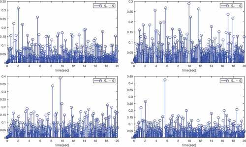The inter-event time $t_{k+1}^i-t_k^i$ and the trigger time instant $t_k^i$ of four agents are shown in Figure 12. Obviously, the Zeno behavior is excluded successfully.

Figure 3. The trajectories of $y_1$, $y_2$, $y_3$, $y_4$ and $y_0$.

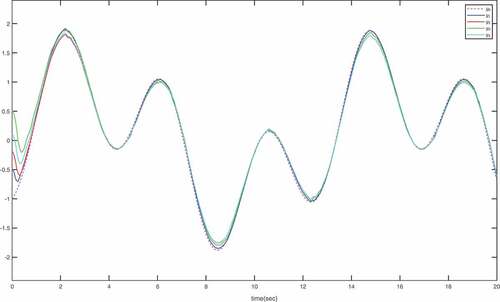
Figure 4. The curves of the tracking errors $y_i-y_0$.

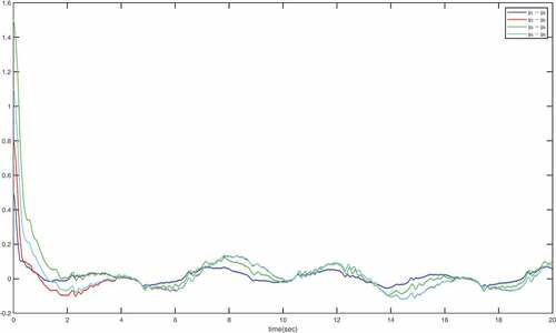
Figure 5. The trajectories of the system states ${\chi }_{i1}$ with constraints.

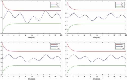
Figure 6. The trajectories of the error variables $S_{i1}$ with constraints.

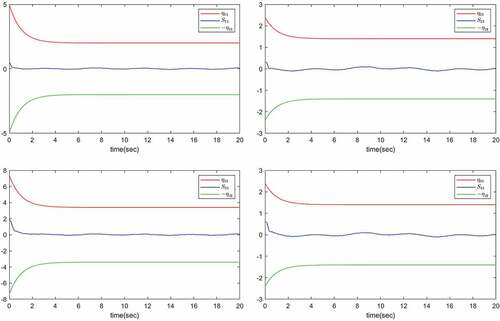
Figure 7. The trajectories of the system states ${\chi }_{i2}$ and its estimation ${\hat{\chi }}_{i1}$.

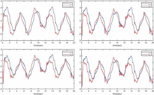
Figure 8. The curves of the controller ${\tau }_1(t)$ and its saturation input $\mathrm{s}\mathrm{a}{\mathrm{t}}_1({\tau }_1(t))$.

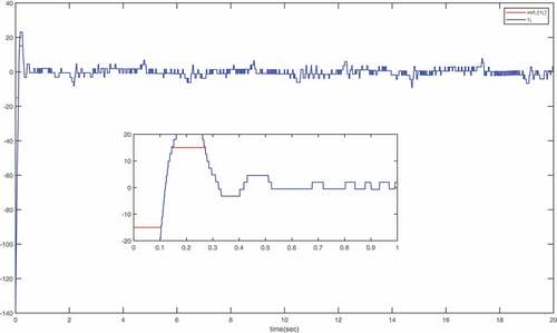
Figure 9. The curves of the controller ${\tau }_2(t)$ and its saturation input $\mathrm{s}\mathrm{a}{\mathrm{t}}_2({\tau }_2(t))$.

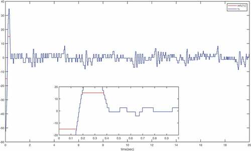
Figure 10. The curves of the controller ${\tau }_3(t)$ and its saturation input $\mathrm{s}\mathrm{a}{\mathrm{t}}_3({\tau }_3(t))$.

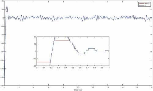
Figure 11. The curves of the controller ${\tau }_4(t)$ and its saturation input $\mathrm{s}\mathrm{a}{\mathrm{t}}_4({\tau }_4(t))$.

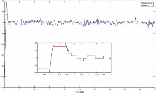
Figure 12. The inter-event time of ${\tau }_i(t)$.

To highlight the advantages of this work, a comparison with ETC scheme proposed in Yang et al. (2022) is conducted with the same parameters. Figure 13 shows the trajectories of $y_i$ and $y_0$ with ETC scheme proposed in Yang et al. (2022). The trigger numbers of the ETC scheme proposed in Yang et al. (2022) and this paper are shown in Table 1. As can be seen from Figures 3 and 13 and Table 1, even though more general cases are considered in this paper, there is no significant difference in control performance, but the number of triggers using the ETC scheme proposed in this paper is significantly less than that using the ETC scheme proposed in Yang et al. (2022)

Figure 13. The trajectories of $y_1$, $y_2$, $y_3$, $y_4$ and $y_0$ with ETC scheme proposed in Yang et al. (2022).

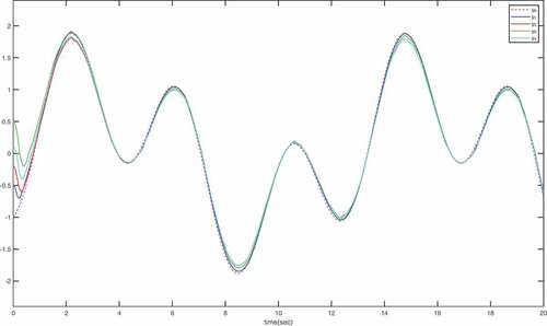
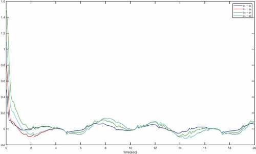
Table 1. Trigger numbers for agents.

	Agent 1	Agent 2	Agent 3	Agent 4
ETC scheme in Yang et al. (2022)	889	443	504	461
ETC scheme proposed in this paper	483	396	381	423

Remark 7. The saturation controller (7) is realized with its input defined in (87)–(89). The initial values of the constrained states should be set within the constraint boundaries. Under the proposed control scheme, all error variables converging to a neighborhood of the origin in finite time is ensured. In addition, as can be seen from Figures 8 to 11, although the required control feedback is large, the actual saturation control can still achieve satisfactory control effect.

Conclusion

An output feedback-based fuzzy adaptive finite-time ETC problem is investigated in this paper for a FOMAS with PSCs and IS in directed networks. A reduced-order state observer is designed to estimate the unmeasurable states. FLS is used to tackle the nonlinearity and the unknown parameters are estimated adaptively. A fractional-order filter is constructed to avoid repeatedly calculating the high-order derivatives of the virtual controllers. By introducing an appropriate BLF, the designed ETC scheme can ensure state constraints are not breached and the communication resources can be reduced. By analyzing the stability, it is guaranteed that finite-time tracking can be achieved with a bounded error, all signals of system are bounded and the Zeno behavior does not occur. Finally, a numerical example is given to demonstrate the effectiveness of the proposed control scheme.

Disclosure statement

No potential conflict of interest was reported by the authors.

Data availability statement

Data sharing is not applicable to this article as no new data were created or analyzed in this study.

References

- Antonio, V. T. J., G. Adrien, A. M. Manuel, P. Jean-Christophe, C. Laurent, R. Damiano, and T. Didier. 2021. Event-triggered leader-following formation control for multi-agent systems under communication faults: application to a fleet of unmanned aerial vehicles. Journal of Systems Engineering and Electronics 32 (5):1014–292. doi:10.23919/JSEE.2021.000086.
- Cajo, R., M. Guinaldo, E. Fabregas, S. Dormido, D. Plaza, R. De Keyser, and C. Ionescu. 2021. Distributed formation control for multi-agent systems using a fractional-order proportional-integral structure. IEEE Transactions on Control Systems Technology 29 (6):2738–45. doi:10.1109/TCST.2021.3053541.
- Cao, B., and X. Nie. 2021. Event-triggered adaptive neural networks control for fractional-order nonstrict-feedback nonlinear systems with unmodeled dynamics and input saturation. Neural Networks 142:288–302. doi:10.1016/j.neunet.2021.05.014.
- Chang, Y., X. Zhang, Q. Liu, and X. Chen. 2022. Sampled-data observer based event-triggered leader-follower consensus for uncertain nonlinear multi-agent systems. Neurocomputing 493:305–13. doi:10.1016/j.neucom.2022.04.071.
- Chen, B., J. Hu, Y. Zhao, and B. K. Ghosh. 2020. Leader-following consensus of linear fractional-order multi-agent systems via event-triggered control strategy. IFAC-PapersOnline 53 (2):2909–14. doi:10.1016/j.ifacol.2020.12.964.
- Chen, D., X. Liu, and W. Yu. 2020. Finite-time fuzzy adaptive consensus for heterogeneous nonlinear multi-agent systems. IEEE Transactions on Network Science and Engineering 7 (4):3057–66. doi:10.1109/TNSE.2020.3013528.
- Chen, L., Y. Wang, W. Yang, and J. Xiao. 2018. Robust consensus of fractional-order multi-agent systems with input saturation and external disturbances. Neurocomputing 303:11–19. doi:10.1016/j.neucom.2018.04.002.
- Fan, X., P. Bai, H. Li, X. Deng, and M. Lv. 2020. Adaptive fuzzy finite-time tracking control of uncertain non-affine multi-agent systems with input quantization. IEEE Access 8:187623–33. doi:10.1109/ACCESS.2020.3030282.
- Fu, J., Y. Wan, G. Wen, and T. Huang. 2019. Distributed robust global containment control of second-order multiagent systems with input saturation. IEEE Transactions on Control of Network Systems 6 (4):1426–37. doi:10.1109/TCNS.2019.2893665.
- Fu, J., G. Wen, W. Yu, T. Huang, and X. Yu. 2019. Consensus of second-order multiagent systems with both velocity and input constraints. IEEE Transactions on Industrial Electronics 66 (10):7946–55. doi:10.1109/TIE.2018.2879292.
- Fu, J., G. Wen, X. Yu, and Z. Wu. 2022. Distributed formation navigation of constrained second-order multiagent systems with collision avoidance and connectivity maintenance. IEEE Transactions on Cybernetics 52 (4):2149–62. doi:10.1109/TCYB.2020.3000264.
- Gong, P., and W. Lan. 2018. Adaptive robust tracking control for uncertain nonlinear fractional-order multi-agent systems with directed topologies. Automatica 92:92–99. doi:10.1016/j.automatica.2018.02.010.
- Gong, P., K. Wang, and W. Lan. 2019. Fully distributed robust consensus control of multi-agent systems with heterogeneous unknown fractional-order dynamics. International Journal of Systems Science 50 (10):1902–19. doi:10.1080/00207721.2019.1645913.
- Huang, X., W. Lin, and B. Yang. 2005. Global finite-time stabilization of a class of uncertain nonlinear systems. Automatica 41 (5):881–88. doi:10.1016/j.automatica.2004.11.036.
- Ling, J., X. Yuan, and L. Mo. 2019. Distributed containment control of fractional-order multi-agent systems with unknown persistent disturbances on multilayer networks. IEEE Access 8:5589–600. doi:10.1109/ACCESS.2019.2962234.
- Lin, W., S. Peng, Z. Fu, T. Chen, and Z. Gu. 2022. Consensus of fractional-order multi-agent systems via event-triggered pinning impulsive control. Neurocomputing 494:409–17. doi:10.1016/j.neucom.2022.04.099.
- Liu, J., P. Li, W. Chen, K. Qin, and L. Qi. 2019. Distributed formation control of fractional-order multi-agent systems with relative damping and nonuniform time-delays. ISA transactions 93:189–98. doi:10.1016/j.isatra.2019.03.012.
- Liu, J., P. Li, L. Qi, W. Chen, and K. Qin. 2019. Distributed formation control of double-integrator fractional-order multi-agent systems with relative damping and nonuniform time-delays. Journal of the Franklin Institute 356 (10):5122–50. doi:10.1016/j.jfranklin.2019.04.031.
- Liu, Y., H. Zhang, Z. Shi, and Z. Gao. 2022. Neural network-based finite-time bipartite containment control for fractional-order multi-agent systems. IEEE Transactions on Neural Networks and Learning Systems. doi:10.1109/TNNLS.2022.3143494.
- Li, Y., H. Wang, X. Zhao, and N. Xu. 2022. Event-triggered adaptive tracking control for uncertain fractional-order nonstrict-feedback nonlinear systems via command filtering. International Journal of Robust and Nonlinear Control 32 (14):7987–8011. doi:10.1002/rnc.6255.
- Li, Y., M. Wei, and S. Tong. 2021. Event-triggered adaptive neural control for fractional-order nonlinear systems based on finite-time scheme. IEEE Transactions on Cybernetics. doi:10.1109/TCYB.2021.3056990.
- Li, L., Y. Yu, X. Li, and L. Xie. 2022. Exponential convergence of distributed optimization for heterogeneous linear multi-agent systems over unbalanced digraphs. Automatica 141:110259. doi:10.1016/j.automatica.2022.110259.
- Ma, X., L. Yang, L. Ma, W. Dong, M. Jin, L. Zhang, F. Yang, and Y. Lin. 2022. Consensus tracking control for uncertain non-strict feedback multi-agent system under cyber attack via resilient neuroadaptive approach. International Journal of Robust and Nonlinear Control 32 (7):4251–80. doi:10.1002/rnc.6035.
- Podlubny, I. 1998. Fractional differential equations: an introduction to fractional derivatives, fractional differential equations, to methods of their solution and some of their applications. New York: Academic Press.
- Polendo, J., and C. Qian. 2005. A generalized framework for global output feedback stabilization of genuinely nonlinear systems. Proceedings of the 44th IEEE Conference on Decision and Control, Seville,Spain.
- Polycarpou, M. M., and P. A. Ioannou. 1996. A robust adaptive nonlinear control design. Automatica 32 (3):423–27. doi:10.1016/0005-1098(95)00147-6.
- Qian, C., and W. Lin. 2001. Non-Lipschitz continuous stabilizers for nonlinear systems with uncontrollable unstable linearization. Systems & Control Letters 42 (3):185–200. doi:10.1016/S0167-6911(00)00089-X.
- Qu, F., S. Tong, and Y. Li. 2018. Observer-based adaptive fuzzy output constrained control for uncertain nonlinear multi-agent systems. Information Sciences 467:446–63. doi:10.1016/j.ins.2018.08.025.
- Ren, B., S. S. Ge, K. Tee, and T. Lee. 2010. Adaptive neural control for output feedback nonlinear systems using a barrier lyapunov function. IEEE Transactions on Neural Networks 21 (8):1339–45. doi:10.1109/TNN.2010.2047115.
- Shahamatkhah, E., and M. Tabatabaei. 2020. Containment control of linear discrete-time fractional-order multi-agent systems with time-delays. Neurocomputing 385:42–47. doi:10.1016/j.neucom.2019.12.067.
- Shahvali, M., M. Naghibi-Sistani, and J. Askari. 2022. Dynamic event-triggered control for a class of nonlinear fractional-order systems. IEEE Transactions on Circuits and Systems II: Express Briefs 69 (4):2131–35. doi:10.1109/TCSII.2021.3128561.
- Shang, L., and M. Cai. 2021. Adaptive practical fast finite-time consensus protocols for high-order nonlinear multi-agent systems with full state constraints. IEEE Access 9:81554–63. doi:10.1109/ACCESS.2021.3085843.
- Sheng, D., Y. Wei, S. Cheng, and Y. Wang. 2018. Observer-based adaptive backstepping control for fractional-order systems with input saturation. ISA transactions 82:18–29. doi:10.1016/j.isatra.2017.06.021.
- Shou, Y., B. Xu, H. Lu, A. Zhang, and T. Mei. 2022. Finite-time formation control and obstacle avoidance of multi-agent system with application. International Journal of Robust and Nonlinear Control 32 (5):2883–901. doi:10.1002/rnc.5641.
- Song, S., B. Zhang, X. Song, and Z. Zhang. 2019. Neuro-fuzzy-based adaptive dynamic surface control for fractional-order nonlinear strict-feedback systems with input constraint. IEEE Transactions on Systems, Man, and Cybernetics: Systems 51 (6):3575–86. doi:10.1109/TSMC.2019.2933359.
- Viel, C., M. Kieffer, H. Piet-Lahanier, and S. Bertrand. 2022. Distributed event-triggered formation control for multi-agent systems in presence of packet losses. Automatica 141:110215. doi:10.1016/j.automatica.2022.110215.
- Wang, H., B. Chen, X. Liu, K. Liu, and C. Lin. 2013. Robust adaptive fuzzy tracking control for pure-feedback stochastic nonlinear systems with input constraints. IEEE Transactions on Cybernetics 43 (6):2093–104. doi:10.1109/TCYB.2013.2240296.
- Wang, M., B. Chen, X. Liu, and P. Shi. 2008. Adaptive fuzzy tracking control for a class of perturbed strict-feedback nonlinear time-delay systems. Fuzzy Sets and Systems 159 (8):949–67. doi:10.1016/j.fss.2007.12.022.
- Wang, C., L. Cui, M. Liang, J. Li, and Y. Wang. 2021. Adaptive neural network control for a class of fractional-order nonstrict-feedback nonlinear systems with full-state constraints and input saturation. IEEE Transactions on Neural Networks and Learning Systems. doi:10.1109/TNNLS.2021.3082984
- Wang, L., and J. Dong. 2022a. Adaptive fuzzy consensus tracking control for uncertain fractional-order multi-agent systems with event-triggered input. IEEE Transactions on Fuzzy Systems 30 (2):310–20. doi:10.1109/TFUZZ.2020.3037957.
- Wang, L., and J. Dong. 2022b. Reset event-triggered adaptive fuzzy consensus for nonlinear fractional-order multi-agent systems with actuator faults. IEEE Transactions on Cybernetics. doi:10.1109/TCYB.2022.3163528
- Wang, L., J. Dong, and C. Xi. 2020. Event-triggered adaptive consensus for fuzzy output-constrained multi-agent systems with observers. Journal of the Franklin Institute 357 (1):82–105. doi:10.1016/j.jfranklin.2019.09.033.
- Wang, C., J. Gao, M. Liang, and Y. Chai. 2020. Design of adaptive fuzzy controllers for a class of fractional-order nonlinear MIMO systems with input saturation. IEEE Access 8:104590–602. doi:10.1109/ACCESS.2020.2998681.
- Wang, C., and M. Liang. 2018. Adaptive NN tracking control for nonlinear fractional-order systems with uncertainty and input saturation. IEEE Access 6:70035–44. doi:10.1109/ACCESS.2018.2878772.
- Wang, W., L. Wang, and C. Huang. 2022. Event-triggered control for guaranteed-cost bipartite formation of multi-agent systems. IEEE Access 10:18338–51. doi:10.1109/ACCESS.2021.3086404.
- Wei, M., Y. Li, and S. Tong. 2020. Event-triggered adaptive neural control of fractional-order nonlinear systems with full-state constraints. Neurocomputing 412:320–26. doi:10.1016/j.neucom.2020.06.082.
- Wu, D., Q. An, Y. Sun, Y. Liu, and H. Su. 2021. Containment control in fractional-order multi-agent systems with intermittent sampled data over directed networks. Neurocomputing 442:209–20. doi:10.1016/j.neucom.2021.01.136.
- Yaghoubi, Z., and H. A. Talebi. 2020. Cluster consensus of fractional-order nonlinear multi-agent systems with switching topology and time-delays via impulsive control. International Journal of Systems Science 51 (10):1685–98. doi:10.1080/00207721.2020.1772404.
- Yang, Y., X. Xi, S. Miao, and J. Wu. 2022. Event-triggered output feedback containment control for a class of stochastic nonlinear multi-agent systems. Applied Mathematics and Computation 418:126817. doi:10.1016/j.amc.2021.126817.
- Yang, W., W. Yu, and W. Zheng. 2021. Fault-tolerant adaptive fuzzy tracking control for nonaffine fractional-order full-state-constrained MISO systems with actuator failures. IEEE Transactions on Cybernetics. doi:10.1109/TCYB.2020.3043039
- Ye, Y., H. Su, and Y. Sun. 2018. Event-triggered consensus tracking for fractional-order multi-agent systems with general linear models. Neurocomputing 315:292–98. doi:10.1016/j.neucom.2018.07.024.
- Zhang, H., Z. Gao, Y. Wang, and Y. Cai. 2022. Leader-following exponential consensus of fractional-order descriptor multi-agent systems with distributed event-triggered strategy. IEEE Transactions on Systems, Man, and Cybernetics: Systems 52 (6):3967–79. doi:10.1109/TSMC.2021.3082549.
- Zhao, L., X. Chen, J. Yu, and P. Shi. 2022. Output feedback-based neural adaptive finite-time containment control of non-strict feedback nonlinear multi-agent systems. IEEE Transactions on Circuits and Systems I: Regular Papers 69 (2):847–58. doi:10.1109/TCSI.2021.3124485.
- Zhou, Q., S. Zhao, H. Li, R. Lu, and C. Wu. 2019. Adaptive neural network tracking control for robotic manipulators with dead zone. IEEE Transactions on Neural Networks and Learning Systems 30 (12):3611–20. doi:10.1109/TNNLS.2018.2869375.
- Zouari, F., A. Ibeas, A. Boulkroune, J. Cao, and M. M. Arefi. 2021. Neural network controller design for fractional-order systems with input nonlinearities and asymmetric time-varying pseudo-state constraints. Chaos, Solitons, and Fractals 144:110742. doi:10.1016/j.chaos.2021.110742.