Design and Implementation of an Enterprise Credit Risk Assessment Model Based on Improved Fuzzy Neural Network

ABSTRACT

In order to improve the effect of enterprise credit risk assessment, this paper combines the improved fuzzy neural network to construct the enterprise credit risk assessment model. The various jamming patterns that can threaten the credit data transmission system include various blocking jamming and tracking jamming. Moreover, this paper analyzes the bit error performance of the credit data transmission system against various interferences, and obtains the bit error curves against various interferences through program simulation. In addition, this paper builds a variable-speed credit data transmission system based on Simulink, analyzes the key technologies in variable-speed credit data transmission, and simulates the anti-interference performance of variable-speed credit data transmission technology. The simulation study verifies that the enterprise credit risk assessment model proposed in this paper has good risk assessment effect and risk response strategy effect.

Introduction

Credit risk returns have obvious asymmetry. For unsecured loans, under normal circumstances, banks can obtain normal interest income. However, once the credit risk occurs, the losses suffered by the bank will be much larger than the interest income. Obviously, the likelihood of credit risk can be reduced if it is thoroughly reviewed (Krabec, Čižinská, and Rýdlová 2021). This asymmetry of gains and losses determines that the probability of credit risk is skewed to the left, and there will be thick tails on the left. It is because of this basic characteristic of credit risk that we cannot assume that it obeys the normal distribution, which brings great difficulties to the measurement of credit risk (Johnson, Lopez, and Sorensen 2021).

From the point of view of a single loan, since the credit risk is affected by the borrower’s operating ability, moral level, repayment willingness and financial status, its uncertainty is relatively large, and it has strong non-systematic characteristics; on the other hand, the macroeconomic All businesses will be affected by the same conditions, industry development trends, national policies, natural disasters, etc. These factors can lead to changes in the credit status of loan companies, so credit risk has certain systemic characteristics (Pechlivanidis, Ginoglou, and Barmpoutis 2021).

Since the term of most loans is relatively long, several uncertain factors will impact the loan’s repayment schedule and amount throughout its duration. Therefore, it is difficult to analyze the credit risk of commercial banks quantitatively; secondly, the impact of the financial crisis is even more challenging. The debtor is in control of modifying the unfavorable aspects of loan repayment. The lender can’t observe changes in credit risk due to information asymmetry directly (Wang et al. 2021).

Under normal circumstances, in order to obtain loans from commercial banks, borrowers are likely to provide false or incomplete information to commercial banks, so it is difficult for commercial banks as creditors to fully understand the true status of borrowers. After the commercial bank grants credit, for the borrower, driven by the maximization of its own interests, if the benefits brought by default are far greater than the risks to be undertaken, the possibility of moral hazard will increase and the borrower chooses to default. Banks not only cannot get the interest income of the credit, what is even worse is that the original credit funds cannot be repaid (Gietzmann and Wang 2020).

The credit paradox refers to the contradiction between commercial banks’ academic requirements for credit decentralization and the actual phenomenon of credit concentration. Because only through long-term business relationships can a customer’s credit status be fully understood, banks prefer to centralize loans. For the small number of old customers, this has the advantage that the bank understands the customer’s credit management situation, making it simple to grasp these situations. This approach, however, contradicts the decentralization principle of risk management. Once a default occurs, the loss will be enormous if the credit risk is too concentrated (Starko 2018).

The remainder of this paper is organized as follows: Section 2 provides the research approach’s connected work. Section 3 presents the basic theory of enterprise financial credit data transmission. Section 4 includes the enterprise credit risk assessment model. Finally, part 5 brings the study to a conclusion.

Literature Review

Literature (Bauman and Shaw 2018) proposes a Credit Metrics model to measure credit risk, which is a credit risk management model based on the VaR method, which estimates the credit risk VaR of individual securities and investment portfolios on a mark-to-market basis, fully considering Credit rating ups and downs and default events also take into account that the portfolio can play a role in diversifying risk, which is a good complement to the Basel Accord, because it recognizes the diversification effect of credit risk when assessing the market value of assets. Significance. The basic idea of this model is to calculate the default probability of certain loans based on the credit rating, and at the same time, it can calculate the probability that the above-mentioned loans will be transformed into bad debts. model to manage credit risk becomes possible. Since commercial bank loans cannot be publicly traded directly, it is difficult to obtain the market value of the loan, and the volatility of the loan value cannot be observed. The probability of change, the rate of return of the loan, etc. are used to calculate the market value and volatility of the loan for non-trading loans, and then calculate the risk reserve (Dugar and Pozharny 2021).

The neural network model consists of an input layer, several hidden intermediate layers, and an output layer. It applies neuropsychology and cognitive science research findings. The performance of the parallel distributed mode processing system created by mathematical methods is impressive. The capacity for parallel computing, fault tolerance, and self-learning. It was initially used to predict bank failure and was subsequently trained with a three-layer BP neural network. After training, any newly input company can be separated into non-bankrupt and bankrupt companies based on the weights provided by the network’s input samples (Ghosh and Xing 2021). The distribution of the model is free, which is applicable in practical problems, especially when the distribution of variables is unknown and the covariance structure is unequal, it can provide accurate classification, and financial data has the characteristics of reflecting various life characteristics of enterprises. The law of change has certain similarities with the theory of evolution. The advantage of neural network lies in its versatility, which can handle absolute variables and continuous variables well, and also has a good prediction effect in complex fields (Cordazzo and Rossi 2020). However, its work is relatively random, and in practical application, in order to obtain a better neural network structure, it needs to be continuously debugged, which consumes manpower and time, so its practical application is limited to a certain extent. Literature (Oliveira, Lustosa, and Oliveira Gonçalves 2021) compared the neural network method with the discriminant analysis method, and concluded that in the identification and prediction of credit risk, the neural network has no substantial superiority compared with the linear discriminant model, and the neural network model lacks explanation. Artificial neural networks are incapable of determining the relative weights of input variables. Due to the complexity of the neural network model, it is difficult to find a suitable model to study particular problems, which necessitates more time, manpower, and material resources and is inefficient. It is a significant innovation in research methods, but its actual effect is quite unstable. When the academic (Alexandra and Oleg 2021) uses the neural network model to discriminate and analyze 47 crisis enterprises and 47 normal enterprises, the accuracy rate of the prediction of crisis enterprises reaches 100%. The accuracy rate of multivariate discriminant analysis is only 72%: Literature (Nichita 2019) believes that the neural network model is generally more effective than the multivariate discriminant analysis and logistic regression analysis models.

Technical efficiency is an important part of studying the effectiveness of production behavior. By measuring the actual input (output) of the decision-making unit compared with its minimum (large) value, the operation status of the enterprise, the operation efficiency and the development level of the society are studied. Through the evaluation, the source and degree of ineffective production behavior can be analyzed (Pozdnyakov, Zoryana, and Tetiana 2020). In contrast, technical efficiency measures the extent to which the output of a decision-making unit is compared to the maximum work under the same factor input conditions. The greater the distance, the less efficient the technique. The conventional method for calculating technical efficiency is based on single-factor productivity. Although it is easy to calculate and analyze, it does not consider the internal relationship between factors. However, the factors’ composition will also have a more significant impact on technical efficiency (KAYGUSUZOĞLU, KARAHAN, And YILMAZ). Breaking through the single factor productivity measurement method, it will be more scientific and comprehensive to use a variety of input indicators to measure and analyze the technical efficiency of enterprises (Okoye, Offor, and Juliana 2019). According to the different methods of determining the production frontier, the technical efficiency measurement is divided into parametric methods and non-parametric methods. The parametric method requires that the form of the production function, the distribution form of the error term, the statistical characteristics of the sample, etc., be assumed in advance. The unknown parameters in the production function are estimated using the regression analysis method and the probability and statistics method. Comparison is performed to determine the respective efficiency values (Karpenko et al. 2019).

This paper combines the improved fuzzy neural network to construct the enterprise credit risk assessment model, and combines the practical data to verify the effect of the enterprise credit risk assessment model.

The Basic Theory of Enterprise Financial Credit Data Transmission

The Basic Concept of Enterprise Financial Credit Data Transmission

Enterprise financial credit data transmission is an important spread spectrum communication method. The theoretical basis of spread spectrum comes from Shannon’s information theory.

(1) $C=\mathrm{B}{log}_2\left(1+\frac{S}{N}\right)$(1)

In formula (1), the logarithm is replaced by a natural number e as the base to obtain

(2) $\frac{C}{\mathrm{B}}=1.44ln\left(1+\frac{S}{N}\right)$(2)

In the actual situation $S/N\ll 1$, we do a power series expansion of formula (1). Because the high-order term has little effect, the high-order term is omitted to get

(3) $\frac{C}{B}\approx 1.44\frac{S}{N}$(3)

When the transmission of white noise with power spectral density $n_0$ is considered in the channel of bandwidth B, and the noise power is $N=n_{0}B$, the available channel capacity is

(4) $C=\mathrm{B}{log}_2\left(1+\frac{S}{n_0\mathrm{B}}\right)$(4)

Shannon’s second theorem points out that by properly coding the information symbols, the error probability of the system can be reduced. From formula (1) and formula (3), it can be found that in addition to coding, if the bandwidth can be increased, the error probability of information transmission can also be reduced. When the bandwidth B approaches infinity, we have

(5) $\underset{\mathrm{B}\to \mathrm{\infty }}{lim}C=\underset{\mathrm{B}\to \mathrm{\infty }}{lim}\mathrm{B}\mathrm{l}\mathrm{o}{\mathrm{g}}_2\left(1+\frac{\mathrm{S}}{n_0\mathrm{B}}\right)=\underset{\mathrm{B}\to \mathrm{\infty }}{lim}\left[\frac{n_0\mathrm{B}}{\mathrm{S}}{log}_2\left(1+\frac{\mathrm{S}}{n_0\mathrm{B}}\right)\right]\frac{\mathrm{S}}{n_0}$(5)

Since there is $\underset{x\to x}{lim}\frac{1}{x}{log}_2(1+x)={log}_{2}e=1.44$, we have

(6) $\underset{B\to \mathrm{\infty }}{lim}C=1.44\frac{S}{n_0}$(6)

According to the relationship $S=R{E}_h\hspace{0.17em}$between the information energy S and the symbol rate R and the symbol energy $E_h$, $when\hspace{0.17em}B\to \mathrm{\infty }$,

(7) $\left(\frac{E_h}{n_0}\right)=\left(\frac{S}{n_0{R}_{max}}\right)=\frac{1}{1.44}=-1.6(\mathrm{d}\mathrm{B})$(7)

The frequency hopping spread spectrum processing gain is defined as

(8) $G_P=\frac{\mathrm{o}\mathrm{u}\mathrm{t}\mathrm{p}\mathrm{u}\mathrm{t}\mathrm{s}\mathrm{i}\mathrm{g}\mathrm{n}\mathrm{a}\mathrm{l}}{\mathrm{S}\mathrm{i}\mathrm{g}\mathrm{n}\mathrm{a}\mathrm{l}\mathrm{t}\mathrm{o}\mathrm{n}\mathrm{o}\mathrm{i}\mathrm{s}\mathrm{e}\mathrm{r}\mathrm{a}\mathrm{t}\mathrm{i}\mathrm{o}\mathrm{o}\mathrm{f}\mathrm{i}\mathrm{n}\mathrm{p}\mathrm{u}\mathrm{t}\mathrm{s}\mathrm{i}\mathrm{g}\mathrm{n}\mathrm{a}\mathrm{l}}=\frac{{(S/N)}_{\mathrm{o}\mathrm{u}\mathrm{t}}}{{(S/N)}_{in}}=\frac{R_s}{R_d}$(8)

The interference tolerance is defined to evaluate the enterprise financial credit data transmission system’s performance in an interference environment by $G_P$ and system loss L, as shown in formula (9)

(9) $M_j=\frac{G_p}{L{(S/N)}_{out}}$(9)

The principle of enterprise financial credit data transmission system is shown in Figure 1.

Figure 1. Schematic diagram of the transmission principle of corporate financial credit data.

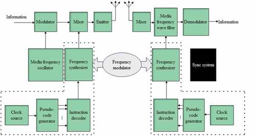
The enterprise financial credit data transmission system mainly includes: modulator, pseudo code generator, frequency synthesizer, intermediate frequency filter, demodulator, etc.

Mathematical Model of Enterprise Financial Credit Data Transmission System

If the burst information d(t) to be transmitted is a bipolar digital signal, it is expressed as

(10) $d(t)=\sum _{n=0}^{\mathrm{\infty }}{d}_n{g}_d\left(t-n{T}_d\right)$(10)

The information code is $d_n=1$ or −1, the symbol duration is $T_d,g_d(t)$ is a rectangular function, and there is $g_d(t)=\left\{\begin{array}{c}1,0\le t\le T_d\\ 0,T_d<t<0\end{array}\right.$. First, d(t) is digitally modulated, and the modulated expression is m(t), and then m(t) is subjected to frequency-hopping modulation, there are

(11) $s_1(t)=m(t)cos\left[\left(w_0+n{w}_T\right)t+{\phi }_n\right]$(11)

In Figure 2, n(t) represents noise and J(t) represents interference. Among them, $S_1(t)$ is

Figure 2. Mathematical model of enterprise financial credit data transmission system.

(12) $S_l(t)=S_1(t)+\sum _{j=1}^k{S}_j(t)+n(t)+J(t)$(12)

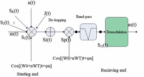
The expression after de-hop processing is

(13) $\begin{array}{rl}& S_p(t)=\left[S_1(t)+\sum _{j=1}^k{S}_j(t)+n(t)+J(t)\right]cos\left[\left(w_{r}m{w}_T\right)t+{\phi }_r\right]\\ & \hspace{0.17em}=\frac{1}{2}m(t)\left\{cos\left({\omega }_{l}t+{\phi }_J\right)+cos\left[\left({\omega }_0+w_r+2n{w}_r\right)t+{\phi }_n{\phi }_n\right]\right\}\\ & \hspace{0.17em}+\left[\sum _{j=2}^k{S}_j(t)+n(t)+J(t)\right]cos\left[\left(w_{r}m{w}_r\right)t+{\phi }_r\right]\end{array}$(13)

The signal after passing through the bandpass filter can be expressed as

(14) $S_{12}(t)=\frac{1}{2}m(t)cos\left(w_{l}t\right){\phi }_1$(14)

Main Parameters and Performance Indicators of Enterprise Financial Credit Data Transmission System

Enterprise financial credit data transmission primarily employs the following performance indicators to evaluate a frequency hopping system:

(1) Frequency hopping bandwidth

In the field of communication, the frequency band bandwidth occupied by the frequency hopping system is called the frequency hopping bandwidth, denoted as $B_{FR}$. Among them, $B_{l\cdot R}=f_{\mathrm{m}\mathrm{a}\mathrm{x}}-f_{\mathrm{m}\mathrm{i}\mathrm{n}},f_{\mathrm{m}\mathrm{a}\mathrm{x}}$ is the maximum frequency and $f_{\mathrm{m}\mathrm{i}\mathrm{n}}$ is the minimum frequency.

(2) Number of frequency hopping frequencies

The number of frequency hopping frequencies is the number of all candidate frequency hopping frequencies in the frequency hopping frequency set, which is usually denoted as N. The anti-jamming performance of the frequency hopping system is positively related to the frequency of the frequency hopping.

(3) Frequency hopping processing gain

Although there are multiple carrier frequencies in enterprise financial credit data transmission, only one carrier frequency is selected for frequency hopping modulation at a specific moment, and then IF modulation is performed. These two frequencies together determine the instantaneous spectral bandwidth $B_{I\mathrm{\prime }}$ at this time. Its ratio with the frequency hopping bandwidth (radio frequency bandwidth) $B_{lRR}$ is the frequency hopping processing gain $G_p$, which is expressed as $G_p=B_{lRR}/B_{lt}$.

(4) Frequency hopping rate

The frequency hopping rate R is referred to as the hopping rate, which is defined as the number of RF frequency hopping per second, and the unit is hops/s (hops/s). The duration of each hop is the hop period, and the hop speed and the hop period are reciprocal. If the hopping speed is $200\mathrm{h}\mathrm{o}\mathrm{p}\mathrm{s}/\mathrm{s}$, the hopping period is $5\mathrm{m}\mathrm{s}$. Usually, the hopping speed lower than $100\mathrm{h}\mathrm{o}\mathrm{p}\mathrm{s}/\mathrm{s}$ is called slow frequency hopping, $100/\sim 1000\mathrm{h}\mathrm{o}\mathrm{p}\mathrm{s}/\mathrm{s}$ is called medium speed frequency hopping, and $1000\mathrm{h}\mathrm{o}\mathrm{p}\mathrm{s}/\mathrm{s}$ above is called fast frequency hopping. In addition, it can also be defined according to the relationship between the information rate and the hopping speed.

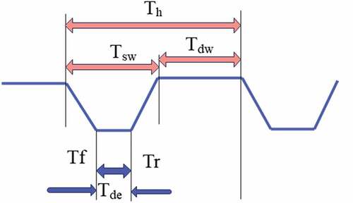
(5) Frequency hopping cycle

The frequency hopping period $T_{\mathrm{h}}$ refers to the continuous working time of each carrier frequency, that is, the time that each frequency remains unchanged in the frequency domain. It consists of frequency hopping dwell time $T_{dw}$ and channel switching time $T_{ds}$, as shown in Figure 3.

Figure 3. Remuneration relationship during the frequency hopping period.

(6) Frequency hopping sequence period

The hopping frequency varies based on the pseudo-random code, and since the frequency set is limited, the frequency sequence is eventually reused. As the sequence period, we record the maximum length of the sequence without repetition.

(7) Frequency hopping synchronization

Frequency hopping synchronization means that the sending and receiving parties use the same frequency to communicate at the same time. Usually, the frequency hopping frequency table, network number, system time information TOD, frame synchronization and bit synchronization information are required.

(8) Frequency hopping pattern

The frequency hopping varies over time, and the resulting time-frequency variation graph is known as the frequency hopping pattern. In transmitting corporate financial credit data, frequency hopping pattern design is crucial. If the enemy captures the frequency-hopping way, waveform tracking will likely interfere with it. Different frequency hopping pattern algorithms are typically employed on various occasions to improve communication security.

(9) Networking method of enterprise financial credit data transmission

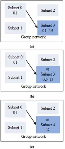
In order to enhance the anti-interference performance of enterprise financial credit data transmission, frequency hopping radio stations usually exist in the form of networking in use. According to different networking basis, it is divided into two categories: frequency packet network and code packet network. There are three networking modes: synchronous orthogonal networking, synchronous non-orthogonal networking, and asynchronous non-orthogonal networking. The call mode between network stations is shown in the figure below.

In Figure 4, Figure (a) is a network call of different subnet radio stations in the same group of networks, that is, a radio station calls all radio stations in this network or other networks. Figure (b) is the network call of the same group of network radio stations. Figure (c) shows the selective calling of radio stations in the same subnet, that is, a radio station calls another radio station in the network to realize the transmission of enterprise financial credit data.

Figure 4. Frequency hopping radio call mode.

Typical Interference Patterns in the Anti-Interference System of Enterprise Financial Credit Data Transmission

The frequency of the interference signal is fixed, and the frequency hopping of the frequency hopping signal is of no concern. The blocking interference bandwidth can be made as wide or narrow as necessary. The bandwidth is primarily divided into the following categories based on its width.

(1) Broadband Noise Blocking Interference (BBNJ)

Broadband noise interference needs to estimate the target signal bandwidth, set the interference signal according to the target bandwidth, and cover the entire target signal spectrum bandwidth as much as possible, which is also called full-band interference or blocking interference. Usually, $J_0$ represents the interference level, and the unit is $\mathrm{W}/\mathrm{H}\mathrm{z}$. Shannon channel capacity represents the maximum data transfer rate that the channel can sustain at an arbitrarily small error rate. If we want to transmit more than this rate, the reception of the information is bound to go wrong. This disturbed channel capacity is defined as

(15) $C=W_{ss}{log}_2\left(1+\frac{S}{P_1}\right)$(15)

$W_1$ is the signal bandwidth, $S$ is the average power of the signal, and $P_r=W_{ss}\left(N_0+J_0\right)$ is the total average power of the existing noise and interference.

(2) Partial Band Noise Blocking Interference (PBNJ)

Partial frequency band interference differs from broadband interference because the jammer concentrates interference power on a portion of the enterprise financial credit data transmission channel. Target channels may be adjacent or scattered. In this way, the interference is more targeted, the interference power is loaded on a part of the frequency hopping bandwidth $W_{\mathrm{w}}$, the interference power of the interfered channel is large, and the interference effect is good. Part-band interference is also very convenient to adjust the interference bandwidth. The partial frequency band interference factor $\rho$ is defined here to represent the interference bandwidth ratio.

(16) $\rho =\frac{{\mathrm{W}}_{\mathrm{J}}}{{\mathrm{W}}_{\mathrm{s}}}$(16)

Partial frequency band interference power is evenly distributed, and its unilateral power spectral density is

(17) $\frac{J}{W_J}=\frac{J}{W_{ss}}\cdot \frac{W_{sS}}{W_J}=\frac{J}{\rho W_{ss}}$(17)

When the frequency hopping signal hops into the interfered channel, the noise power spectral density has interference power in addition to the noise power, that is, $N_n=N_0+N_j\mathrm{\prime }$, otherwise there is $N_n=N_0$. For the $FH/BFSK$ system, there are

(18) $\begin{array}{rl}& {\bar{P}}_b=(1-\rho )P_b\left(\frac{E_b}{N_0}\right)+\rho \left(\frac{E_b}{N_0+N_j\mathrm{\prime }}\right)\\ & \hspace{0.17em}=\frac{1-\rho }{2}exp\left(-\frac{E_b}{2N_0}\right)+\frac{\rho }{2}exp\left(-\frac{E_b}{2\left(N_0+\frac{J}{\rho W_{ss}}\right)}\right)\end{array}$(18)

In the interference environment, there is usually $N_j\gg N_0$, so there is

(19) ${\bar{P}}_b\approx \frac{\rho }{2}exp\left(-\frac{\rho E_b}{2N_J}\right)$(19)

(3) Comb blocking jamming (CNJ)

Comb-blocking interference must first detect the minimum frequency interval between adjacent frequency points of enterprise financial credit data transmission, then adjust the interference frequency interval to the target frequency interval, and finally, concentrate the limited power on each frequency point of the frequency hopping signal. Its utilization is high and efficient, positively impacting enterprise financial credit data transmission interference.

(4) Narrow Band Interference (NBNJ)

Narrowband noise interference refers to the interference signal whose bandwidth is much smaller than the bandwidth of the target communication system. The transmission of corporate financial credit data has an inhibitory effect on narrowband interference.

Performance Analysis of Low Signal-To-Noise Ratio of Conventional Enterprise Financial Credit Data Transmission System

It is difficult to maintain phase coherence in the transmission of corporate financial credit data. Therefore, the information modulation technique adopted is usually Multi-ary Frequency Shift Keying (MFSK) or DPSK. MFSK modulation uses the mutual transformation between M carrier frequencies to transmit log2M-bit digital signals, which are generally expressed as

(20) $s_t(t)=cos\left(w_{1}t+{\phi }_1\right)$(20)

$w_i$ is M discrete values, ${\phi }_1$ is the phase constant. When the BFSK modulated signal is coherently demodulated, the bit error rate is

(21) $P_h=\frac{1}{2}erf\left(\sqrt{\frac{E_b}{2N_0}}\right)$(21)

$E_b$ is the signal energy per bit, and $N_0$ is the additive white Gaussian noise power spectral density. If non-coherent demodulation is used, the bit error rate is

(22) $P_h=\frac{1}{2}exp\left(\frac{E_h}{2N_0}\right)$(22)

Coherent demodulation needs to generate exactly the same coherent carrier, which is difficult to realize especially in phase, so non-coherent demodulation is often used in enterprise financial credit data transmission system.

(1) Analysis of anti-broadband blocking interference performance

In an environment of broadband noise interference, since the entire working frequency band is filled with additive white Gaussian noise:

(23) $P_s(M)=\frac{1}{M}exp\left(-\frac{E_s}{2\left(N_0+N_J\right)}\right)\sum _{i=2}^M\left(\begin{array}{c}M\\ i\end{array}\right)(-1{)}^{i}exp\left(-\frac{E_s(2-i)}{2\left(N_0+N_J\right)i}\right)$(23)

The bit error rate BER is

(24) $P_b=\frac{1}{2(M-1)}exp\left(-\frac{n{E}_b}{2\left(N_0+N_J\right)}\right)\sum _{i=2}^M\left(\begin{array}{c}M\\ i\end{array}\right)(-1{)}^{\prime }exp\left(-\frac{n{E}_b(2-i)}{2\left(N_0+N_J\right)i}\right)$(24)

For the FH/DPSK system, the bit error rate is the same as the conventional DPSK system in Gaussian white noise, which is

(25) $P_h=\frac{1}{2}exp\left(-\frac{E_b}{N_n}\right)=\frac{1}{2}exp\left(-\frac{1}{\frac{N_{0}R}{P}+\frac{J}{P}\frac{R}{W}}\right)$(25)

Among them, J/P is the interference signal ratio, that is, the ratio of the interference power to the signal power, and R/W is the frequency hopping processing gain.

(2) Analysis of anti-narrowband noise interference performance

The narrowband interference frequency points are randomly distributed without any regularity. When the interfering signal coincides with the target channel, a large number of bit errors will be generated. If there are K narrowband interferences in the frequency hopping bandwidth, their powers are $J_1,J_2,\cdots ,J_K$, and the single interference bandwidth is W. For a certain interference, the power spectral density is $N_{J_1}=P_{J_1}/W$. At this time, the signal-to-noise ratio of the system is $r_1=E_b/\left(N_0+N_{J_1}\right)$, then the average bit error rate of the conventional enterprise financial credit data transmission system is

(26) ${\bar{P}}_c=\frac{N-K}{N}F\left(r_0\right)+\frac{\sum _{i=1}^{K}F\left(r_i\right)}{N}$(26)

In the above formula, there is $r_0=E_h/N_0$.

(3) Analysis of anti-partial frequency band interference performance

Part-band interference is a special kind of narrowband interference. The interfering signal can be replaced with narrow-band white Gaussian noise. The interference factor $\rho =K/N,K$ is the number of selected interference frequency slots, and N is the total number of frequency hopping frequency slots. The total interference power is set to J, then the interference power spectral density is $N_J=J/\rho W_H,W_H$ is the bandwidth of a single frequency system. For the FH/BFSK system, the average bit error rate of the frequency hopping system is

(27) $\begin{array}{rl}& {\bar{P}}_c=(1-\rho )P_c\left(\frac{E_b}{N_0}\right)+\rho P_c\left(\frac{E_b}{N_0+N_J}\right)\\ & \hspace{0.17em}=\frac{(1-\rho )}{2}exp\left(-\frac{E_b}{2N_0}\right)+\frac{\rho }{2}exp\left(\frac{E_b}{2\left(N_0+J/\rho W_H\right)}\right)\end{array}$(27)

(28) ${\bar{P}}_c\approx \frac{\rho }{2}exp\left(-\frac{\rho E_h}{2N_{,}}\right)$(28)

For FH/MFSK systems, the average bit error rate is

(29) $\begin{array}{rl}& {\bar{P}}_c=(1-\rho )P_c\left(\frac{E_h}{N_0}\right)+\rho P_c\left(\frac{E_b}{N_0+N_{ȷ}}\right)\\ & \hspace{0.17em}=(1-\rho )P_c\left(\frac{P}{R{N}_0}\right)+\rho P_c\left(\frac{E_b}{\frac{R{N}_0}{P}+\frac{J}{P}\frac{R}{W}\frac{1}{\rho }}\right)\end{array}$(29)

In a disturbed environment, there is $N_J\gg N_0$, so the effect of the noise term is ignored

(30) $\begin{array}{rl}& {\bar{P}}_c=\rho P_c\left(\frac{\rho E_b}{N_{ȷ}}\right)\\ & \hspace{0.17em}=\frac{\rho }{2(M-1)}\sum _{i=2}^{M^{\prime }}\left(\begin{array}{c}M\\ i\end{array}\right)(-1{)}^{\prime }exp\left(\frac{n\rho E_b(1-i)}{N_{,j}}\right)\end{array}$(30)

Simulation condition: The frequency hopping bandwidth $50\mathrm{M}\mathrm{H}\mathrm{z}$ is set. According to the interval of each frequency slot $1\mathrm{M}\mathrm{H}\mathrm{z}$, the entire frequency hopping bandwidth is divided into N = 50 frequency slots. The $\mathrm{A}\mathrm{W}\mathrm{G}\mathrm{N}$ channel is used in the simulation, and the noise power spectral density is set to $N_0={10}^{-10}(\mathrm{W}/\mathrm{H}\mathrm{z})$. For narrowband interference, the number of interference channels is set to $\mathrm{K}$, and the interference power spectrum is −30dBW. We set the narrowband interference bandwidth $N_J$ to be the same as the frequency slot bandwidth, and the partial frequency band interference factor is $\rho =K/N$. The interference is randomly distributed in $\mathrm{K}$ frequency slots, the modulation method is MFSK, the frequency hopping speed is $1000\mathrm{h}\mathrm{o}\mathrm{p}/\mathrm{s}$, and the symbol rate is $R_s=2\mathrm{M}\mathrm{H}\mathrm{z}$.

The propagation time difference between the transmitter reaching the receiver and the transmitter reaching the jammer is denoted as $T_{\delta }$, and the time it takes the jammer to process the signal is denoted as $T_{proc}$. The generation and activation of the interference signal itself also requires a certain time, which is denoted by $T_{proc}$. The jammer processing time is $T_{pr}$, the target dwell time is $T_d$, and the effective jamming time coefficient is $\eta (0\le \eta \le 1)$. Because tracking interference requires $T_{pr}$ and location processing, there will be a certain delay $T_{n\mathrm{\prime }\mathrm{\prime }}$ when the target receives the signal containing interference.

(31) $T_{m\mathrm{\prime }j}=min\left(T_{pr}+\frac{d_2+d_3-d_1}{c},T_d\right)$(31)

Therefore, the effective interference time is $T_s=T_d-T_{n{j}^{\prime }}$, and the interference is effective only when there is $T_{nj}<T_d$. Whether the target frequency hopping signal can be interfered is affected by the probability $P_1$ that the interferer detects the target signal and the probability $P_2$ of successful release of the interference, that is, $P_J=P_1{P}_2$. The bit error rate of enterprise financial credit data transmission under interference is set to $B_J$, and the bit error rate is $B_{nj}$ when there is no interference, then B is related to the receiver signal-to-interference ratio, and $B_{nj}$ is related to the signal-to-noise ratio. Therefore, in the presence of interference, the bit error rate is $P_f{B}_f+\left(1-P_f\right)B_{nj}$, and when there is no interference, the bit error rate is $B_{nj}$, then the average bit error rate is,

(32) $\begin{array}{rl}& {\bar{P}}_c=\frac{T_s}{T_d}\left[P_{ȷ}{B}_{ȷ}+\left(1-P_{ȷ}\right)B_{nj}\right]+T_d{B}_{nj}\\ & \hspace{0.17em}=\frac{T_d-T_{nj}}{T_d}{P}_{ȷ}{B}_J+\left(1-\frac{T_d-T_{nj}}{T_d}{P}_J\right)B_{nj}\end{array}$(32)

Enterprise Credit Risk Assessment Model

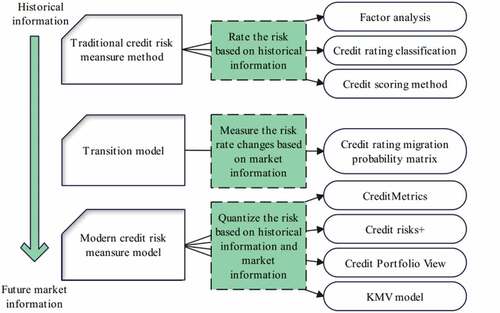
Figure 5 shows the historical evolution of credit risk assessment methods.

Figure 5. Historical evolution of credit risk assessment methods.

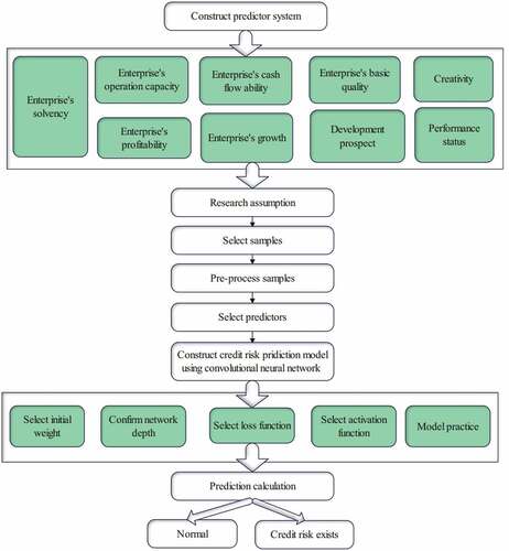
The problems existing in the current enterprise credit risk prediction index system are analyzed, and based on the previous research results, a new index system including financial and non-financial indicators is constructed. Among them, the financial indicators include five aspects: solvency, profitability, operating ability, growth ability and cash acquisition ability. The non-financial indicators include four aspects: development prospects, basic quality of enterprises, innovation capabilities, and performance of contracts. This paper presents a model for predicting credit risk based on the enhanced GoogleNet neural network. In light of the problem posed by the volume of sample data, an excessive number of input indicators will not only waste computing resources but also reduce operational efficiency. Still, it will also result in the multicollinearity of hands and diminish the training effect. Therefore, in this paper, the financial indicators are first screened twice, and then combined with the processed non-financial indicators as the model input, as shown in Figure 6.

Figure 6. The overall design of the enterprise credit risk prediction model based on the convolutional neural network method.

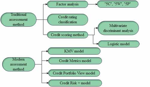
Credit risk assessment methods have undergone a transition from traditional assessment methods to modern assessment methods. However, the modern evaluation method is mainly based on quantitative analysis with the help of modern financial theory and mathematical tools, as shown in Figure 7.

Figure 7. Credit risk assessment method.

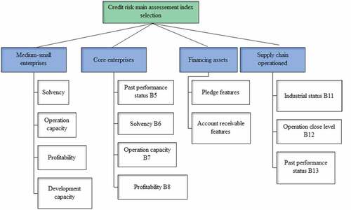
Before establishing the primary credit risk assessment indicators for small and medium-sized businesses in the economic environment of the supply chain, the primary content of the direct credit risk assessment and debt credit risk assessment indicators must be confirmed. By reading pertinent literature and gaining an in-depth understanding of supply chain finance, it is possible to conclude that the primary credit risk assessment indicators are financing enterprises, i.e., small and medium-sized businesses. As depicted in Figure 8, debt credit risk indicators mainly include core enterprises, assets under financing, and supply chain operations.

Figure 8. Selection of main evaluation indicators for credit risk.

On the basis of the above model, the effect of the enterprise credit risk assessment model proposed in this paper is verified, and the Matlab simulation is used to test the effect of statistical credit risk assessment and risk response strategy. The results are shown in Figure 9.

Figure 9. Validation of the effect of the enterprise credit risk assessment model.

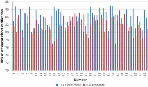
Through the above research, it is verified that the enterprise credit risk assessment model proposed in this paper has good risk assessment effect and risk response strategy effect.

Conclusion

Credit risk refers to the possibility that the borrower who has obtained the bank’s credit support will be unable or unwilling to repay the loan according to the terms of the contract, causing the bank to incur losses. Another prevalent theory holds that credit risk stems from the fluctuating value of the debt market, which is likely to result in certain bank losses. A significant drawback of Fuzzy Logic control systems is that they depend entirely on human knowledge and expertise. A fuzzy system must regularly update the rules of a control system, which is time-consuming and require massive computational resources. The former perspective focuses on whether firms default, whereas the latter examines the value changes of credit assets. Credit risk encompasses, in a broad sense, losses incurred by commercial banks due to a variety of uncertain factors. This paper combines an improved fuzzy neural network with a credit risk assessment model for enterprises. The simulation study demonstrates that the enterprise credit risk assessment model proposed in this paper has a practical risk assessment and response effects.

Disclosure Statement

No potential conflict of interest was reported by the authors.

Data Availability Statement

Data will be provided upon request

Additional information

Funding

The authors reported there is no funding associated with the work featured in this article.

References

- Alexandra, M., and P. Oleg. 2021. Methodology for brand assessment as an intangible asset in agricultural holdings. Наука о человеке: гуманитарные исследования 15 (2):196–816. doi:10.17238/issn1998-5320.2021.15.2.24.
- Bauman, M. P., and K. W. Shaw. 2018. Value relevance of customer-related intangible assets. Research in Accounting Regulation 30 (2):95–102. doi:10.1016/j.racreg.2018.09.010.
- Cordazzo, M., and P. Rossi. 2020. The influence of IFRS mandatory adoption on value relevance of intangible assets in Italy. Journal of Applied Accounting Research 21 (3):415–36. doi:10.1108/JAAR-05-2018-0069.
- Dugar, A., and J. Pozharny. 2021. Equity investing in the age of intangibles. Financial Analysts Journal 77 (2):21–42. doi:10.1080/0015198X.2021.1874726.
- Ghosh, A. A., and C. Xing. 2021. Goodwill impairment and audit effort. Accounting Horizons 35 (4):83–103. doi:10.2308/HORIZONS-19-055.
- Gietzmann, M., and Y. Wang. 2020. Goodwill valuations certified by independent experts: Bigger and cleaner impairments? Journal of Business Finance & Accounting 47 (1–2):27–51. doi:10.1111/jbfa.12411.
- Johnson, P. M., T. J. Lopez, and T. L. Sorensen. 2021. Did SFAS 141/142 improve the market’s understanding of net assets, goodwill, or other intangible assets? Review of Quantitative Finance and Accounting 56 (3):891–915. doi:10.1007/s11156-020-00912-x.
- Karpenko, L., P. Pashko, P. Voronzhak, H. Kalach, and M. Nazarov. 2019. Formation of the system of fair business practice of the company under conditions of corporate responsibility. Academy of Strategic Management Journal 18 (2):1–8.
- Krabec, T., R. Čižinská, and B. Rýdlová. 2021. Deconstruction of inherent goodwill generated in owner-managed companies in the Czech republic. International Advances in Economic Research 27 (3):253–55. doi:10.1007/s11294-021-09834-3.
- Nichita, M. E. 2019. Intangible assets–insights from a literature review. Journal of Accounting and Management Information Systems 18 (2):224–61. doi:10.24818/jamis.2019.02004.
- Okoye, P. V. C., N. Offor, and M. I. Juliana. 2019. Effect of intangible assets on performance of quoted companies in Nigeria. International Journal of Innovative Finance and Economics Research 7 (3):58–66.
- Oliveira, K. V., P. R. B. Lustosa, and A. Oliveira Gonçalves. 2021. Goodwill from the appreciative inquiry (AI) perspective: Innovation transforming intangible capital. Revista Contemporânea de Contabilidade 18 (47):03–17. doi:10.5007/2175-8069.2021.e75538.
- Pechlivanidis, E., D. Ginoglou, and P. Barmpoutis. 2021. Can intangible assets predict future performance? A deep learning approach. International Journal of Accounting and Information Management 30 (1):61–72. doi:10.1108/IJAIM-06-2021-0124.
- Pozdnyakov, Y. V., S. Zoryana, and G. Tetiana. 2020. Price-forming factors choice grounding at intangible assets with negative depreciation independent valuation/appraising. Independent Journal of Management & Production 11 (6):2112–39. doi:10.14807/ijmp.v11i6.1170.
- Starko, I. 2018. Normal regulation of the recognition and evaluation of the goodwill. Review of Accounting Studies 17 (4):749–80.
- Wang, Y., T. Li, D. Wang, and K. Liu. 2021. Has damage from goodwill impairment grown in China? Analysis and response. China Journal of Accounting Studies 9 (2):168–94. doi:10.1080/21697213.2021.1992936.