Image polar radius distribution for seed orientation adjustment

ABSTRACT

Seed orientation is an important factor in high-speed automatic seeders used for sowing crops such as garlic cloves and corn kernels. However, obtaining accurate seed orientation angles can be challenging due to high-frequency noise points and false top features in seed images, which can negatively impact the orientation effect. In this paper, we introduce a directional adjustment method based on the polar radius distribution map to address this issue. Our method involves two main steps. Firstly, we use the morphological opening operation to process speckles and some seed apex parts and use the region marker to obtain the original polar radius distribution curve signal. Secondly, we use the wavelet packet transform to analyze the original polar radius distribution curve signal, which yields a direction rotation angle after analysis and calculation and enables the determination of seed orientation. Our experimental results show that our method can better identify the germination location at the top of the seed, and the calculated rotation angle is more conducive to seed direction adjustment than the rotation angle directly determined by the maximum polar radius in the polar radius vector. This is due to the advantage of higher frequency resolution of wavelet packet analysis, which enables us to obtain a polar radius distribution curve signal with low noise, better smoothness, and more realistic reflection of the edge characteristics of the seed contour boundary. The proposed method provides an effective solution for accurately adjusting the orientation of garlic cloves and corn kernels and potentially other crops that require automation technology. Our key finding is that using the polar radius distribution map and wavelet packet transform can yield better results in seed orientation adjustment, by removing high-frequency noise points and false top features and improving the accuracy of seed rotation angle calculation.

Introduction

Large-scale farming of crops such as garlic, sunflower, and maize requires accurate seed orientation to promote better rooting and germination (Joshi et al. 2018; Zhou et al. 2016). Determining seed orientation is called orientation adjustment, typically done using visual technology (Chen et al. 2022; Liu and Paulsen 2000; Wang et al. 2008). However, before the orientation adjustment process, image preprocessing steps must be taken to ensure accurate edge detection (Zhang 2020) and noise reduction. The canny operator is commonly used for edge detection due to its edge positioning accuracy and anti-noise performance. However, the detected edges may be discontinuous and may not completely describe the contour characteristics of the seed shape. Additionally, the top features of the seed skin shape may cover up the real position information of the seed germination position, leading to incorrect orientation adjustment results.

To address these issues, various methods have been proposed for representing the seed contour, including scale descriptor and angle descriptor (Ballard 1981; Pospisil, Pasupathy, and Bair 2018; Ulrich, Steger, and Baumgartner 2003; Zhang 2021). The angle descriptor has local characteristics but cannot capture all the contour change information, leading to the loss of local contour information at the seed germination location. On the other hand, the scale descriptor captures all the contour change information in the longitudinal orientation and reflects the overall contour characteristics.

In this paper, we propose a method for seed orientation adjustment based on the scale descriptor. Our proposed method involves the use of morphological technology to obtain a high-quality point set of seed boundary contour, multi-scale wavelet packet analysis to obtain a low-frequency signal of the polar radius distribution curve with low noise and better smoothness, and an algorithm flow of rotation angle to determine seed orientation (Hasim, Herdiyeni, and Douady 2016; Wang, Kim, and Chen 2009).

The motivation behind our research is to improve the efficiency and effectiveness of large-scale farming by providing a more accurate and reliable method for seed orientation adjustment. The proposed orientation adjustment method first uses connected region marking (Qiao 2004). There are many such methods (AbuBaker 2007; Suzuki, Horiba, and Sugie 2003). In this paper, morphological region marking (Motameni 2007; Zhang et al. 2019) and fast boundary calculation based on run-length coding (Li et al. 2018; Quek 2000) are used to obtain the contour point set and the centroid of the garlic clove or corn kernel boundary. Then, the polar radius variation curve corresponding to the polar radius scale descriptor is used to explore garlic clove and corn kernel orientation adjustment. Finally, the rotation parameters for orientation adjustment are obtained by combining multiscale wavelet packet analysis and rotation angle calculation (Hemmati, Orfali, and Gadala 2016).

The method of the seed direction adjustment introduced in this paper uses morphological technology to solve the problem that the top part of the seed skin conceals the real position information of the seed germination part, avoid the occurrence of discontinuous edges, and obtain a high-quality point set of seed boundary contour, which reflects a complete edge contour; By using multi-scale wavelet packet analysis technology, the low-frequency signal of the polar radius distribution curve with low noise and better smoothness is obtained, which effectively removes the high-frequency noise points at the edge of the seed image, and finally captures the real position of seed germination; The algorithm flow of rotation angle which is easy to realize in engineering is given (Demertzis, Iliadis, and Anezakis 2017; Li et al. 2019; Wu and Du 1996). To intuitively express the orientation adjustment effect, the cutting regions of each garlic clove are obtained according to the set of boundary outline points of each clove in the image. In each region, the filtering method based on geometric features is used to obtain the subset image of each garlic clove in the image, and then orientation adjustment is performed by using the method proposed in this paper. We also apply this method to corn kernel orientation adjustment and achieve the same effect.

The rest of this article is organized as follows. In Section 2, we describe the basic theoretical analysis used in our research. In Section 3, we present the general flow of seed orientation adjustment. Section 4 presents the experimentations. The discussion containing the significance and potential applications of our research is presented in Section 5. Finally, in Section 6, we conclude the paper and suggest future research directions.

Basic Theoretical Analysis

Polar Radius Distribution Shearing Zone Distribution

As shown in Figure 2(a), the variable polar radius $\overrightarrow{OA}$ traverses all the boundary points clockwise along the boundary contour to obtain the polar radius feature vector of the boundary contour. Figure 2(b) shows the expansion diagram corresponding to the polar radius vector for the step $\mathrm{\Delta }\mathrm{\varnothing }$. The expansion diagram can be regarded as a polar radius expansion curve signal, which reflects the overall boundary contour characteristics. The coordinates of the geometric center O are given by Eq. (1)(1) $\left\{\begin{array}{c}\bar{x}=\frac{{\sum }_{\mathrm{i}}^{\mathrm{N}}{\mathrm{x}}_{\mathrm{i}}}{\mathrm{N}}\\ \bar{y}=\frac{{\sum }_{\mathrm{i}}^{\mathrm{N}}{\mathrm{y}}_{\mathrm{i}}}{\mathrm{N}}\end{array}\right.$(1) ,

(1) $\left\{\begin{array}{c}\bar{x}=\frac{{\sum }_{\mathrm{i}}^{\mathrm{N}}{\mathrm{x}}_{\mathrm{i}}}{\mathrm{N}}\\ \bar{y}=\frac{{\sum }_{\mathrm{i}}^{\mathrm{N}}{\mathrm{y}}_{\mathrm{i}}}{\mathrm{N}}\end{array}\right.$(1)

where $x_i$ and $y_i$ denote the row coordinates and column coordinates of a point $i$, respectively, in the boundary contour point set and $N$ denotes the total number of boundary points. Figure 1 presents the expansion principle corresponding to the polar radius feature vector.

Figure 1. Expansion principle corresponding to the polar radius feature vector.

Figure 2. Shearing process diagram.

As shown in Figure 2(a), when object A is cut, part of object B is also cut.

The R in Figure 2 is a rectangle, which is determined as a shear area. The size of the rectangle is determined by the set of boundary contour points, and the specific operation is given by Eq. (2)(2) $\left\{\begin{array}{c}{x}_0=x_{min}-\mathrm{\Delta }x,\cdot \cdot \cdot \cdot x_0>0\\ y_0=y_{min}-\mathrm{\Delta }y,\cdot \cdot \cdot \cdot y_0>0\\ x_w=x_{max}-x_{min}+\mathrm{\Delta }{x}_w\\ y_h=y_{max}-y_{min}+\mathrm{\Delta }{y}_h\end{array}\right.$(2) . Here, $\left(x_0,y_0\right)$ denotes the coordinates of the upper left corner of rectangle R, and $x_w$ $y_h$ denote the width and height of rectangle R, respectively. In addition, $x_{min}$ and $y_{min}$ are the minimum x coordinate and minimum Y coordinate in the boundary contour point set, respectively, and $x_{max}$ $y_{max}$ denote the maximum x coordinate and maximum Y coordinate, respectively, in the boundary contour point set. Finally, $\mathrm{\Delta }x$ and $\mathrm{\Delta }y$ denote the shear margin of the upper left corner of rectangle R, $\mathrm{\Delta }{x}_w$ and $\mathrm{\Delta }{y}_h$ are the shear margins of rectangle R in the width and height orientations, respectively. The function of the shear margin value is to stay within the boundary of the shear zone when the object rotates during the process of displaying orientation adjustment.

(2) $\left\{\begin{array}{c}{x}_0=x_{min}-\mathrm{\Delta }x,\cdot \cdot \cdot \cdot x_0>0\\ y_0=y_{min}-\mathrm{\Delta }y,\cdot \cdot \cdot \cdot y_0>0\\ x_w=x_{max}-x_{min}+\mathrm{\Delta }{x}_w\\ y_h=y_{max}-y_{min}+\mathrm{\Delta }{y}_h\end{array}\right.$(2)

Figure 2(b) shows the shearing results. Because objects A and B are adjacent to each other, part of the area of object B, i.e., area C, is also cut when separating object A. Therefore, when the orientation of object A is adjusted, it is necessary to remove area C first.

Basic Theory of Multiscale Wavelet Packet Analysis

The wavelet packet transform (Liu et al. 2020) is a more precise analysis method than the wavelet transforms. The former can divide the high- and low-frequency signal parts in a binary manner, which overcomes the low-resolution disadvantage of the wavelet transform for high-frequency signals. Its basic idea is to decompose the wavelet subspace in multiresolution analysis, and the signal is processed through a series of low-pass and high-pass filter banks to obtain decomposition coefficients and then accomplish reconstruction according to the decomposition coefficients to obtain low-frequency signals with low noise and better smoothness, which can truly reflect the seed edge features. Given the orthogonal scaling function and the wavelet function, the two-scale equation is shown in Eq. (3)(3) $\left\{\begin{array}{c}{\varphi }_0(t)=\sqrt{2}{\sum }_{k\in z}{h}_{0k}\varphi (2t-k)\\ {\varphi }_1(t)=\sqrt{2}{\sum }_{k\in z}{h}_{1k}\varphi (2t-k)\end{array}\right.$(3) ,

(3) $\left\{\begin{array}{c}{\varphi }_0(t)=\sqrt{2}{\sum }_{k\in z}{h}_{0k}\varphi (2t-k)\\ {\varphi }_1(t)=\sqrt{2}{\sum }_{k\in z}{h}_{1k}\varphi (2t-k)\end{array}\right.$(3)

where $h_{0k}$ and $h_{1k}$ are low-pass and high-pass filter banks of multiresolution analysis, respectively. Eq. (4)(4) $\left\{\begin{array}{c}{w}_{2n}(t)=\sqrt{2}{\sum }_{k\in z}{h}_{0k}{w}_n(2t-k)\\ w_{2n+1}(t)=\sqrt{2}{\sum }_{k\in z}{h}_{1k}{w}_n(2t-k)\end{array}\right.$(4) is the general form of the two-scale Eq. (3)(3) $\left\{\begin{array}{c}{\varphi }_0(t)=\sqrt{2}{\sum }_{k\in z}{h}_{0k}\varphi (2t-k)\\ {\varphi }_1(t)=\sqrt{2}{\sum }_{k\in z}{h}_{1k}\varphi (2t-k)\end{array}\right.$(3) .

(4) $\left\{\begin{array}{c}{w}_{2n}(t)=\sqrt{2}{\sum }_{k\in z}{h}_{0k}{w}_n(2t-k)\\ w_{2n+1}(t)=\sqrt{2}{\sum }_{k\in z}{h}_{1k}{w}_n(2t-k)\end{array}\right.$(4)

where $n=0$. Eq. (4)(4) $\left\{\begin{array}{c}{w}_{2n}(t)=\sqrt{2}{\sum }_{k\in z}{h}_{0k}{w}_n(2t-k)\\ w_{2n+1}(t)=\sqrt{2}{\sum }_{k\in z}{h}_{1k}{w}_n(2t-k)\end{array}\right.$(4) can be written as

(5) $\left\{\begin{array}{c}{w}_0(t)=\varphi (t)\\ w_1(t)=\psi (t)\end{array}\right.$(5)

A Set ${\left\{w_n(t)\right\}}_{n\in N}$ is defined as a wavelet packet. It is a set of functions containing the scale function $w_0(t)$ and wavelet-generating function $w_1(t)$. The wavelet packet space is composed of a scaling translation system of $w_n$, as shown in Eq. (6)(6) $W_j^n=span{\left\{2^{-j/2}{w}_n(2^{-j}t-k)\right\}}_{k\in z}$(6) , where $n\in N$ and $(j,k)\in Z^2$.

(6) $W_j^n=span{\left\{2^{-j/2}{w}_n(2^{-j}t-k)\right\}}_{k\in z}$(6)

The wavelet packet operation includes wavelet packet decomposition and reconstruction. The wavelet packet decomposition coefficients can be evaluated as

(7) $\left\{\begin{array}{c}{d}_k^{j+1,2n}=\sum _l{h}_{0(2l-k)}{d}_l^{j,n}\\ d_k^{j+1,2n+1}=\sum _l{h}_{1(2l-k)}{d}_l^{j,n}\end{array}\right.$(7)

where $d_k^{j+1,2n}$ and $d_k^{j+1,2n+1}$ are wavelet packet decomposition coefficients and $h_{0(2l-k)}$ $h_{1(2l-k)}$ are the low-pass and high-pass filter banks, respectively, of the wavelet packet decomposition. Here, $\left\{d_l^{j,n}\right\}$ is given by Eq. (8)(8) $\begin{array}{r}{d}_l^{j,n}=\sum _k[h_{0(l-2k)}{d}_k^{j+1,2n}+h_{1(l-2k)}{d}_k^{j+1,2n+1}]\\ =\sum _k[g_{0(l-2k)}{d}_k^{j+1,2n}]+\sum _k[g_{1(l-2k)}{d}_k^{j+1,2n+1}]\end{array}$(8) , where $g_{0(l-2k)}$ and $g_{1(l-2k)}$ are the low-pass and high-pass filter banks, respectively, of the wavelet packet reconstruction. This calculation process is called wavelet packet reconstruction.

(8) $\begin{array}{r}{d}_l^{j,n}=\sum _k[h_{0(l-2k)}{d}_k^{j+1,2n}+h_{1(l-2k)}{d}_k^{j+1,2n+1}]\\ =\sum _k[g_{0(l-2k)}{d}_k^{j+1,2n}]+\sum _k[g_{1(l-2k)}{d}_k^{j+1,2n+1}]\end{array}$(8)

Orientation Angle Adjustment Analysis

The index number of the maximum polar radius is found in the low-frequency signal obtained after wavelet packet decomposition and reconstruction. According to the index number, the corresponding coordinate of the boundary point is found in the boundary point set of the seed contour, which is the location of the seed apex. The distribution quadrant of the seed apex position in the coordinate system is shown in Figure 3.

Figure 3. Location distribution diagram for the seed apex, (a) first-quadrant location, (b) second-quadrant location, (c) third-quadrant location, and (d) fourth-quadrant location.

Point B is the apex position, point O is the geometric center of the shape of the contour, $\overrightarrow{OA}$ is the vertical orientation, and the angle $\mathrm{\angle }OAB$ enclosed by polar radius $\overrightarrow{OB}$ and vertical orientation is the orientation adjustment angle. The process of calculating the orientation adjustment angle is as follows. First, the coordinate differences $\mathrm{\Delta }x$ $\mathrm{\Delta }y$ between point B and point O are given by Eq. (9)(9) $\left\{\begin{array}{c}\mathrm{\Delta }x=abs(B_x-O_x)\\ \mathrm{\Delta }y=abs(B_y-O_y)\end{array}\right.$(9) :

(9) $\left\{\begin{array}{c}\mathrm{\Delta }x=abs(B_x-O_x)\\ \mathrm{\Delta }y=abs(B_y-O_y)\end{array}\right.$(9)

Second, the quadrant position of point B is determined, and the corresponding orientation adjustment angle is given by the flowchart shown in Figure 4.

Figure 4. Flowchart for calculating orientation adjustment angle θ .

Finally, according to the obtained orientation adjustment angle $\theta$, the nearest-neighbor interpolation method (Ahmad, Naz, and Razzak 2021; Jiang, Han, and Fan 1997; Laine and Fan 1993) is used to show the orientation adjustment results.

The General Flow of Seed Orientation Adjustment

Figure 5 shows the process of orientation adjustment.

Figure 5. Flow of the orientation adjustment process.

First, we use Wiener filtering operations to filter a seed image collected by an industrial camera, and then, according to the gray histogram distribution of the filtered seed image, the threshold value is determined manually, and the binary image is given. The speckles in the binary image are filtered by only one morphological open operation filtering, which involves first decomposing the binary image and then expanding it. The shape of the seed boundary contour is not significantly affected, so only the seed objective is included in the binary image.

Second, to show the orientation adjustment effect, the coordinate set of boundary pixels in the seed-connected region is obtained by the region labeling method, and then the rectangular region of a single seed is determined for shear separation.

Third, in the process of shearing and separating the designated seed object, because the seed object adjacent to the designated seed object is inevitably sheared, there are also some connected areas of the adjacent seed object in the separated image in addition to the connected area of the seed object. To solve this problem, we use a filtering method based on the characteristic parameters to filter the adjacent region and obtain a subset image that contains only the connected region of a single seed object.

Finally, the region marker is used to obtain the boundary pixel coordinate set of the seed in the shearing region, and the polar radius vector is formed to generate the signal of the polar radius distribution curve reflecting the overall characteristics of the seed contour shape. The signal is analyzed to find the real apex position of the seed, calculate the rotation angle of orientation adjustment, and output the adjustment image.

During orientation adjustment, the location and size of the shear region affect individual seed target extraction, thus affecting the generation of the polar radius feature vector of individual seed targets, which is not conducive to analyzing polar radius curve signals corresponding to the polar radius feature vector. In addition, the high-frequency noise at the seed edge affects the correct extraction of the seed apex position. Therefore, based on basic theoretical analysis, in this paper, a principle for generating a polar radius curve signal and a method for determining the shear region is proposed.

Using the theory of multiscale wavelet packet decomposition and reconstruction, the low-frequency signal of the polar radius curve reflecting the overall seed contour characteristics is extracted, and high-frequency noise is eliminated. The angle calculation method for orientation adjustment proposed in this paper is used for the orientation adjustment of a seed target.

Experiments

Experimental Settings and Preprocessing

Figure 6 shows the original experimental image with a size of 449 × 341 pixels. The image was captured by an MV-VS 200FM industrial camera under a diffuse reflective dome red light source. To verify the robustness of the algorithm, the garlic cloves in Figure 6 that are in various positions, directions, sizes, and numbers are picked. Although there are two garlic cloves in Figure 6 and 6(c), the two garlic cloves in Figure 6(a) greatly differ in shape and size. However, both positional poses are almost similar. On the other hand, the shape and size of the two garlic cloves in Figure 6(c) differ only slightly.

Figure 6. Flowchart to calculate orientation adjustment angle: (a) garlic cloves with different shapes and sizes, (b) single garlic cloves, and (c) garlic cloves with similar shapes and sizes.

To verify the stability, robustness, and generalizability of the proposed method, we implement these three types of garlic clove images as experimental objects. There are many garlic cloves in one image and some of them maybe are adhesive and overlapping, which makes image recognition difficult. Therefore, in the actual operation, the separation mechanical device and vibration mechanical device are used to obtain the separated garlic cloves with different poses in the platform area under the camera.

According to the orientation adjustment flow shown in Figure 5, the binary images are attained and shown in Figure 7.

Figure 7. Binary images: (a) large difference in shape and size, (b) single garlic clove, (c) similar shape and size.

To extract more informative images of garlic cloves, the irrelevant parts of the images are blackened by using a threshold score of 0.2, which is decided by trial and error to reach more refined binary images of garlic cloves. Even though the 0.2 threshold provides operable images, we also used filtering to remove small spots in binary images shown in Figure 8. The filtering implemented is called morphological opening to better separate garlic cloves.

Figure 8. The results of morphological openings: (a) opening result for Figure 7(a), (b) opening result for Figure 7(b), and (c) opening result for Figure 7(c).

The morphological opening operator is a disk-shaped structuring element with a radius of 3 pixels, which is decided not to harm the images of garlic cloves presented in Figure 8 which is then compared with Figure 7. The derived Figure 8(a) shows all spots get filtered. Although the spots in Figure 8(c) are not filtered, they are completely separated from the main garlic clove objects, so they do not pose any issues in the process. The three binary images in Figure 8 show that some false tops of the garlic clove are separated or filtered, which is beneficial to make an orientational adjustment. The existence of these false tops is mainly caused by the skin of garlic cloves, which is not the place where garlic cloves germinate. When the process of adjusting the direction of garlic cloves is in use, a point is selected as close to the germination position as possible to conduct the computation of a rotation angle. Ideally, this point should be located at a position where germination will occur. The symbol ﹡in Figure 8 denotes the geometric centroid position of the garlic cloves.

While Figure 9(a) shows the polar radius curve of the garlic clove in Figures 7(b), 9(b) shows the polar radius curve of the garlic clove in Figure 8(b). Figure 9 shows that the conduct of the open morphological filtering operation will result in some slight changes in the boundary contour of the seed. However, this has little effect on the polar radius distribution.

Figure 9. Polar radius distribution curve: (a) polar radius curve for the garlic clove in Figure 7(b), (b) polar radius curve for the garlic clove in Figure 8(b).

After running the morphological opening, the binary image of the garlic clove is further filtered based on characteristic parameters.

The characteristic parameter in this paper is the area whose threshold was picked at 450 since we try to observe how much will be removed. The coordinate set of boundary points in the connected areas of the garlic cloves is given by the method called region labeling. The shear rectangle region is determined by Eq. (2)(2) $\left\{\begin{array}{c}{x}_0=x_{min}-\mathrm{\Delta }x,\cdot \cdot \cdot \cdot x_0>0\\ y_0=y_{min}-\mathrm{\Delta }y,\cdot \cdot \cdot \cdot y_0>0\\ x_w=x_{max}-x_{min}+\mathrm{\Delta }{x}_w\\ y_h=y_{max}-y_{min}+\mathrm{\Delta }{y}_h\end{array}\right.$(2) , and the shear results are shown in Figure 10. When the garlic cloves in Figure 8(a) are sheared and separated, the shearing results include the part of the area of the adjacent garlic clove except that the image of the single-garlic clove not being affected by other garlic cloves. To obtain the orientation adjustment effect of a single garlic clove, it is necessary to filter the redundant area again by using the filtering method based on the characteristic parameters. The area threshold is picked at 6,400 since this image only contains a single garlic clove. Thus, the reduction of the characteristic parameter, that is, area, is merely dependent upon the specialty of the binary image in use. The filtering result is shown in Figure 11, in which the symbol * represents the centroid of each garlic clove after running shearing and filtering.

Figure 10. Shearing results: (a) shearing result 1 for Figure 8(a), (b) shearing result 2 for Figure 8(a), (c) shearing result for Figure 8(b), (d) shearing result 1 for Figure 8(c), (e) shearing result 2 for Figure 8(c) .

Figure 11. Filtering results based on feature parameters.

The key work in the image processing of garlic cloves as comprehensively described above is to identify morphological areas, that is, the identification of connected areas with closed contours. On the one hand, the characteristic parameter of each connected area can be obtained, and the reasonable threshold value for the characteristic parameter can be selected to effectively remove the unwanted connected areas, such as the top part of the garlic skin separated after running the operation of morphological opening. On the other hand, the set of boundary points of the garlic clove connected area can represent the complete edge contour of the garlic clove. Because of the large number of boundary points, it is impossible to list them one by one, but they can be represented by the distribution curve of a polar radius. The data of the aforementioned process are shown in Table 1.

Table 1. Data related to the pretreated garlic cloves.

	Garlic cloves with different shapes and sizes		Single garlic clove	Garlic cloves of similar shape and size
	Garlic clove 1	Garlic clove 2	Garlic clove 3	Garlic clove 4	Garlic clove 5
Centroid before shearing	(178.87,147.08)	(356.54,203.63)	(254.25,132.36)	(114.19,132.30)	(312.90,251.55)
$(x_{min},y_{min})$	(1,5)	(277,98)	(126,41)	(26,24)	(157,103)
$(x_{max},y_{max})$	(286,261)	(446,330)	(376,257)	(236,283)	(415,338)
Centroid after shearing	(178.68,147.04)	(95.54,121.63)	(144.25,107.36)	(104.19,124.30)	(171.90,164.55)

The shear region is jointly determined by the data in Table 1 and Eq. (2)(2) $\left\{\begin{array}{c}{x}_0=x_{min}-\mathrm{\Delta }x,\cdot \cdot \cdot \cdot x_0>0\\ y_0=y_{min}-\mathrm{\Delta }y,\cdot \cdot \cdot \cdot y_0>0\\ x_w=x_{max}-x_{min}+\mathrm{\Delta }{x}_w\\ y_h=y_{max}-y_{min}+\mathrm{\Delta }{y}_h\end{array}\right.$(2) . The margin value of the upper left corner for the shear region is picked 15, and the margin values of the height and width orientations are selected 45 since an empirical approach is adopted based on data at hand. The change in the centroid value of garlic cloves before and after shearing separation is due to the change in shape, which results in an alteration in the coordinate value of each point in the boundary point set of the garlic clove.

Figs. 12–14 show the original polar radius curves of the garlic cloves in Figure 11. The set of garlic clove boundary points are required to plot these curves that are given by preprocessing the image shown in Figure 11 generated by a method called region labeling, and the centroid coordinates are needed to calculate the polar radius that are the values of the centroid coordinate after shearing presented in Table 1.

Figure 12. Low-frequency signals given by wavelet packet multiscale decomposition and reconstruction for the garlic clove image in Figure 7(a): (a) Original polar radius curve for garlic clove 1. (b) Layer 1 reconstruction signal for garlic clove 1. (c) Layer 2 reconstruction signal for garlic clove 1. (d) Layer 3 reconstruction signal for garlic clove 1. (e) Layer 4 reconstruction signal for garlic clove 1. (f) Layer 5 reconstruction signal for garlic clove 1. (g) Original polar radius curve for garlic clove 2. (h) Layer 4 reconstruction signal for garlic clove 2.

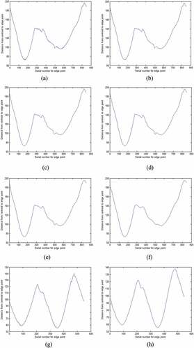
Figure 13. Layer 4 low-frequency signal given by wavelet packet multiscale decomposition and reconstruction for the single-garlic clove image in Figure 7(b). (a) Original polar radius curve for garlic clove 3. (b) Layer 4 reconstruction signal for garlic clove 3.

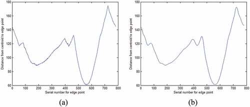
Figure 14. Layer 4 low-frequency signal given by wavelet packet multiscale decomposition and reconstruction for the garlic clove image in Figure 7(c). (a) Original polar radius curve for garlic clove 4. (b) Layer 4 reconstruction signal for garlic clove 4. (c) Original polar radius curve for garlic clove 5. (d) Layer 4 reconstruction signal for garlic clove 5.

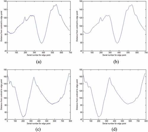
The theory of wavelet packet decomposition and reconstruction suggests that Figs. 12(b-f) shows the five-layer low-frequency signals of the polar radius curve of garlic clove 1 in Figure 7(a). Since the available space is limited to present the outcomes, Figures 12(h), 13(b), and Figs. 14(b, d) shows only the low-frequency signal of the fourth layer for the other garlic cloves in Figure 7.

Implementation

The original curve corresponding to the polar radius vector clearly shows that the curve is a nonstationary signal and is susceptible to the influence of high-frequency noise points on the edge of the garlic clove. The peaks of the curves in Figs. 12(a, g) may be noise points. Therefore, accurate recognition of the apex position of the garlic clove is difficult, and further processing of the distribution curve signal of the original polar radius is required. Because wavelet packet analysis has the advantage of high-frequency resolution and can remove noise well, we use a wavelet packet called coif5 to decompose and reconstruct the distribution curve signal of the original polar radius. So, the corresponding low-frequency signals of five layers are given. The low-frequency signals of the five layers shown in Figure 12 present the processing results for garlic clove 1 in the garlic clove image shown in Figure 7(a). However, some noise remains in the low-frequency signals of the first and second layers. Alternatively, the low-frequency signals of the third and fourth layers well reflect the cusp characteristic of the garlic clove, but the fifth layer signal is distorted.

The peak of the curve in Figure 13(a) may be noise points too. The low-frequency signal of the fourth layer in Figure 13(b) well reflects the cusp characteristic of the garlic clove.

The cusp feature of the apex position of the garlic clove in Figure 14(a) is not obvious, and the curve signal of the polar radius distribution shows that there exist some noise points. In addition, the peak of the curve in Figure 14(c) may be noise points. The fourth layer signal after conducting wavelet packet analysis is shown in Figs. 14(b, d) has lower noise, better smoothness, and more truly reflects the edge characteristics of the seed contour。

To sum up, this paper uses the fourth-level signal as the reference to obtain the cusp position coordinates to conduct scale descriptor analysis.

Discussion

The relevant data obtained from the Layer 4 signal are shown in Table 2. The parameters in Table 2 are the parameters presented in Eq. 9(9) $\left\{\begin{array}{c}\mathrm{\Delta }x=abs(B_x-O_x)\\ \mathrm{\Delta }y=abs(B_y-O_y)\end{array}\right.$(9) and Figure 5, respectively, and the index number shows the element’s serial number in the boundary point set of the garlic clove.

Table 2. Relevant data are given before and after processing the polar radius signal with a wavelet packet.

	Original polar radius curve					Polar radius signal processed by the wavelet packet
	Garlic clove 1	Garlic clove 2	Garlic clove 3	Garlic clove 4	Garlic clove 5	Garlic clove 1	Garlic clove 2	Garlic clove 3	Garlic clove 4	Garlic clove 5
Index number	824	477	724	545	784	827	479	724	543	790
$(B_x,B_y)$	(2,236)	(35,248)	(22,232)	(80,275)	(16,231)	(2,233)	(34,246)	(22,232)	(240,217)	(16,225)
$\mathrm{\Delta }x$	176.68	60.54	122.25	24.19	155.9	176.68	61.54	122.25	112.81	53.10
$\mathrm{\Delta }y$	88.96	126.37	124.64	150.70	66.45	85.96	124.37	124.64	115.7	148.55
$\theta$	243.28	205.60	224.45	189.12	66.91	244.06	206.33	224.45	225.72	19.67

Table 2 depicts that according to the polar radius signals of the garlic cloves before and after wavelet packet processing, the index numbers corresponding to the two maximum polar radii are given. Besides, the serial numbers of the garlic cloves change, except for the serial number of a single garlic clove presented in Figure 7(b)), which also leads to a change in the adjustment angle $\theta$of the orientation Moreover, the noise points at the edge of the image of the garlic clove do adversely affect the calculation of rotation angle. Therefore, removing these noise points is conducive to direction adjustment. So, the visual representation of the data in Table leads to Figures 15–20, which shows the adjustment effect of the clove orientation.

Figure 15. Orientation adjustment results for the garlic cloves in Figure 7(a) (polar radius curve without wavelet packet processing). (a) the maximum polar radius of garlic clove 1. (b) Maximum polar radius of garlic clove 2. (c) Orientation adjustment for garlic clove 1. (d) Orientation adjustment for garlic clove 2.

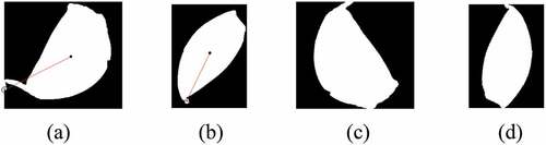
Figure 16. Orientation adjustment results for the garlic cloves in Figure 7(a) (polar radius curve processed by the wavelet packet). (a) the maximum polar radius of garlic clove 1. (b) Maximum polar radius of garlic clove 2. (c) Orientation adjustment for garlic clove 1. (d) Orientation adjustment for garlic clove 2.

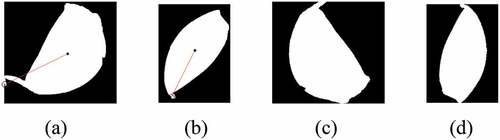
Figure 17. Orientation adjustment result for garlic clove 3 in Figure 7(b) (polar radius curve without wavelet packet processing). (a) the maximum polar radius of garlic clove 3. (b) Orientation adjustment for garlic clove 3.

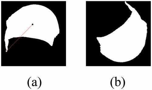
Figure 18. Orientation adjustment result for garlic clove 3 in Figure 7(b) (polar radius curve processed by the wavelet packet). (a) the maximum polar radius of garlic clove 3. (b) Orientation adjustment for garlic clove 3.

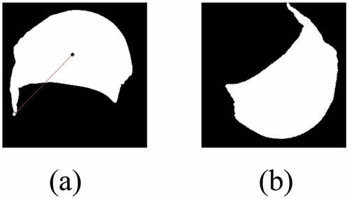
Figure 19. Orientation adjustment results for the garlic cloves in Figure 7(c) (polar radius curve without wavelet packet processing). (a) the maximum polar radius of garlic clove 4. (b) Maximum polar radius of garlic clove 5. (c) Orientation adjustment result for garlic clove 4. (d) Orientation adjustment result for garlic clove 5.

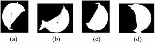
Figure 20. Orientation adjustment results for the garlic cloves in Figure 7(c) (polar radius curve processed by the wavelet packet). (a) the maximum polar radius of garlic clove 4. (b) Maximum polar radius of garlic clove 5. (c) Orientation adjustment result for garlic clove 4. (d) Orientation adjustment result for garlic clove 5.

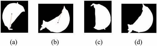
Figs. 15(c, d) show the orientation adjustment effects of non-wavelet packet processing for the polar radius signal. The red lines in Figs. 15(a, b) are the polar radii of garlic cloves 1 and 2, respectively.

On the contrary, Figure 16 shows the orientation adjustment effects of wavelet packet processing for the polar radius signal. When compared with that in Figure 15, the result of the orientation adjustment shown in Figure 16 exhibits a slight change.

Figure 17(b) shows the effects of the orientation adjustment of non-wavelet packet processing for the polar radius signal. The red line in Figure 17(a) represents the polar radius of garlic clove 3.

In contrast, Figure 18 shows the effects of the orientation adjustment of wavelet packet processing for the polar radius signal. When compared with that in Figure 17, the result of the orientation adjustment in Figure 18 shows no change, which indicates that the image of the original garlic clove contains less noise at the apex position but a higher image quality.

Figs. 19(c, d) shows the effects of the orientation adjustment of non-wavelet packet processing for the polar radius signal. The red lines in Figs. 19(a, b) denote the polar radii of garlic clove 4 and 5, respectively.

When compared with that in Figure 19, the adjustment result of the clove orientation shown in Figure 20 is significantly improved due to wavelet packet analysis processing. To further verify the stability, robustness, and generalizability of the suggested approach, shearing, and orientation adjustment of the corn kernel image shown in Figure 21 are performed.

Figure 21. Original image.

After running the Wiener filtering on the original image, the same threshold, 0.2, is used to obtain the binary image, as shown in Figure 22. Figure 23 shows the results of the orientation adjustment, which meets the direction conditions when sowing corn seeds.

Figure 22. Binary image.

Figure 23. Results of orientation adjustment for corn kernels.

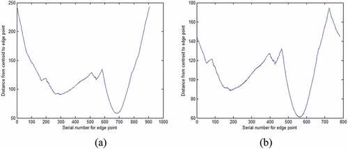
The original polar radius curves of only the fourth and seventh corn kernels are presented in Figures 24 and 26 due to space limitations. These curves are decomposed and reconstructed by the wavelet packet called coif5 to obtain the low-frequency signal of the fourth layer that is shown in Figures 25 and 27. Figures 24 and 26 suggest that there is no prominent cusp feature at the top of the original polar radius curve. After this curve is decomposed and reconstructed by running the wavelet packet, the cusp feature of the corresponding top position of the fourth-layer low-frequency signal is improved significantly, which is beneficial in recognizing the top of the corn kernel. Table 3 shows the related data in the orientation adjustment process of the corn kernel.

Figure 24. Original polar radius curve for the 4th corn kernel.

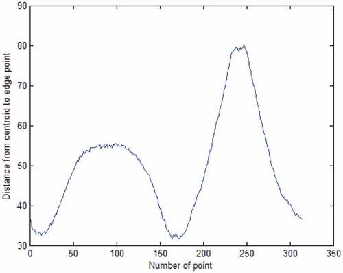
Figure 25. Layer 4 reconstruction signal for the 4th corn kernel.

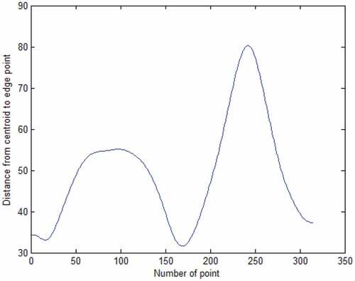
Figure 26. Original polar radius curve for the 7th corn kernel. Fig. 27. Layer 4 reconstruction signal for the 7th corn kernel.

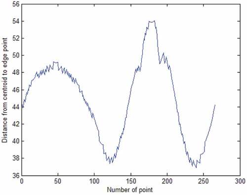
Figure 27. Layer 4 reconstruction signal for the 7th corn kernel.

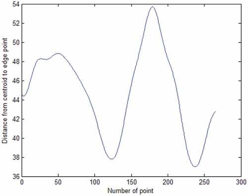
Table 3. Relevant data of corn kernel polar radius signals processed by the wavelet packet.

	Polar radius signal processed by the wavelet packet
	Corn kernel 1	Corn kernel 2	Corn kernel 3	Corn kernel 4	Corn kernel 5	Corn kernel 6	Corn kernel 7
Centroid after shearing	(68.93,67.47)	(61.18,53.37)	(49.30,96.31)	(51.89,68.41)	(66.18,64.93)	(67.67,62.91)	(55.44,65.14)
$\left(B_x,B_y\right)$	(138,108)	(111,48)	(26,17)	(23,142)	(34,17)	(16,86)	(55,119)
$x$	69.07	49.82	23.30	28.89	32.18	51.67	0.44
$y$	40.53	5.37	79.31	73.59	47.93	23.09	53.86
$\theta$(degrees)	120.4	83.84	343.63	201.44	326.12	245.92	180.47

Table 3 depicts the rotation angle, $\theta$, of the orientation adjustment. All the orientation adjustment processes in the research are realized by rotating the angle, $\theta$, in the counterclockwise direction around the centroid. The orientation adjustment results of the corn kernel presented in Figure 23 are given by rotating the corresponding value $\theta$ in Table 3 in the counterclockwise direction.

Conclusion

In this paper, we present a method for seed orientation adjustment based on the polar radius distribution map. This research is motivated by the increasing use of high-speed automatic seeders in modern agriculture, which require accurate seed orientation to ensure efficient and effective planting.

Based on the vector of the crop seed boundary point set, the overall seed boundary contour characteristics with the scale descriptor polar radius are described in this paper. The polar radius curve, i.e., polar radius signal, is generated. The morphological technique introduced in this paper ensures that the boundary point set can describe the complete edge contour of the seed. The wavelet packet’s decomposition and reconstruction theory is introduced into the signal analysis, which effectively removes the influence of noise points, improves the cusp feature of the seed top position, and yields a better seed orientation adjustment effect. In this paper, garlic cloves and corn kernels are taken as research objects, and a good orientation adjustment effect is achieved.

We use morphological techniques to ensure that the boundary point set can describe the complete edge contour of the seed. Our method describes the overall seed boundary contour characteristics using the scale descriptor polar radius, which generates a polar radius curve or signal. Additionally, we introduce the theory of decomposition and reconstruction of the wavelet packet into the signal analysis, which effectively removes the influence of noise points and improves the cusp feature of the seed top position.

In our experiments, we applied our method to garlic cloves and corn kernels as research objects and achieved a good orientation adjustment effect. The experimental results demonstrate that our method is stable and robust and has reference significance for certain crop seeds that need to be planted on a large scale with automation technology. The experimental results show that our method has certain stability and robustness, and reference significance for certain crop seeds that need to be planted on a large scale with automation technology.

Our research contributes to a more accurate and reliable method for seed orientation adjustment. Our method yields better results than the traditional method of determining the seed rotation angle directly by the maximum polar radius in the polar radius vector.

In conclusion, our research provides a practical and effective solution for accurate seed orientation adjustment in modern agriculture. The method we propose is not only limited to garlic cloves and corn kernels but also applies to other crops requiring automation technology. We believe that our method can significantly improve the efficiency and productivity of modern agriculture, and we hope that our work can inspire further research in this field.

Disclosure statement

No potential conflict of interest was reported by the author(s).

Data Availability statement

Data will be provided on request ([email protected]).

Additional information

Funding

This study was supported by the National Natural Science Foundation of China (No. 61673252) and Major Project of Basic Science (Natural Science) Research among Colleges and Universities in Jiangsu Province (No. 22kja460001).

References

- AbuBaker, A. 2007. One scan connected the component labeling technique. In 2007 IEEE International Conference on Signal Processing and Communications (ICSPC), 1283–958. doi:10.1109/icspc.2007.4728561.
- Ahmad, R., S. Naz, and I. Razzak. 2021. Efficient skew detection and correction in scanned document images through clustering of probabilistic Hough transforms. Pattern Recognition Letters 152:93–99. doi:10.1016/j.patrec.2021.09.014.
- Ballard, D. H. 1981. Generalizing the Hough transform to detect arbitrary shapes. Pattern Recognition 13 (2):111–22. doi:10.1016/0031-3203(81)90009-1.
- Chen, M., X. Yan, M. Cheng, P. Zhao, Y. Wang, R. Zhang, X. Wang, J. Wang, and M. Chen. 2022. Preparation, characterization and application of poly (lactic acid)/corn starch/eucalyptus leaf essential oil microencapsulated active bilayer degradable film. International Journal of Biological Macromolecules 195:264–73. doi:10.1016/j.ijbiomac.2021.12.023.
- Demertzis, K., L. Iliadis, and V.D. Anezakis. 2017. A deep spiking machine-hearing system for the case of invasive fish species. In 2017 IEEE International Conference on INnovations in Intelligent SysTems and Applications (INISTA), 23–28. doi:10.1109/INISTA.2017.8001126.
- Hasim, A., Y. Herdiyeni, and S. Douady. 2016. Leaf shape recognition using centroid contour distance. IOP Conference Series 31 (012002):1–8. doi:10.1088/1755-1315/31/1/012002.
- Hemmati, F., W. Orfali, and M. S. Gadala. 2016. Roller bearing acoustic signature extraction by wavelet packet transform, applications in fault detection and size estimation. Applied Acoustics 104:101–18. doi:10.1016/j.apacoust.2015.11.003.
- Jiang, H. -F., C. -C. Han, and K. -C. Fan. 1997. A fast approach to the detection and correction of skew documents. Pattern Recognition Letters 18 (7):675–86. doi:10.1016/s0167-8655(97)00032-9.
- Joshi, A., S. Kaur, K. Dharamvir, H. Nayyar, and G. Verma. 2018. Multi-walled carbon nanotubes applied through seed-priming influence early germination, root hair, growth and yield of bread wheat (Triticum aestivum L.). Journal of the Science of Food and Agriculture 98 (8):3148–60. doi:10.1002/jsfa.8818.
- Laine, A., and J. Fan. 1993. Texture classification by wavelet packet signatures. IEEE Transactions on Pattern Analysis and Machine Intelligence 15 (11):1186–91. doi:10.1109/34.244679.
- Li, S., J. Shang, Z. Duan, and J. Huang. 2018. Fast detection method of quick response code based on run‐length coding. IET Image Processing 12 (4):546–51. doi:10.1049/iet-ipr.2017.0677.
- Li, X., X. Zhang, P. Zhang, and G. Zhu. 2019. Fault data detection of traffic detector based on wavelet packet in the residual subspace associated with PCA. Applied Sciences 9 (17):3491. doi:10.3390/app9173491.
- Liu, J., and M. Paulsen. 2000. Corn whiteness measurement and classification using machine vision. Transactions of the ASAE 43 (3):757–63. doi:10.13031/2013.2759.
- Liu, W., X. Yang, S. Jinxing, and C. Duan. 2020. An integrated fault identification approach for rolling bearings based on dual-tree complex wavelet packet transform and generalized composite multiscale amplitude-aware permutation entropy. Shock and Vibration 2020:1–18. doi:10.1155/2020/8851310.
- Motameni, H. 2007. Labeling method in steganography. International Journal of Computer and Information Engineering 1 (6):1600–05. doi:10.105281/zenodo.1062790.
- Pospisil, D. A., A. Pasupathy, and W. Bair. 2018. ’artiphysiology’reveals V4-like shape tuning in a deep network trained for image classification. Elife 7:e38242. doi:10.7554/eLife.38242.
- Qiao, J. 2004. Mobile fruit grading robot (part 1) development of a robotic system for grading sweet peppers. Journal of the Japanese Society of Agricultural Machinery 66 (2):113–22. doi:10.11357/jsam1937.66.2_113.
- Quek, F. K. 2000. An algorithm for the rapid computation of boundaries of run-length encoded regions. Pattern Recognition 33 (10):1637–49. doi:10.1016/s0031-3203(98)00118-6.
- Suzuki, K., I. Horiba, and N. Sugie. 2003. Linear-time connected-component labeling based on sequential local operations. Computer Vision and Image Understanding 89 (1):1–23. doi:10.1016/s1077-3142(02)00030-9.
- Ulrich, M., C. Steger, and A. Baumgartner. 2003. Real-time object recognition using a modified generalized Hough transform. Pattern Recognition 36 (11):2557–70. doi:10.1016/S0031-3203(03)00169-9.
- Wang, S., H. Kim, and H. Chen. 2009. Contour tracking using centroid distance signature and dynamic programming method. In 2009 International Joint Conference on Computational Sciences and Optimization, IEEE, 274–78. doi:10.1109/CSO.2009.201.
- Wang, W., J. Li, F. Huang, and H. Feng. 2008. Design and implementation of log-gabor filter in fingerprint image enhancement. Pattern Recognition Letters 29 (3):301–08. doi:10.1016/j.patrec.2007.10.004.
- Wu, Y., and R. Du. 1996. Feature extraction and assessment using wavelet packets for monitoring machining processes. Mechanical Systems and Signal Processing 10 (1):29–53. doi:10.1006/mssp.1996.0003.
- Zhang, B. 2020. A multispectral image edge detection algorithm based on improved canny operator. In International Conference in Communications, Signal Processing, and Systems(CSPS, 1298–307. doi:10.1007/978-981-13-9409-6_155.
- Zhang, S. -X. 2021. Adaptive boundary proposal network for arbitrary shape text detection. In Proceedings of the IEEE/CVF International Conference on Computer Vision (ICCV), 1285–1294. doi:10.1109/ICCV48922.2021.00134.
- Zhang, W., Z. Mi, Y. Zheng, Q. Gao, and W. Li. 2019. Road marking segmentation based on siamese attention module and maximum stable external region. IEEE Access 7:143710–20. doi:10.1109/access.2019.29944993.
- Zhou, R., R. Zhou, X. Zhang, J. Zhuang, S. Yang, K. Bazaka, and K. Ostrikov. 2016. Effects of atmospheric-pressure N2, He, Air, and O2 microplasmas on mung bean seed germination and seedling growth. Scientific Reports 6 (1):1–11. doi:10.1038/srep32603.