Towards Autonomous Driving Model Resistant to Adversarial Attack

ABSTRACT

Connected and Autonomous Vehicles (CAVs) offer improved efficiency and convenience through innovative embedded devices. However, the development of these technologies has often neglected security measures, leading to vulnerabilities that can be exploited by hackers. Conceding that a CAV system is compromised, it can result in unsafe driving conditions and pose a threat to human safety. Prioritizing both security measures and functional enhancements on development of CAVs is essential to ensure their safety and reliability and enhance consumer trust in the technology. CAVs use artificial intelligence to control their driving behavior, which can be easily influenced by small changes in the model that can significantly impact and potentially mislead the system. To address this issue, this study proposed a defense mechanism that uses an autoencoder and a compressive memory module to store normal image features and prevent unexpected generalization on adversarial inputs. The proposed solution was studied against Hijacking, Vanishing, Fabrication, and Mislabeling attacks using FGSM and AdvGAN against the Nvidia Dave-2 driving model, and was found to be effective, with success rates of $93.8\mathrm{\%}$ and $91.2\mathrm{\%}$ in a Whitebox setup, and $74.1\mathrm{\%}$ and $64.4\mathrm{\%}$ in a Blackbox setup for FGSM and AdvGAN, respectively. That improves the results by $24.7\mathrm{\%}$ in Whitebox setup $21.5\mathrm{\%}$ in Blackbox setup.

Introduction

Connected and autonomous vehicles (CAVs) are a type of transportation that use a combination of connected and automated technology to either support or fully replace human involvement in the driving process. These vehicles are equipped with a range of advanced technologies, such as sensors, machine learning algorithms, onboard and remote processing capabilities, Global Positioning System (GPS), and telecommunications networks, which allow them to function autonomously. (Elliott, Keen, and Miao 2019)

According to a market research report, the autonomous car market is expected to experience significant growth in the coming years, with a compound annual growth rate of $22.75\mathrm{\%}$ predicted between 2021 and 2027. This growth is expected to take the value of the market from USD 22.22 billion in 2021 to USD 75.95 billion in 2027 (MordorIntelligence 2021). The increasing prevalence of level 2 and level 3 autonomous vehicles, which are capable of greater levels of autonomy, is expected to drive this market growth by 2030.

While the use of autonomous vehicles has the potential to bring many benefits, such as improved safety, reduced congestion, and lower fuel consumption, the safety of these systems is a major concern. One approach to improving the control of autonomous vehicles is the use of end-to-end learning (e2e), which involves using deep learning algorithms to transform perceptual inputs, such as images, into control decisions such as steering angles (Bojarski et al. 2016). Research has shown that this approach (Bojarski et al. 2016) is effective, particularly when learning to emulate human drivers.

However, it is known that deep learning systems relying upon patterns within data can fall prey to adversarial interference. Adversarial interference is defined as a deliberate manipulation of input data resulting in erroneous or malicious outcomes from the machine learning model. In the context of deep learning, adversarial examples can be devised to deceive the model, leading to misclassification of images for instance. This vulnerability stems from the sensitivity of deep learning systems to slight alterations in input data that can significantly impact the output of the model. Furthermore, the intricacies of deep learning models, with their non-linear complexity, present challenges in detecting and mitigating adversarial interference. Hence, deep learning systems are at risk to various attack types,

However, it is important to note that deep learning systems can be vulnerable to adversarial interference in their inputs, which can potentially compromise the safety of the autonomous driving system.

In addition to the safety concerns related to the use of autonomous vehicles, there are also a number of other challenges that need to be addressed in order to fully realize the potential of these systems. These challenges include regulatory and legal issues, the need for infrastructure and communication systems to support autonomous driving, and the need to address privacy and security concerns related to the collection and use of data by autonomous vehicles. Despite these challenges, it is clear that connected and autonomous vehicles have the potential to transform the transportation industry and bring significant benefits to society.

There have been various strategies proposed for defending against adversarial examples, which are inputs specifically designed to cause a machine learning model to make mistakes. These strategies can be broadly classified into two categories. The first category involves improving the machine learning model or training set through techniques such as modifying the network architecture, altering the model’s loss function, and increasing the size of the training dataset. These approaches aim to increase the model’s resistance to adversarial attacks (Papernot et al. 2016; Tramèr et al. 2017 by making it more robust to slight variations in the input data. Particularly, modifying the network architecture can involve adding more layers or neurons to the model, which can increase its capacity to learn and better handle adversarial examples. Modifying the loss function can involve adding regularization terms to the optimization objective, which can help the model generalize better to unseen data. Increasing the size of the training dataset can also help the model generalize better and become more resistant to adversarial attacks, as it has more examples to learn from. However, one of the key limitations of this approach is that the model must be retrained in order to incorporate these changes, which means that it cannot defend against unknown threats.

The second category of defensive strategies involves adjusting adversarial inputs to make them more similar to clean inputs, rather than modifying the model or training process. This can involve using techniques such as input preprocessing, which involves applying transformations to the input data before it is fed into the model. In particular, adding noise (Goodfellow, Shlens, and Szegedy 2014a) to the input data or applying image processing techniques such as blurring can help make adversarial examples less effective. Another approach is to use adversarial training, which involves generating adversarial examples during the training process and adding them to the training dataset. This helps the model learn to be more resistant to adversarial attacks. One of the advantages of this approach is that the model does not need to be retrained (Guo et al. 2017), as it has already learned to handle adversarial examples during training. However, it is important to note that these defensive strategies may not be effective against all types of adversarial examples (Song et al. 2017; Zhou, Liang, and Chen 2020), and further research is needed to improve their effectiveness.

One potential reason for the effectiveness of Generative Adversarial Networks (GAN) in reconstructing adversarial samples is the strong generalization abilities of neural networks. There are several factors that may contribute to this, including overfitting, the structural similarities between adversarial and normal samples, and the lack of a clear boundary between the two. The inclusion of unlabeled adversarial samples in the training data can further exacerbate this issue, as autoencoders are designed to minimize reconstruction error for all samples, including adversarial ones.

In this study, we assess the performance of various defense approaches that are commonly used, such as auto-encoder (Wang et al. 2014), block switching (Pang et al. 2020), adversarial training (Goodfellow, Shlens, and Szegedy 2014b), defensive distillation (Papernot et al. 2016), and feature squeezing (Liu, Daniel Wang, and Song 2015). However, the diversity of generative models can result in reconstructed images that differ from the original inputs, and the high representation capacity of Convolutional Neural Networks (CNN) allows for the reconstruction of adversarial perturbations. These factors can make the aforementioned defense mechanisms complex and prone to failure. To address these limitations and defend against unknown threats, we do not train the model using adversarial examples. Instead, we propose a system that cleans adversarial inputs and makes them more similar to the original inputs captured by the CAV’s camera. We also introduce a memory module to store the original data features. The requirement for enhanced representation learning models for sequential and structured data has inspired the development of memory. Autoencoders, as a type of learning technique, aim to learn compact representations of the input data. However, conventional autoencoders lack the ability to store information about the input data, thus rendering the task of learning representations for sequential and structured data challenging.

The major contribution of this paper is addressed as follows:

• We proposed a defense mechanism to the adversarial attack in an autonomous driving model, which purifies the adversarial samples into clean samples.

• In this study we use a memory module to improve the model’s ability to capture and maintain the features of the input examples.

• Our proposed method achieves a reasonable performance compared to the most common defense approaches.

Background and Related Work

Pomerleau’s pioneering work on the Autonomous Land Vehicle in a Neural Network (ALVINN) technology in 1989 (Pomerleau 1988) was a major milestone in the development of autonomous vehicles. Pomerleau’s research demonstrated that a fully trained neural network could be used to successfully guide a car on public highways, using sensor data and machine learning algorithms to make driving decisions. This work laid the foundation for the development of later autonomous vehicle technologies, such as DAVE-2 (Bojarski et al. 2016). DAVE-2 is a further development of the ALVINN technology that was inspired by Pomerleau’s work. One of the key differences between ALVINN and DAVE-2 is the increased availability of data and computing power that has become available over the past 25 years. These advancements have allowed for the development of more complex and sophisticated autonomous vehicle systems that can handle a wider range of driving scenarios. DAVE-2 is distinguished by its ability to use these advances in technology to perform autonomous driving tasks more effectively and reliably than earlier systems.

Adversarial attacks are a type of malicious attack on machine learning models that involve introducing small, imperceptible perturbations to the input data in order to mislead the model into making incorrect predictions. These perturbations are known as adversarial examples, and they can cause the model to classify the original input as a different class than it would normally predict (Goodfellow, Shlens, and Szegedy 2014a). Adversarial attacks can be classified as Whitebox (Huang et al. 2017) or Blackbox (Papernot et al. 2017) attacks based on the knowledge required to execute the attack.

Whitebox attacks require extensive knowledge of the target model, including the training data, neural network architecture, parameters, hyperparameters, and the ability to obtain the model’s gradients and prediction outputs. This type of attack involves a direct, unrestricted access to the model, allowing the attacker to fully understand its internal workings and design the most effective adversarial examples. In contrast, Blackbox attacks only involve querying the model with arbitrary input data and receiving a predicted result. The attacker does not have access to the model’s internal details, and can only observe the model’s input-output behavior. This makes Blackbox attacks more challenging, as the attacker must find a way to generate adversarial examples without full knowledge of the model’s workings.

One way that attackers can perform Blackbox attacks is by creating a substitute model based on the input and output data of the target model. The substitute model is designed to mimic the behavior of the target model as closely as possible, using the same type of machine learning algorithms and input features. The attacker can then execute Whitebox attacks on the substitute model in order to generate adversarial examples that are effective against the target model. This approach is known as transferability of adversarial examples, and it refers to the ability to use adversarial examples created for the substitute model to successfully attack the target Blackbox model.

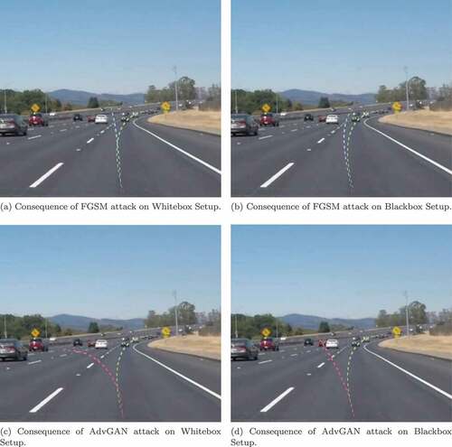
In this study, we investigate different type of adversarial attacks. In Hijacking Adversarial Attack the attacker modifies the actual trajectory of the model. This type of attack involves manipulating the model’s output in a way that causes it to take a different action than it would normally take. For example, in case of an autonomous vehicle, an adversarial attack could be used to cause the vehicle to turn left instead of right, or to brake unexpectedly Figure 1. Hijacking Adversarial Attacks can be particularly dangerous, as they can have significant consequences for the safety of the model’s users and the surrounding environment. Therefore, it is important for machine learning models to be robust against this type of attack in order to ensure their safety and reliability.

Figure 1. Change of trajectory in after FGSM and AdvGAN attack in both whitebox and blackbox setup. The green line shows the actual trajectory.

Vanishing Adversarial Attacks are designed to cause an object detection system to fail to recognize an object in an image or video by adding small perturbations to the object that are undetectable to the human eye. These perturbations can take the form of noise or other distortions added to the image or video, and they can be generated using algorithms that search for the minimum amount of perturbation needed to cause the object detection system to fail.

Fabrication Adversarial Attacks are similar to Vanishing attacks, but they involve adding fake objects to an image or video rather than modifying existing objects. These fake objects can be designed to be indistinguishable from real objects to the human eye, but they can cause object detection systems to fail by confusing them with the real objects within image or video.

Mislabeling Adversarial Attacks are also similar to Vanishing attacks, but they involve changing the label or classification of an object in an image or video rather than causing the object to disappear entirely. For example, an attacker could use a Mislabeling attack to cause a object detection system to label a car as a bicycle, or a pedestrian as a tree.

Adversarial training is a widely-used method for increasing the robustness of machine learning models. However, it can be resource-intensive due to the need to generate a large number of adversarial examples, and it may not be effective at protecting against unknown adversarial threats. Researchers have found that various types of image manipulation, such as adding noise (Shixiang and Rigazio 2014), scaling (Guo et al. 2017), JPEG compression (Buckman et al. 2018), and more, can undermine the effectiveness of adversarial attacks. One commonly used technique to counter adversarial perturbations is image denoising, such as using an Auto-Encoder to clean up adversarial examples before feeding them into a target model (Jalal et al. 2017). Another approach is to use generative networks like Defense-GAN (Samangouei, Kabkab, and Chellappa 2018) or PixelDefend (Song et al. 2017) to transform adversarial samples into clean ones. However, this requires solving an optimization problem, which can be computationally difficult and vulnerable to advanced attack methods. Defense-GAN uses latent encoding to generate clean samples directly, but this can result in a loss of model accuracy as the classifier is unable to effectively identify the purified samples. Our solution relies on a memory module containing clean features to help the model reconstruct clean images using the input image as a prior. We use the discriminator of generative network to assist with this process and adjust the weight of the reconstruction loss based on the dataset, ensuring that clean input images result in matched output images.

Memory models are a type of artificial neural network that are designed to be able to store and retrieve information over a long period of time. They are typically used in deep learning systems to enable the model to learn from sequential data, such as natural language texts or time series data. Memory models are able to store information in a”memory” and then use this information to make predictions or decisions based on new inputs. One of the most common types of memory models is the long short-term memory (LSTM) model, which was introduced by Hochreiter and Schmidhuber in 1997 (Hochreiter and Schmidhuber 1997). LSTMs are a type of recurrent neural network (RNN) (Jain and Medsker 1999) that are able to learn from long sequences of data by using a”memory cell” to store information over a long period of time. They are often used for tasks such as natural language processing and machine translation. Another type of memory model is the gated recurrent unit (GRU), which was introduced as a simpler alternative to LSTMs (Chung et al. 2014)). GRUs are also a type of RNN, but they use a simpler structure and fewer parameters than LSTMs, which makes them faster to train and easier to optimize.

In addition to being used in traditional deep learning tasks, memory models have also been used in contrastive representation learning (Kaiming et al. 2020; Zhirong et al. 2018). In this context, memory models are used to store historical representations of data, which can then be used to learn more robust and generalizable representations.

Memory models have been used in previous research to improve generalization on samples and prevent unexpected results (Gong et al. 2019; Park, Noh, and Ham 2020). However, these approaches are not specifically designed to handle adversarial samples and do not address all of the major challenges in defending against adversarial attacks.

Adversarial defense in deep neural networks presents several critical issues that must be addressed in order to ensure the robustness of the model. Firstly, the model must be able to withstand a diverse array of perturbations, thus maintaining its stability and reliability. Secondly, it is essential to maintain a high level of accuracy, even in the presence of adversarial samples, in order to preserve the validity of the model’s outputs. Lastly, it is imperative to have the capability of detecting and responding to adversarial attacks in real time, so as to prevent any potential harm or negative consequences.

Methodology

Dataset

In this experiment, the researchers generated adversarial instances using the Udacity dataset (Udacity 2017). Adversarial instances are examples of images or videos that have been specifically designed to trick machine learning models into making incorrect decisions. In the context of this experiment, the adversarial instances were likely designed to cause the autonomous driving model to make incorrect decisions about the objects in the road photos, such as misidentifying a pedestrian as a tree or a car as a bicycle. Udacity dataset consists of real-world road photos taken by a vehicle’s front camera, which Udacity has divided into a training set with 33,805 frames and a test set with 5614 frames. The purpose of generating adversarial instances in this experiment was likely to test the robustness of the autonomous driving model to adversarial attacks, and to identify any vulnerabilities that could be exploited by attackers. By testing the model with adversarial instances, the researchers were able to gain a better understanding of the model’s ability to handle such attacks and to identify any areas where the model might be improved.

Attack Scenarios – Hijacking Adversarial Attacks

Adversarial attacks on the autonomous driving model were evaluated using an adversarial threshold, which is a tolerable error range that defines the maximum allowed difference between the original prediction of the model and the prediction of an adversarial example. If the difference between the original prediction and the prediction of an adversarial example is greater than the adversarial threshold, the attack is considered successful. Figure 1 shows the results of a hijacking attack, which is a specific type of adversarial attack that involves causing a machine learning model to make incorrect predictions by manipulating the input data.

It can be inferred from the information presented in Figure 1 that it depicts the ground truth, or the accurate prediction made by the model. Meanwhile, Figure 1 seemingly depict the outcome of a hijacking attack, as evidenced by the incorrect predictions made by the model. This suggests that the hijacking attack was successful in altering the model’s performance and inducing it to produce erroneous results.

Adversarial attacks on autonomous driving models can be broadly classified into two categories based on their perturbation generation mechanism: Fast Gradient Sign Method (FGSM) and generative model-based approaches. This study involved implementing two adversarial attack methods: the Fast Gradient Sign Method (FGSM) and AdvGAN (Goodfellow, Shlens, and Szegedy 2014a). The loss gradient is a measure of how sensitive the model is to changes in the input data, and adding the sign of the loss gradient to the original image causes the model to make incorrect predictions. FGSM is a fast and effective method for generating adversarial examples, but it has a number of limitations, including the fact that it is prone to being detected by defense mechanisms.

AdvGAN is a state-of-the-art generative model-based attack that uses a Generative Adversarial Network (GAN) to generate adversarial examples. GANs are a type of machine learning model that consists of two networks: a generator network and a discriminator network. The generator network is trained to generate synthetic data that is similar to the real data, while the discriminator network is trained to distinguish between real and synthetic data. By training a GAN to generate adversarial examples, it is possible to create synthetic data that is indistinguishable from real data to the human eye but causes the model to make incorrect predictions. AdvGAN is typically more robust and harder to detect than FGSM, but it is also more computationally expensive and can take longer to generate adversarial examples.

Fast Gradient Sign Method On original frames, this approach simply adds the sign of the loss gradient to each pixel. To provide a more potent adversarial scenario, we applied the targeted FGSM numerous times.

Attack Scenarios – Vanishing, Fabrication, and Mislabeling

Objectness Gradient Adversarial attacks (Chow et al. 2020) are a type of attack that target object detection networks in order to alter their objectness semantics, such as causing objects to disappear, generating false objects, or incorrectly labeling objects. These attacks introduce small perturbations that are almost imperceptible to the human eye, but can cause the object detection network to behave incorrectly. These attacks are highly efficient, as they can create a single perturbation that is effective at deceiving the victim detector when applied to any input and can be launched as”black-box” attacks, meaning that the attacker does not need to have access to the internal workings of the network and can use the attack with minimal online attack cost through adversarial transferability. This makes these attacks particularly dangerous for object detection in real-time edge applications.

Deep object detection networks are a type of machine learning model that are designed to recognize and classify objects in images or video frames by using bounding box techniques. These networks typically have a similar structure and accept similar types of inputs and outputs, regardless of the specific object detection algorithm that is being used. These attacks can be applied to any object detection algorithm without any limitations, making them a potential threat to a wide range of object detection systems. It is important for organizations using object detection systems to be aware of the potential for the attacks and to take steps to protect against them, in order to ensure the reliability and accuracy of their systems.

An adversarial example denoted as $x{ }^{\mathrm{\prime }}$, is created by making small, often imperceptible changes, or perturbations, to a benign input $x$ that is input to the victim detector. The goal of this process is to trick the victim detector into making random (untargeted) or targeted (targeted) mistakes in its detections. The creation of the adversarial example can be represented mathematically as follows: $x{ }^{\mathrm{\prime }}=x+p$, where $p$ is a distance metric that measures the changes made to the input, such as the percentage of pixels changed $(L_{0}norm)$, the Euclidean distance $(L_{2}norm)$, or the maximum change to any pixel $(L_{\mathrm{\infty }}norm)$. $O^{\ast }$ represents the target detections for targeted attacks or any incorrect detections for untargeted attacks.

(1) $min\parallel x{ }^{\mathrm{\prime }}-x{\parallel }_p\mathrm{s}.\mathrm{t}.\hat{O}(x{ }^{\mathrm{\prime }})=O^{\ast },\hat{O}(x{ }^{\mathrm{\prime }})\ne \hat{O}(x)$(1)

In the attack, a module is used to generate a perturbation, or small change, that is added to an input (such as an image or video frame) in order to deceive a victim detector. There are three types of these attacks: Vanishing, Fabrication, and Mislabeling. Each of these attacks creates a unique perturbation for each input.

In contrast to these types of attacks, a universal adversarial algorithm uses the same perturbation to corrupt any input, regardless of its content. This means that the same perturbation can be applied to multiple inputs, and it will have the same effect on all of them, causing the victim detector to fail to classify them correctly.

Deep object detection networks are usually trained by adjusting the model weights, represented as $\mathit{W}$, to minimize a loss function while the input image, denoted as $\tilde{\mathit{x}}$, is fixed. In contrast, adversarial attacks involve fixing the victim detector’s model weights and iteratively adjusting the input image, denoted as $\mathit{x}$, to achieve a specific attack goal. (Ruder 2016)

(2) ${{\mathit{x}}_{t+1}}^{\prime }=\prod _{\mathit{x},\in }\left[{{\mathit{x}}_t}^{\prime }-\alpha \mathrm{\Gamma }\left(\frac{\mathrm{\partial }{\mathcal{L}}^{\ast }\left({{\mathit{x}}_t}^{\prime };{\mathcal{O}}^{\ast },\mathit{W}\right)}{\mathrm{\partial }{{\mathit{x}}_t}^{\prime }}\right)\right]$(2)

where ${\prod }_{\mathit{x},\in }[\cdot ]$ is the projection onto a hypersphere with a radius $\in$ centered at $\mathit{x}$ in $L_p$ norm, $\mathrm{\Gamma }$ is a sign function, and ${\mathcal{L}}^{\ast }$ defines the loss function to be optimized during the attack.

Vanishing. In the adversarial Vanishing attack, the goal is to cause the victim detector to detect no objects on the adversarial example. To do this, the target detection is set to be ${\mathit{O}}^{\ast }=\mathrm{\varnothing }$ and the loss function is set to be the same as the original loss function, denoted as ${\mathcal{L}}^{\ast }=\mathcal{L}$.

Fabrication. The adversarial Fabrication attack aims to return a large number of false objects. To do this, the target detection is set to the predicted detections for the input, denoted as ${\mathit{O}}^{\ast }=\hat{\mathit{O}}(\mathit{x})$, and the loss function is set to be negative, denoted as ${\mathcal{L}}^{\ast }=-\mathcal{L}$.

Mislabeling. In a mislabeling attack, the target detection ${\mathit{O}}^{\ast }$ is set to be the predicted detections for the input $\hat{\mathbf{O}}(\mathit{x})$. However, each object in the input is given an incorrect label. The loss function used to evaluate the performance of the model is the same as the original loss function ${\mathcal{L}}^{\ast }=\mathcal{L}$. To generate the targets for the mislabeling attack, two systematic approaches are often used: the least-likely class attack and the most-likely class attack. In the least-likely class attack, the class label with the lowest probability is selected as the target class label. This is achieved by finding the argument that minimizes the probability of each class label for each object. In the most-likely class attack, the class label with the second-highest probability $y_i^{\ast }=argmi{n}_c{\hat{p}}_i^c$ is chosen as the target class label. Any incorrect class label can be chosen in these attacks, but these systematic approaches are commonly used.

Defense Mechanism Against Adversarial Attack

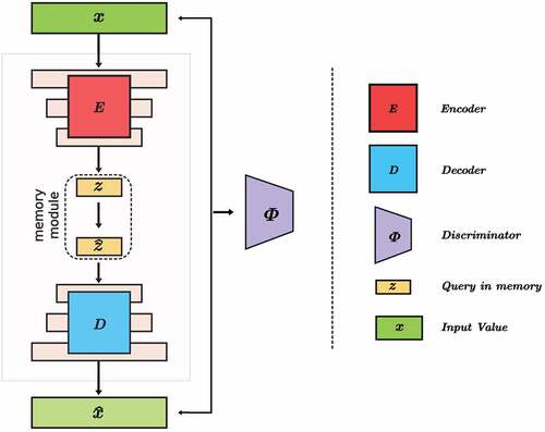
The defense model in Figure 2 is a system that is designed to protect against adversarial attacks on image classification models. It is composed of three main components: a generator, a discriminator, and a memory module. The generator is a combination of the encoder and decoder from an autoencoder, with the addition of three convolutional layers. The encoder processes the input image using convolutional techniques to extract higher-level characteristics, and encodes this information into a high-level latent encoding. This latent encoding is a compact representation of the input image that captures its important features. The decoder then restores the latent encoding back into an image using a deconvolution process. The memory module connects the first and second layers of the encoder to the second and third layers of the decoder, respectively. It is responsible for storing the information that is passed between these layers and allowing it to be used by the generator in the restoration process. Overall, the defense model works by first encoding the input image into a latent encoding using the encoder, storing this information in the memory module, and then using the decoder to restore the latent encoding back into an image. This restoration process helps to ensure that the output image is similar to the original input, even if it has been modified by an adversarial attack.

Figure 2. The network architecture of defense model used in this study.

Adversarial GAN

AdvGAN (Adversarial Generative Networks) is a type of generative model that is specifically designed to generate adversarial examples. The Adversarial GAN serves as an adversary, challenging the defense mechanism by generating adversarial examples. The AdvGAN model generates an adversarial example $G(x)$ from an original image by adding a new goal $(L_y=J_{\theta }(G(x);f(x)+\alpha )$ to the objective function $(LAdvGAN=L_y+\alpha LGAN)$ of the model. The new goal is defined as the difference between the prediction of the machine learning model for the original image and the prediction of the machine learning model for the adversarial example. The new goal is minimized using an optimization algorithm, such as stochastic gradient descent. The objective function of the AdvGAN model is a combination of the new goal and a regularization term. The regularization term is used to ensure that the adversarial example looks similar to the original image and that the adversarial example is generated using a smooth and continuous function. After training, the AdvGAN model should be able to generate an adversarial example $x^{\prime }$ that looks the same as the original image, but produces a prediction $f(x^{\prime })$ that differs from the prediction $f(x)$ for the original image by an amount $\mathrm{\Delta }$. The value of Delta depends on the strength of the adversarial attack and the robustness of the machine learning model.

The pixels of an image are first processed by a downsampling operation and then masked using the Pixel Scaling before being input to the input layer of a neural network. The purpose of the downsampling operation is to reduce the resolution of the image and the purpose of the masking operation is to selectively preserve or discard certain pixel values. The encoder is responsible for extracting a latent code $z$ from the input image, while the decoder is responsible for generating an output image from the latent code. In a traditional decoder architecture, the latent code is simply used as input to the first layer of the decoder and the output image is generated by cascading the output of each subsequent layer. However, when the decoder has more layers, the influence of the latent code decreases as it is passed upstream and the output image becomes increasingly reliant on the feature information provided by the skip link (a connection between the encoder and the decoder). This can lead to a decrease in the quality of the output images. To address this issue, we have included the latent code in each layer of the decoder. The extraction of latent codes from images involves obtaining a compact and lower-dimensional representation of an image, referred to as a latent code, that embodies the essential features and patterns contained within the image. This approach leverages the concept of unsupervised learning, where the objective is to learn a mapping from the high-dimensional pixel space to a lower-dimensional latent space that retains the critical information present in the image. This allows the latent code to have a more direct influence on the output image at each stage of the decoding process. The latent code is divided into three parts and each part is input to a different layer of the decoder. The first part is directly input to the first layer of the decoder, while the second and third parts are input to the second and third layers of the decoder after being connected to the features from the memory module (a component of the neural network that stores and retrieves information). This approach allows the latent code to have a more consistent influence on the output image, which should result in higher quality output images.

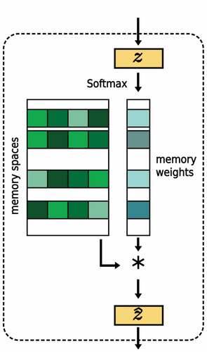
The memory module in our system uses several components to store the typical features of clean images. We use a softmax function to calculate the similarity score between each query and all the items before reading them. The softmax function is a widely used technique for computing the similarity score between two data sets. It involves the calculation of the exponential of the similarity score between each query-item pair, and subsequent normalization of these values by dividing them by the sum of all exponentials. This process results in a probability distribution over the items, wherein the relative similarity of each item to the query is reflected. Mathematically, given a set of items and a query, let the similarity score between the query and the $i-th$ item be represented by $s_i$. The softmax function (Bishop 2006) for this score is then defined as:

(3) $p_i=\frac{exp(s_i)}{\sum _{j=1}^{n}exp(s_j)}$(3)

where $p_i$ represents the probability of item $i$, $s_i$ represents the similarity score between the query and item $i$, and $n$ is the total number of items.

Each item is connected to multiple query vectors, which means that there may be several query vectors that are similar to it. Therefore, when updating items, we use all of the query vectors that are closest to the item. To update the memory, we use two operations: forget and update.

The forget operation functions by assigning a weight to each item in memory and subsequently multiplying it by a forget gate value between 0 and 1, thereby determining which information should be removed from memory. The forget gate value is indicative of the quantity of information from the corresponding memory item that ought to be discarded. This operation is essential in preventing memory overload with obsolete or irrelevant information. Conversely, the update operation determines the specific new information that should be added to the memory. This is done by assigning a weight to each candidate item and multiplying it by an update gate value between 0 and 1, indicating the proportion of the new information from the corresponding item that should be incorporated. The update operation is integral in accommodating new information and refreshing the memory.

In this case we work with Autoencoder. The Autoencoder with GAN takes this a step further by incorporating the adversarial information into the training process of the autoencoder, leading to a stronger defense.

Autoencoder with GAN

An autoencoder (Rumelhart, Hinton, and Williams 1986) is a type of neural network that is trained to reconstruct an input by learning to compress and then reconstruct the input data. It consists of two parts: an encoder, which maps the input data to a lower-dimensional representation called the latent space, and a decoder, which maps the latent representation back to the original input data. During training, the autoencoder is presented with a set of input samples and is asked to reconstruct them using the encoder and decoder. The goal of the autoencoder is to learn a function that can accurately reconstruct the input data from the latent representation. To measure the quality of the reconstruction, a reconstruction loss is used, which is a measure of the deviation between the input data and the reconstructed data. One issue with traditional autoencoder and the Variational AutoEncoder (VAE) (Kingma and Welling 2013), use a”pixel-level” reconstruction error such as the ${\mathrm{\ell }}_2$ distance or the log-likelihood to measure the deviation of the reconstructed samples from the input samples. The error can be too strict and result in overly smooth reconstructions. To address this issue, we add a discriminator to distinguish between the true input samples and the reconstructed samples. This helps to reduce blurriness and improve detail in the reconstruction, as the discriminator focuses on similarities in the overall distribution. The Memory Module is a key component that enables the defense mechanism to learn and retain information about the original data distribution, even in the presence of adversarial examples. By combining the autoencoder with adversarial training, we can improve the accuracy and detail of reconstructions while still being able to detect anomalies and defend against attacks.

Memory Module

To counteract against adversarial attack images that are designed to fool machine learning models, we can use a memory module to maintain a representation of normal patterns in the input data. The memory module consists of vectors, each of which represents a point on the normality manifold, which is a space that represents normal patterns in the input data. A normal pattern would be a pattern that is representative of the majority of the data points in the input data and is considered to be typical or expected. The normality manifold is a space that represents these normal patterns in the input data. During the reconstruction process, the encoder generates a query that retrieves vectors from the memory, which are then used to calculate the latent vector. By reconstructing the input data using the latent vector, we can ensure that the model is strictly reconstructing normal patterns. This can improve the model’s ability to detect and defend against adversarial attacks.

We utilized a neural network architecture that includes an encoder and a decoder. The encoder, represented by $f_e(\cdot )$, processes the input $\mathit{x}$ and generates a latent vector $\mathit{z}$. The decoder, denoted as $f_d(\cdot )$, takes the latent vector and converts it back into the input space to produce the reconstructed sample $\hat{\mathit{x}}$.

(4) $\begin{array}{rl}& \mathit{z}=f_e(\mathit{x}),\\ & \hat{\mathit{x}}=f_d(\hat{\mathbf{z}}).\end{array}$(4)

In a standard autoencoder, the latent vector z is used directly to obtain the reconstructed output, $\hat{\mathit{z}}=\mathit{z}$. However, in our approach, the latent vector z is transformed into a different latent vector, denoted as $\hat{z}$, using the memory module. The reconstruction error between the input sample and the reconstructed output is measured using various metrics, such as the Euclidean distance, ${\mathrm{\ell }}_2$.

(5) ${\mathcal{L}}_{\mathrm{r}\mathrm{e}\mathrm{c}}=\parallel \mathit{x}-\hat{\mathit{x}}{\parallel }_2$(5)

The objective of a standard autoencoder is to minimize the reconstruction error ${\mathcal{L}}_{\mathrm{r}\mathrm{e}\mathrm{c}}$. Autoencoder-based defense methods use the reconstruction error ${\mathcal{L}}_{\mathrm{r}\mathrm{e}\mathrm{c}}$ as a measure of defense effectiveness, with samples that have high reconstruction errors being considered adversarial images.

A common challenge with standard autoencoders is that the mean squared error (MSE) loss can cause reconstructions to be overly smooth. To address this issue, we utilize adversarial training. Specifically, we add a discriminator, represented by $\varphi (\cdot )$, to differentiate between the input samples and the reconstructions.

(6) ${\mathcal{L}}_{\mathrm{a}\mathrm{d}\mathrm{v}}={\mathbb{E}}_{\mathit{x}\sim p_{\mathrm{d}\mathrm{a}\mathrm{t}\mathrm{a}}(\mathit{x})}[log(\varphi (\mathit{x}))]+{\mathbb{E}}_{\hat{x}\sim p\mathrm{g}\mathrm{e}\mathrm{n}(\hat{\mathit{x}})}[log(1-\varphi (\hat{\mathbf{x}}))]$(6)

The distribution of the ground truth data is represented by $p_{\mathrm{d}\mathrm{a}\mathrm{t}\mathrm{a}}$, while the distribution of the reconstructed samples is represented by $p_{\mathrm{g}\mathrm{e}\mathrm{n}}$. Consequently the goal of training an autoencoder becomes:

(7) ${\mathcal{L}}_{\mathrm{f}\mathrm{u}\mathrm{l}\mathrm{l}-\mathrm{a}\mathrm{d}\mathrm{v}}={\mathcal{L}}_{\mathrm{a}\mathrm{d}\mathrm{v}}+\lambda \cdot {\mathcal{L}}_{\mathrm{r}\mathrm{e}\mathrm{c}}$(7)

The weight of the reconstruction objective is represented by $\lambda$ where the value ranging from 0.01 to 0.1. To maintain the structure of normal patterns, we enhance the autoencoder with a memory module. The latent vector that the decoder receives is created by combining different elements from the memory module. In the memory module shown in Figure 3, the vector produced by the encoder is used to determine the weights for the memory slots, which means that the memory module is responsible for capturing normal patterns instead of the encoder. The memory module is used consistently throughout the training process.

Figure 3. The memory module in the illustration is used to represent a set of memory vectors that represent what is considered normal. When reconstructing an input, the encoder’s output is used to determine the weights of each memory vector. The latent vector that is input into the decoder is created by combining the memory vectors using these weights.

The memory module consists of a matrix $\mathrm{M}=\left[{\mathit{m}}_1,\cdots ,{\mathit{m}}_M\right]\in {\mathbb{R}}^{M\times K}$ where $M$ is the size of the memory and $K$ is the dimension of each memory spot ${\mathit{m}}_i$. Given a query $\mathit{z}$, the latent vector $\hat{\mathit{z}}$ is computed through a linear combination of the memory spots:

(8) $\hat{\mathit{z}}=\sum _{i=1}^M{\mathit{w}}_i\cdot {\mathit{m}}_i=\mathit{w}\mathbf{M}.$(8)

In this case, the weight of the $i$-th memory slot ${\mathit{m}}_i$ in the overall memory is represented by the variable ${\mathit{w}}_i$. The query vector $\mathit{z}$, which is generated by the encoder and is equal to $\mathit{z}=f_e(\mathit{x})$, determines this contribution.

There are various ways to calculate the memory weights $\mathit{w}$. In this case, the normalized query vector is used directly as the memory weights. If the dimensions of the query and memory size do not match, the query is first mapped into the ${\mathbb{R}}^M$ space using the projection head $\psi (\cdot )$. It is used to calculate the weights for the memory slots by normalizing the query-memory similarities using the Softmax function. The purpose of the projection head is to help the network more effectively compare and retrieve relevant information from its memory, which can improve its overall performance.

(9) $\mathit{w}=\mathrm{S}\mathrm{o}\mathrm{f}\mathrm{t}\mathrm{m}\mathrm{a}\mathrm{x}(\psi (\mathit{z})).$(9)

To produce accurate reconstructions in the reconstruction task, the decoder is restricted to using representations that come from the normality manifold. To achieve this, the memory module needs to store the most typical normal patterns. This ensures that the decoder has access to high-quality information for recreating the input.

Experiment Results

Attack Injection and Success Against Autonomous Driving

The Nvidia DAVE-2 autonomous driving model is a well-known and widely used model that is implemented and trained using PyTorch. It consistently uses an input image size of $128\times 128$ pixels.

The Root Mean Square Error (RMSE) is used to measure the model’s error rate, and it is shown in the table. A default model that always predicts 0 for all frames on the test dataset has an RMSE of 0.20678. In contrast, the customized Nvidia DAVE-2 model has an RMSE of 0.1055, indicating a lower error rate.

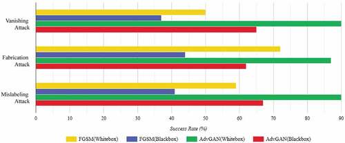
Two main types of environments in which experiments are conducted: Whitebox and Blackbox. In a Whitebox environment, the researchers have full knowledge of the driving model being used and can therefore create adversarial cases directly. In a Blackbox environment, attackers may try to train a proxy driving model offline and then use the AdvGAN model to perform Blackbox attacks. The effectiveness of adversarial attacks and countermeasures is measured by the attack success rate, which is calculated based on the number of successful attacks out of all adversarial examples. Successful Hijacking attacks are identified by steer angle deviation larger than 0.3, while the success of Vanishing, Fabrication, and Mislabeling attacks can be seen in the model’s output data in Figures 4, 5 and Figure 6, respectively. The success rate for these attacks is reported in Table 1.

Figure 4. In this scenario no adversarial attack is involved, so the driving model easily can detect the objects.

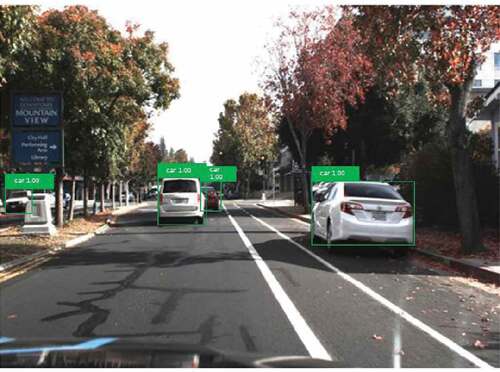
Figure 5. The following figures illustrate the effects of adversarial attacks on a detection system. (a) shows the results of a Vanishing attack, in which no objects can be detected. (b) shows the results of a Fabrication attack, in which the detection system returns a large number of falsely detected objects.

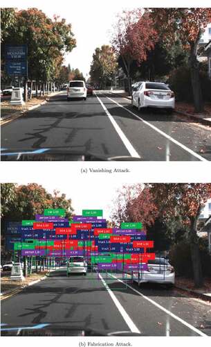
Figure 6. The figures illustrate the effects of adversarial attacks on the performance of a detection system. In Figure (a), all detected objects are incorrectly labeled with the same label as a result of the attack. Figure (b) demonstrates the effect of an attack in which objects with the same label are wrongly labeled with different labels.

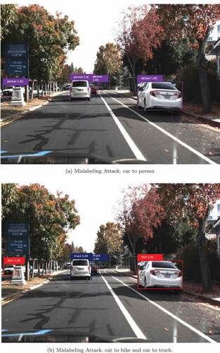
Table 1. Attack success rate in blackbox and whitebox setup.

Attack	Success Rate (Blackbox)	Success Rate (Whitebox)
Hijacking (FGSM)	26.4%	33.2%
Hijacking (AdvGAN)	87.7%	97.2%
Vanishing (FGSM)	37.34%	49.88%
Vanishing (AvdGAN)	64.71%	89.75%
Fabrication (FGSM)	44.23%	71.65%
Fabrication (AvdGAN)	61.84%	87.49%
Mislabeling (FGSM)	41.31%	58.88%
Mislabeling (AvdGAN)	67.05%	90.14%

According to Table 1, AvdGAN consistently outperforms FGSM in terms of success rate in adversarial situations. Within Whitebox setup, FGSM has a success rate of only $33.2\mathrm{\%}$ for the Hijacking Attack, while AvdGAN has a success rate of $97.2\mathrm{\%}$. This is because AvdGAN is able to learn and exploit the internal features of colored road lines, which can impact steer angle predictions and create adversarial disturbances. On Whitebox setup, FGSM has success rates of $49.88\mathrm{\%}$ and $71.65\mathrm{\%}$ for the Vanishing and Fabrication attacks, respectively, while AdvGAN has success rates of $89.75\mathrm{\%}$ and $87.49\mathrm{\%}$, respectively. Similarly, FGSM has a success rate of $58.88\mathrm{\%}$ for Mislabeling attacks during Whitebox setup, while AdvGAN has a success rate of $90.14\mathrm{\%}$. In the Blackbox setup, the Hijacking Attack with AdvGAN has the highest success rate, at $87.7\mathrm{\%}$, and AdvGAN outperforms FGSM in this case as well.

The Whitebox scenario depicted in Figure 7(a), the AdvGAN performs exceptionally well. It has a higher success rate than FGSM, which achieved a rate of $26.4\mathrm{\%}$. AdvGAN, on the other hand, achieved a rate of $87.7\mathrm{\%}$. These techniques generate adversarial perturbations that are tailored for specific models, and as a result, they are not as effective when used on different models.

Figure 7. Attack success rate for FGSM and AdvGAN attack in both whitebox and blackbox setup (Highjacking attack).

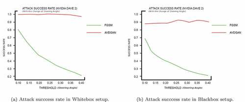
AdvGAN is more effective at attacking autonomous vehicles on Blackbox setup compared to FGSM, but its performance decreases when compared to the Whitebox setup. See Figure 7(b),. This suggests that adversarial attacks on autonomous vehicles are possible, raising concerns about their safety and the potential for the driving system to be compromised.

AdvGAN is a particularly dangerous attack because it can generate effective adversarial instances when attacking a model in a Whitebox setting. This is because AdvGAN leverages the properties of the targeted model to create its attacks. However, when tested in a Blackbox setting, the transferability of adversarial examples to driving models was not as strong. This suggests that the complexity of the network architecture of driving models may impact their vulnerability to adversarial attacks. In general, adversarial examples seem to be less successful at attacking autonomous driving models in a Blackbox setting. Figure 8 showing the successful attacks in Vanishing, Fabrication and Mislabeling attack.

Figure 8. Successful Attack for Vanishing, Fabrication and Mislabeling Attack.

Defense Performance Result – Proposed

We tested several defensive techniques, including Autoencoder, Block Switching, Adversarial Training, Defense Distillation, and Feature Squeezing, on FGSM and AdvGAN attacks, and compared their effectiveness with our proposed study.

From Table 2, we can see that the defense techniques of adversarial training, Defense Distillation, Feature Squeezing, and Autoencoder are not effective at defending against AdvGAN attacks in both Whitebox and Blackbox settings when applied to the Udacity dataset. However, the Block switching technique left minimal impact in terms of defense, though it does have an impact on the accuracy of the original image’s classification. Overall, it appears that adversarial training has poor generalization ability and is not able to withstand many attacks.

Table 2. Defense success rate in whitebox and blackbox setup.

Attacks	Mechanisms	Whitebox		Blackbox
(a) Hijacking	Defensive	FGSM	AdvGAN	FGSM	AdvGAN
	Autoencoder	78.4%	45.2%	45.4%	23.5%
	Block Switching	31.8%	17.3%	49.2%	37.3%
	Adversarial Training	89.7%	66.5%	50.1%	40.4%
	Defense Distillation	76.5%	45.3%	40.6%	25.7%
	Feature Squeezing	67.1%	54.2%	35.7%	31.6%
	Proposed	93.8%	91.2%	71.3%	63.1%
(b) Vanishing	Autoencoder	60.2%	40.4%	37.7%	26.1%
	Block Switching	20.1%	14.9%	56.2%	39.3%
	Adversarial Training	77.2%	65.5%	45.0%	39.3%
	Defense Distillation	58.3%	34.6%	33.8%	24.8%
	Feature Squeezing	51.7%	34.6%	33.4%	21.7%
	Proposed	63.97%	48.49%	71.43%	63.74%
(c) Fabrication	Autoencoder	44.5%	23.1%	23.3%	20.5%
	Block Switching	29.2%	17.5%	34.9%	25.8%
	Adversarial Training	50.4%	45.0%	33.7%	31.3%
	Defense Distillation	57.8%	30.9%	31.4%	25.5%
	Feature Squeezing	46.1%	35.4%	29.6%	30.1%
	Proposed	61.3%	52.2%	69.1%	60.0%
(d) Mislabeling	Autoencoder	59.3%	42.6%	35.9%	28.3%
	Block Switching	25.4%	24.8%	52.6%	36.6%
	Adversarial Training	65.4%	44.1%	34.4%	41.5%
	Defense Distillation	53.8%	38.9%	30.1%	26.6%
	Feature Squeezing	49.6%	29.2%	32.7%	24.5%
	Proposed	69.5%	57.7%	74.1%	64.4%

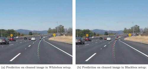
Our technique is not specifically designed to defend against any particular type of attack, but it has shown to be effective against a range of attacks. It is used to ensure high-quality reconstruction and to prevent the generation of disrupted images during the reconstruction phase. This helps to improve the model’s overall robustness while maintaining a high level of accuracy on unmodified images. As shown in Figure 9, the predicted trajectory of our model remains accurate even when applied to cleaned images.

Figure 9. Prediction of the cleaned image in both whitebox and blackbox setup.

Performance in Whitebox Setup

Table 2 (a) presents a comparison of the defense success rates of Blackbox and Whitebox setups against Hijacking attacks. The results indicate that, among the defense mechanisms examined, Autoencoder, Adversarial training, and Defense Distillation are most effective in defending against FGSM attacks in the Whitebox setup. Adversarial Training also performs well in protecting against AdvGAN attacks in this setup. Our proposed defense method demonstrated the highest success rate, achieving a defense rate of $93.8\mathrm{\%}$ against FGSM and $91.2\mathrm{\%}$ against AdvGAN.

Table 2 (b) illustrates the success rate of different defense methods against Vanishing attacks. In the Whitebox scenario, Adversarial Training outperformed our proposed method.

As demonstrated in Table 2 (c), the performance of our proposed method is lowest against Fabrication attacks. However, it still performs better than the other methods. It performs 3.5% better than Defense Distillation against FGSM attack in Whitebox scenario and 7.2% better than AdvGAN.

In this paper, we examine two types of mislabeling attacks. In order to evaluate the results, we calculated the average of the data. As depicted in Table 2 (c), our proposed method demonstrates the highest effectiveness in defending against mislabeling attacks in a whitebox configuration for both FGSM and AdvGAN, in comparison to vanishing and fabrication attacks.

Performance of Proposed Method – Blackbox Setup

In the Blackbox configuration, the most probable information that the attacker may possess is related to the classifier, leading to a lower defense success rate in comparison to the Whitebox setup. The Feature Squeezing method demonstrated insufficient performance, with a defense success rate of $35.7\mathrm{\%}$ against FGSM and $31.6\mathrm{\%}$ against AdvGAN. Other defense techniques, including Block switching, Adversarial Training, and Defense Distillation, exhibited defense success rates ranging from $40-50\mathrm{\%}$, which are also deemed inadequate in comparison to the proposed method. The proposed method exhibited superior performance, achieving a defense success rate of $71.3\mathrm{\%}$ against FGSM and $63.1\mathrm{\%}$ against AdvGAN.

The results presented in Table 2 (b), within the Blackbox configuration, indicate that the defense Vanishing attack achieved a success rate of $71.43\mathrm{\%}$ and $63.74\mathrm{\%}$, respectively. In contrast, our proposed study demonstrated superior performance in defending against Mislabeling attacks, as demonstrated in Table 2 (d).

The proposed method uses discrete memory addressing mechanisms to access stored information. Unlike traditional neural networks, which use continuous weights and activations, this method uses discrete memory addresses, making it non-differentiable and challenging to apply gradient-based optimization methods. In order to overcome the non-differentiability of our technique, we employed Adversarial training to estimate the gradient of the classifier. In the course of our experiments, we maintained consistency by utilizing the same attack parameters and datasets. The results of our experiments demonstrate that by training the purification model and the classifier concurrently through Adversarial training, our proposed strategy is successful in effectively defending against attacks from adversarial examples. As a consequence, the samples reconstructed by our model are highly similar to the original samples, thereby enhancing the robustness of the model without affecting its accuracy.

Time and Computation Overhead on Defense Mechanism

For our proposed experiment, we used python Jupyter Notebook 4.8 and Keras with TensorFlow as the backend. We did our experiment on an AMD Ryzen 5 5600 H CPU 3.30 GHz, 16 GB RAM, Windows 11 (64-bit), and NVIDIA GeForce RTX 3050.

Table 3 shows the impact of different defense strategies on Time (delay), GPU usage, and GPU memory. Adversarial Training and Defense Distillation have the longest Time overhead, with delays of $5.27s$ and $2.81s$, respectively. These approaches also have high GPU memory overhead, with Adversarial Training using more than $40\mathrm{\%}$ of GPU memory when predicting an attack. While the other defenses have low Time overhead and better GPU utilization and memory usage compared to Adversarial Training, our proposed method has a Time overhead of $0.743s$, $10\mathrm{\%}$ GPU utilization overhead, and $7.72\mathrm{\%}$ GPU memory overhead.

Table 3. Time and computation overhead on defense mechanism (Hijacking attack).

Defensive	Time Overhead (s)	GPU Overhead	GPU Overhead
		(Utilization %)	(Memory %)
Autoencoder	0.064	8	2.4
Block Switching	0.073	8	4.75
Adversarial Training	5.27	11	47.4
Defense Distillation	2.81	8	25.1
Feature Squeezing	0.0572	5	5.01
Proposed	0.743	10	7.72

Discussion

In this study, we aimed to explore the use of memory module with autoencoder as a defense mechanism against adversarial attacks in autonomous driving systems. Our results showed that the integration of the memory module significantly improves the performance of the autoencoder by enabling it to reduce false negatives during evaluation and prevent contamination of the encoded latent space with adversarial samples. The memory module helps the autoencoder to reconstruct a diverse range of adversarial attacks and provides a more robust and effective defense system for real-world applications.

One of the challenges in using autoencoders as a defense mechanism is the difficulty in learning representations for sequential and structured data. Traditional autoencoders lack the ability to store information about the data, making it challenging to effectively reconstruct adversarial attacks. The memory module in our system overcomes this challenge by providing an additional metric for evaluating reconstruction errors, allowing the autoencoder to identify and reconstruct a broader range of adversarial attacks.

The reconstruction task has been traditionally used as an effective method for detecting global adversarial samples. However, it may not consistently identify local perturbations or contextual deviations, particularly when the values are within the bounds of normality. By integrating the reconstruction task with the memory module, the autoencoder is able to effectively detect a wider range of adversarial attacks, making the defense system more robust and effective for real-world applications. Figure 10 clearly shows struggle without the memory module.

Figure 10. Evaluating and comparing the performance of memory module-based model in different setups.

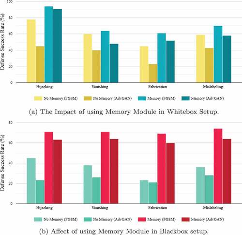
The results of the defense success rates against various types of attacks in whitebox and blackbox setups were analyzed and compared. In the case of Hijacking attacks, the proposed mechanism achieved the highest defense success rate with 93.8% against FGSM and 91.2% against AdvGAN in the whitebox setup, and 71.3% against FGSM and 63.1% against AdvGAN in the blackbox setup. In the case of vanishing attacks, the proposed mechanism showed a defense success rate of 63.97% in the whitebox and 71.43% in the blackbox against FGSM, and 48.49% in the whitebox and 63.74% in the blackbox against AdvGAN. In the case of fabrication attacks, the proposed mechanism outperformed with a defense success rate of 61.3% in the whitebox and 69.1% in the blackbox against FGSM, and 52.2% in the whitebox and 60.0% in the blackbox against AdvGAN. The proposed mechanism also performed the best in defending against Mislabeling Attacks, with a defense success rate of 69.5% in the whitebox and 74.1% in the blackbox against FGSM and AdvGAN, respectively.

In comparison, Adversarial Training also showed good performance, but its defense success rate dropped in the blackbox scenario. The autoencoder mechanism had a lower success rate compared to the proposed mechanism in all the attacks. Defense Distillation and Feature Squeezing performed poorly in both setups, while Block Switching showed slightly better results against FGSM in the blackbox setup. Overall, the proposed mechanism demonstrated superior performance in defending against various attacks, outperforming the other mechanisms, including autoencoder, adversarial training, defense distillation, feature squeezing, and block switching, in both whitebox and blackbox setups.

Despite its advantages, our system still faces some limitations. The defense success rate of the system varies substantially across different attacks, and the system incurs a significant computational cost due to a high time and GPU overhead value. Future research could focus on conducting experiments utilizing advanced autonomous driving models in real-time scenarios to further evaluate the effectiveness of the system and identify potential areas for optimization.

In the future, potential areas for improvement of the memory module with autoencoder system for adversarial defense in autonomous driving systems could include reducing computational costs through more efficient memory storage techniques or reducing the number of parameters in the memory module. Another area to explore is incorporating other defense mechanisms, such as adversarial training or generative models, to further enhance the robustness of the system. Further validation of the system’s effectiveness can be achieved by conducting experiments with larger and more complex datasets, as well as evaluating its performance against multiple concurrent adversarial attacks, which are likely to occur in real-world scenarios. Additionally, investigating the system’s performance against adversarial attacks generated through various methods and under different conditions, such as targeted versus untargeted attacks, can provide insights into its robustness. Lastly, the potential for transfer learning, where the memory module could be trained on one autonomous driving system and transferred to another, could also be explored to improve the defense performance.

In conclusion, the incorporation of the memory module into our autoencoder system represents a significant advancement in the field of adversarial defense. By leveraging the additional information provided by the memory module, the autoencoder is able to effectively defend against a broader range of adversarial attacks and provide a more robust and effective defense system for real-world applications.

Conclusion

In this research, we propose a new method for defending autonomous driving models against adversarial attacks and compare it to other common defense systems. We test the effectiveness of our approach using four adversarial attacks in both Whitebox and Blackbox scenarios. Our defense method uses a memory module to encode the normal behavior of the model into memory vectors. By combining these vectors, reconstructions are only calculated based on typical patterns. We conducted experiments on a real-world driving dataset and found that our method performs better than other baselines in terms of effectiveness and robustness. In the Whitebox scenario, our defense had success rates of $93.8\mathrm{\%}$ and $91.2\mathrm{\%}$. The result is $4.1\mathrm{\%}$ and $24.7\mathrm{\%}$ better than Adversarial Training. Adversarial Training is the preceding optimum outcome from this experiment. In the Blackbox scenario, the success rates were $64.4\mathrm{\%}$ and $74.1\mathrm{\%}$. These are $22.9\mathrm{\%}$ better than Adversarial Training and $21.5\mathrm{\%}$ better than Block Switching. Both of these provided the prior optimal results. Our results show that this method significantly improves the model’s ability to correctly classify adversarial cases.

Acknowledgements

Part of this study was funded by the ICSCoE Core Human Resources Development Program and MEXT Scholarship, Japan.

Disclosure statement

No potential conflict of interest was reported by the authors.

References

- Bishop, C. M. 2006. Pattern recognition and machine learning. New York: Springer.
- Bojarski, M., D. Del Testa, D. Dworakowski, B. Firner, B. Flepp, P. Goyal, L. D. Jackel, M. Monfort, U. Muller, J. Zhang et al. 2016. End to end learning for self-driving cars. arXiv preprint arXiv 1604:07316.
- Buckman, J., A. Roy, C. Raffel, and I. Goodfellow. 2018. “Thermometer encoding: One hot way to resist adversarial examples.” In International Conference on Learning Representations, Vancouver.
- Chow, K.H., L. Liu, M. Loper, J. Bae, M. Emre Gursoy, S. Truex, W. Wei, and W. Yanzhao 2020. “Adversarial objectness gradient attacks in real-time object detection systems.” In 2020 Second IEEE International Conference on Trust, Privacy and Security in Intelligent Systems and Applications (TPS-ISA), Atlanta, 263–1007.
- Chung, J., C. Gulcehre, K. Cho, and Y. Bengio. 2014. Empirical evaluation of gated recurrent neural networks on sequence modeling. arXiv preprint arXiv 1412:3555.
- Elliott, D., W. Keen, and L. Miao. 2019. Recent advances in connected and automated vehicles. Journal of Traffic and Transportation Engineering (English Edition) 6 (2):109–31. https://www.sciencedirect.com/science/article/pii/S2095756418302289.
- Gong, D., L. Liu, L. Vuong, B. Saha, M. Reda Mansour, S. Venkatesh, and A. van den Hengel. 2019. “Memorizing normality to detect anomaly: Memory-augmented deep autoencoder for unsupervised anomaly detection.” In Proceedings of the IEEE/CVF International Conference on Computer Vision, Seoul, 1705–14.
- Goodfellow, I. J., J. Shlens, and C. Szegedy. 2014a. Explaining and harnessing adversarial examples. arXiv preprint arXiv 1412:6572.
- Goodfellow, I. J., J. Shlens, and C. Szegedy. 2014b. Intriguing properties of neural networks. arXiv preprint arXiv 1312:6199.
- Guo, C., M. Rana, M. Cisse, and L. Van Der Maaten. 2017. Countering adversarial images using input transformations. arXiv preprint arXiv 1711: 00117.
- Hochreiter, S., and J. Schmidhuber. 1997. Long short-term memory. Neural Computation 9 (8):1735–80. doi:10.1162/neco.1997.9.8.1735.
- Huang, S., N. Papernot, I. Goodfellow, Y. Duan, and P. Abbeel. 2017. Adversarial attacks on neural network policies. arXiv preprint arXiv 1702:02284.
- Jain, L. C., and L. R. Medsker. 1999. Recurrent neural networks: design and applications. 1st ed. USA: CRC Press, Inc.
- Jalal, A., A. Ilyas, C. Daskalakis, and A. G. Dimakis. 2017. The robust manifold defense: Adversarial training using generative models. arXiv preprint arXiv 1712:09196.
- Kaiming, H., H. Fan, W. Yuxin, S. Xie, and R. Girshick. 2020. “Momentum contrast for unsupervised visual representation learning.” In Proceedings of the IEEE/CVF conference on computer vision and pattern recognition, Seattle, 9729–38.
- Kingma, D. P., and M. Welling. 2013. Auto-encoding variational bayes. arXiv preprint arXiv 1312:6114.
- Liu, W., X. Daniel Wang, and D. Song. 2015. “Feature squeezing: Detecting adversarial examples in deep neural networks.” In 2015 IEEE Symposium on Security and Privacy, 567–76. San Jose: IEEE.
- MordorIntelligence. 2021. “AUTONOMOUS (DRIVERLESS) CAR MARKET - GROWTH, TRENDS, COVID-19 IMPACT, and FORECASTS (2023 - 2028).” Accessed December 29, 2022 https://www.mordorintelligence.com/industry-reports/autonomous-driverless-cars-market-potential-estimation.
- Pang, L., X. Yuan, S. Jiantao, and L. Hongyang 2020. “Block switching defenses are not robust to adversarial examples.” In International Conference on Learning Representations, Addis Ababa.
- Papernot, N., P. McDaniel, I. Goodfellow, S. Jha, Z. Berkay Celik, and A. Swami. 2017. “Practical black-box attacks against machine learning.” In Proceedings of the 2017 ACM on Asia conference on computer and communications security, Abu Dhabi, 506–19.
- Papernot, N., P. McDaniel, X. Wu, S. Jha, and A. Swami. 2016. “Distillation as a defense to adversarial perturbations against deep neural networks.” In 2016 IEEE symposium on security and privacy (SP), 582–97. San Jose: IEEE.
- Park, H., J. Noh, and B. Ham. 2020. “Learning memory-guided normality for anomaly detection.” In Proceedings of the IEEE/CVF Conference on Computer Vision and Pattern Recognition, Seattle, 14372–81.
- Pomerleau, D. A. 1988. Advances in Neural Information Processing Systems 1.
- Ruder, S. 2016. An overview of gradient descent optimization algorithms. arXiv preprint arXiv 1609:04747.
- Rumelhart, D. E., G. E. Hinton, and R. J. Williams. 1986. Learning representations by back-propagating errors. Nature 323 (6088):533–36. doi:10.1038/323533a0.
- Samangouei, P., M. Kabkab, and R. Chellappa. 2018. Defense-gan: Protecting classifiers against adversarial attacks using generative models. arXiv preprint arXiv 1805:06605.
- Shixiang, G., and L. Rigazio. 2014. Towards deep neural network architectures robust to adversarial examples. arXiv preprint arXiv 1412:5068.
- Song, Y., T. Kim, S. Nowozin, S. Ermon, and N. Kushman. 2017. “Pixeldefend: Leveraging generative models to understand and defend against adversarial examples.” arXiv preprint arXiv:1710.10766.
- Tramèr, F., A. Kurakin, N. Papernot, I. Goodfellow, D. Boneh, and P. McDaniel. 2017. “Ensemble adversarial training: Attacks and defenses.” arXiv preprint arXiv:1705.07204.
- Udacity, A. R. 2017. “Udacity self-driving car dataset.”
- Wang, W., Y. Huang, Y. Wang, and L. Wang. 2014. “Generalized autoencoder: A neural network framework for dimensionality reduction.” In Proceedings of the IEEE conference on computer vision and pattern recognition workshops, Columbus, 490–97.
- Zhirong, W., Y. Xiong, S. X. Yu, and D. Lin. 2018. “Unsupervised feature learning via non-parametric instance discrimination.” In Proceedings of the IEEE conference on computer vision and pattern recognition, Salt Lake City, 3733–42.
- Zhou, J., C. Liang, and J. Chen. 2020. “Manifold projection for adversarial defense on face recognition.” In European Conference on Computer Vision, 288–305. Glasgow: Springer.