Physical Domain Reconstruction with Finite Volume Neural Networks

ABSTRACT

The finite volume neural network (FINN) is an exception among recent physics-aware neural network models as it allows the specification of arbitrary boundary conditions (BCs). FINN can generalize and adapt to various prescribed BC values not provided during training, where other models fail. However, FINN depends explicitly on given BC values and cannot deal with unobserved parts within the physical domain. To overcome these limitations, we extend FINN in two ways. First, we integrate the capability to infer BC values on-the-fly from just a few data points. This allows us to apply FINN in situations, where the BC values, such as the inflow rate of fluid into a simulated medium, are unknown. Second, we extend FINN to plausibly reconstruct missing data within the physical domain via a gradient-driven spin-up phase. Our experiments validate that FINN reliably infers correct BCs, but also generates smooth and plausible full-domain reconstructions that are consistent with the observable data. Moreover, FINN can generate precise predictions orders of magnitude more accurate compared to competitive pure ML and physics-aware ML models – even when the physical domain is only partially visible, and the BCs are applied at a point that is spatially distant from the observable volumes.

Introduction

Physics-informed machine learning approaches incorporate physical knowledge as inductive bias (Battaglia et al. 2018). When applied to corresponding physical domains, they yield improvements in generalization and data efficiency when contrasted with pure machine learning (ML) systems (Karlbauer et al. 2021; Raissi, Perdikaris, and Karniadakis 2019). Moreover, inductive biases often help ML models to play down their “technical debt” (Sculley et al. 2015), effectively reducing model complexity while improving model explainability. Several recently proposed approaches augment neural networks with physical knowledge (Le Guen and Thome 2020; Li et al. 2020; Long et al. 2018; Seo, Meng, and Liu 2019; Sitzmann et al. 2020).

But these models do neither allow including – or structurally capturing – explicitly defined physical equations, nor do they generalize to unknown initial or boundary conditions (Raissi, Perdikaris, and Karniadakis 2019). The recently introduced finite volume neural network (FINN) (Karlbauer et al. 2022; Praditia et al. 2021, 2022) accounts for both: it combines the learning abilities of artificial neural networks with physical and structural knowledge from numerical simulations by modeling partial differential equations (PDEs) in a mathematically compositional manner. So far, FINN is the only physics-aware neural network that can handle boundary conditions that were not considered during training. Nonetheless, boundary conditions (BCs) need to be known and presented explicitly. But not even FINN can predict processes where unknown boundary conditions apply. In realistic application scenarios, however, a quantity of interest is measured for a specific, limited region only. The amount of the quantity that flows into the observed volumes through boundaries is notoriously unknown and hitherto impossible to predict. On top of that, the available systems are not able to expand their predictions beyond the boundaries of the observable volumes. One example of relevance is weather forecasting: a prediction system observes, e.g., precipitation or cloud density for a limited area. Incoming weather dynamics from outside of the observed region that strongly control the processes inside the domain cannot be incorporated, turning into one of the main error sources in numerical simulations.

Here, we expand on previous work by Can Horuz et al. (2022), which presented an approach to infer the explicitly modeled BC values of FINN on-the-fly, while observing a particular spatiotemporal process. The approach is based on the retrospective inference principle (Butz et al. 2019; Otte, Karlbauer, and Butz 2020), which applies a prediction error-induced gradient signal to adapt the BC values of a trained FINN model. Only very few data points are required to find boundary conditions that best explain the recently observed process dynamics and, moreover, to predict the observed process with high accuracy in closed-loop. We compare the quality of the inferred boundary conditions and the prediction error of FINN with two state-of-the-art architectures, namely, DISTANA (Karlbauer et al. 2020) and PhyDNet (Le Guen and Thome 2020).

The distributed spatiotemporal graph artificial neural network architecture (DISTANA) is a hidden state inference model for time-series prediction. It encodes two different kernels in a graph structure: First, the prediction kernel (PK) network predicts the dynamics at each spatial position while being applied to each node of the underlying mesh. Second, the transition kernel (TK) network coordinates the lateral information flow between PKs, thus allowing the model to process spatiotemporal data. The PKs consist of feed-forward neural networks combined with long short-term memory (LSTM) units (Hochreiter and Schmidhuber 1997). Similar to Karlbauer et al. (2020), we use just linear mappings as TKs in this work since the data considered here is represented on a regular grid and does not require a more complex processing of lateral information. All PKs and TKs share weights. DISTANA has been shown to perform better compared to convolutional neural networks (CNN), recurrent neural networks (RNN), convolutional LSTM, and similar models (Karlbauer et al. 2020, 2021). The model’s performance and its applicability to spatiotemporal data makes it a suitable pure ML baseline for this paper.

PhyDNet is a physics-aware encoder-decoder model. First, it encodes the input at time step $t$. Afterward, the encoded information is disentangled into two separate networks, PhyCell and ConvLSTM-Cell. Inspired from physics, PhyCell implements spatial derivatives up to a desired order and can approximate solutions of a wide range of PDEs, e.g., heat equation, wave equation, and the advection-diffusion equation. Moreover, the model covers the residual information that is not subsumed by the physical norms. Concretely, the ConvLSTM-Cell complements the PhyCell and approximates the residual information in a convolutional deep learning fashion. The outputs of the networks are combined and fed into a decoder in order to generate a prediction of the unknown function at time $t+1$ (Le Guen and Thome 2020). PhyDNet is a state-of-the-art physics-aware neural network, which is applicable to advection-diffusion equations and was therefore selected as a physics-aware baseline in this study.

Our results indicate that FINN is the only architecture that reliably infers BC values and outperforms all competitors in predicting non-linear advection-diffusion-reaction processes when the BC values are unknown. As an extension to Can Horuz et al. (2022), we additionally hide 40% of the data that connect the boundaries with the simulation domain and demonstrate FINN’s ability to accurately infer this hidden information in agreement with the boundary condition.

Finite Volume Neural Network

The finite volume neural network (FINN) introduced in (Karlbauer et al. 2022; Praditia et al. 2021) is a physics-aware neural network model that combines the well-established finite volume method (FVM) (Moukalled, Mangani, and Darwish 2016) as an inductive bias with the learning abilities of deep neural networks. FVM discretizes a continuous partial differential equation (PDE) spatially into algebraic equations over a finite number of control volumes. These volumes have states and exchange fluxes via a clear mathematical structure. The enforced physical processing within the FVM structure constrains FINN to implement (partially) known physical-laws, resulting in an interpretable, well-generalized, and robust method.

Architecture

FINN solves PDEs that express non-linear spatiotemporal advection-diffusion-reaction processes, formulated in Karlbauer et al. (2022) as

(1) $\frac{\mathrm{\partial }u}{\mathrm{\partial }t}=D(u)\frac{{\mathrm{\partial }}^{2}u}{\mathrm{\partial }{x}^2}-v(u)\frac{\mathrm{\partial }u}{\mathrm{\partial }x}+q(u),$(1)

where $u$ is the unknown function of time $t$ and spatial coordinate $x$, which encodes a state. The objective of a PDE solver (if the PDE was fully known) is to find the value of $u$ in all time steps and spatial locations. However, Equation 1(1) $\frac{\mathrm{\partial }u}{\mathrm{\partial }t}=D(u)\frac{{\mathrm{\partial }}^{2}u}{\mathrm{\partial }{x}^2}-v(u)\frac{\mathrm{\partial }u}{\mathrm{\partial }x}+q(u),$(1) is composed of three, often unknown functions, which modify $u$, i.e., $D$, $v$, and $q$. $D$ is the diffusion coefficient, which controls the equilibration between high and low concentrations, $v$ is the advection velocity, which represents the movement of concentration due to the bulk motion of a fluid, and $q$ is the source/sink term, which increases or decreases the quantity of $u$ locally.

These unknown functions are approximated by neural network modules, which imitate the structure of Equation 1(1) $\frac{\mathrm{\partial }u}{\mathrm{\partial }t}=D(u)\frac{{\mathrm{\partial }}^{2}u}{\mathrm{\partial }{x}^2}-v(u)\frac{\mathrm{\partial }u}{\mathrm{\partial }x}+q(u),$(1) while applying it to a set of spatially discretized control volumes. Figure 1 and Equation 2(2) $\frac{\mathrm{\partial }{u}_i}{\mathrm{\partial }t}=\underset{S_i}{\underbrace{\underset{F_i=f_{i-}+f_{i+}}{\underbrace{\stackrel{\phi D}{\overbrace{D(u_i)}}\stackrel{\genfrac{}{}{0ex}{}{\phi N_{i-}}{\genfrac{}{}{0ex}{}{+}{\phi N_{i+}}}}{\overbrace{\frac{{\mathrm{\partial }}^2{u}_i}{\mathrm{\partial }{x}^2}}}-\stackrel{\genfrac{}{}{0ex}{}{\phi N_{i-}}{\genfrac{}{}{0ex}{}{or}{\phi N_{i+}}}}{\overbrace{\frac{\mathrm{\partial }{u}_i}{\mathrm{\partial }x}}}}}+\stackrel{\mathrm{\Phi }\psi }{\overbrace{q(u_i)}}}}$(2) illustrate how FINN models the PDE for a single control volume $i$. The first- and second-order spatial derivatives $\left(\frac{\mathrm{\partial }u}{\mathrm{\partial }x},\frac{{\mathrm{\partial }}^{2}u}{\mathrm{\partial }{x}^2}\right)$, for example, can be approximated with a linear layer, ${\phi }_{\mathcal{N}}$, aiming to learn the FVM stencil, i.e., the exchange terms between adjacent volumes. In the current work, the first-order flux multiplier (i.e., advection velocity) is approximated by neural networks which take $u$ as input. This applies to both Allen–Cahn and Burgers’ benchmarks and the networks have the size $[1,10,20,10,1]$, which makes 420 parameters (422 if BCs are learnt in the training as in Section 4.2).

Figure 1. The composition of the modules to represent and learn different parts of an advection-diffusion equation. Red lines indicate gradient flow during training and retrospective inference. Figure from Karlbauer et al. (2022).

(2) $\frac{\mathrm{\partial }{u}_i}{\mathrm{\partial }t}=\underset{S_i}{\underbrace{\underset{F_i=f_{i-}+f_{i+}}{\underbrace{\stackrel{\phi D}{\overbrace{D(u_i)}}\stackrel{\genfrac{}{}{0ex}{}{\phi N_{i-}}{\genfrac{}{}{0ex}{}{+}{\phi N_{i+}}}}{\overbrace{\frac{{\mathrm{\partial }}^2{u}_i}{\mathrm{\partial }{x}^2}}}-\stackrel{\genfrac{}{}{0ex}{}{\phi N_{i-}}{\genfrac{}{}{0ex}{}{or}{\phi N_{i+}}}}{\overbrace{\frac{\mathrm{\partial }{u}_i}{\mathrm{\partial }x}}}}}+\stackrel{\mathrm{\Phi }\psi }{\overbrace{q(u_i)}}}}$(2)

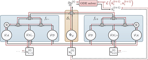
Furthermore, and in order to account for the structure of Equation 1(1) $\frac{\mathrm{\partial }u}{\mathrm{\partial }t}=D(u)\frac{{\mathrm{\partial }}^{2}u}{\mathrm{\partial }{x}^2}-v(u)\frac{\mathrm{\partial }u}{\mathrm{\partial }x}+q(u),$(1) , FINN introduces two kernels that are applied to each control volume with index $i$; similar to how convolution kernels are shifted over an input image. First, the flux kernel $\mathcal{F}=f_{-}+f_{+}$ models both the diffusive $D(u)\frac{{\mathrm{\partial }}^{2}u}{\mathrm{\partial }{x}^2}$ and the advective flux $v(u)\frac{\mathrm{\partial }u}{\mathrm{\partial }x}$, respectively, via the feedforward network modules ${\phi }_{\mathcal{D}}$ and ${\phi }_{\mathcal{A}}$. Second, the state kernel $\mathcal{S}$ models the source/sink term $q$ for each volume. All modules’ outputs are summed up to conclude in $\frac{\mathrm{\partial }u}{\mathrm{\partial }t}$, which results in a system of ODEs with respect to time that is solved by NODE (Chen et al. 2018). Accordingly, FINN predicts $u$ in time step $(t+1)$, that is ${\hat{u}}^{(t+1)}$, and the error is computed via $\mathcal{L}\left({\hat{u}}_i^{(t+1)},u_i^{(t+1)}\right)$, where $i$ corresponds to the discretized spatial control volume index and $\mathcal{L}$ is the mean squared error. FINN operates entirely in a closed-loop manner, i.e., only the initial condition $u^{(t=0)}$ is fed into the model to unroll a prediction ${\hat{u}}^{(1:T)}$ into the future, with sequence length $T$. Note that learning the diffusive flux has been demonstrated in earlier studies (Karlbauer et al. 2022; Praditia et al. 2021) and is not part of this work. Therefore, instead of approximating $D(u)$ by a neural network ${\phi }_{\mathcal{D}}$, we set it to the actual value used for data generation.

The connection scheme of different kernels and modules ensures compliance with fundamental physical rules, such that advection can spatially propagate exclusively to the left or to the right ($\mathcal{R}$ in Figure 1). Note that we only consider one-dimensional problems in this work, although FINN can also be applied to higher-dimensional equations. The reader is referred to Karlbauer et al. (2022) and Praditia et al. (2021) for an in-depth depiction of the model.

Boundary Condition Inference

The specification of boundary conditions (BCs) is required to obtain a unique solution of a PDE. Common BCs are Dirichlet (fixed values for $u$), periodic (any quantity leaving the field on one side enters on the opposing side), or Neumann (the derivative of $u$ is specified at the boundary). In contrast to state-of-the-art physics-aware neural networks (Le Guen and Thome 2020; Long et al. 2018; Raissi, Perdikaris, and Karniadakis 2019; Yin et al. 2021), FINN allows the explicit formulation of a desired BC. Thus, FINN can deal with not only simple boundary conditions (Dirichlet or periodic) but also more complicated ones such as Neumann (Karlbauer et al. 2022).

FINN uses the boundary conditions strictly. The solid implementation of a BC type (Dirichlet, periodic, Neumann) enables the model to read out unknown/unseen BC values of a given dataset. So far, however, it was necessary to use explicit BCs for solving a PDE. However, due to the explicit integration of BCs into the formulation of FINN, it is predestined to learn which BC values best describe a specific dataset – during both training and prediction. Here, we show that it is possible to infer not only BC values in a much larger range via retrospective inference, but also to recover parts of the simulation domain that were unavailable to the model during training.

From a broader perspective, the need for BCs is often a modeling artifact for real-world problems – simply because we do not have the means to simulate an entire system but need to restrict ourselves to a bounded subdomain. Even if these boundaries do not exist in the original system, our resulting model needs to identify their conditions for accurate forecasting. Our aim is to infer appropriate BCs and their values quickly, accurately, and reliably. Technically, a BC value is inferred by setting it as a learnable parameter and projecting the prediction error over a defined temporal horizon onto this parameter. Intuitively, the determination of the BC values can thus be described as an optimization problem where, instead of the network weights, the BC values are subject to optimization.

Benchmark PDEs

We performed experiments on two different PDEs and will first introduce these equations and later report the respective experiments and results.

Burgers’ Equation

Burgers’ equation is frequently used in different research fields to model, e.g., fluid dynamics, nonlinear acoustics, or gas dynamics (Fletcher 1983; Naugolnykh et al. 2000). It offers a useful toy example formulated as a 1D equation in this work as

(3) $\frac{\mathrm{\partial }u}{\mathrm{\partial }t}=-v(u)\frac{\mathrm{\partial }u}{\mathrm{\partial }x}+D\frac{{\mathrm{\partial }}^{2}u}{\mathrm{\partial }{x}^2},$(3)

where $u$ is the unknown function and $v(u)$ is the advective velocity, which is defined as an identity function $v(u)=u$ here. The diffusion coefficient $D$ is set to $0.01/\pi$ for data generation. During training, Burgers’ equation has constant values on the left and right boundaries defined as $u(-1,t)=u(1,t)=0$. However, these were modified to take different symmetric values at inference in order to assess the ability of the different models to cope with such variations. The initial condition is defined as $u(x,0)=-sin(\pi x)$.

Allen–Cahn Equation

Allen–Cahn is chosen and also defined as a 1D equation that could have periodic or constant boundary conditions. It is typically applied to model phase-separation in multi-component alloy systems and has also been used by Raissi, Perdikaris, and Karniadakis (2019) to analyze the performance of their physics-informed neural network (PINN). The equation is defined as

(4) $\frac{\mathrm{\partial }u}{\mathrm{\partial }t}=D\frac{{\mathrm{\partial }}^{2}u}{\mathrm{\partial }{x}^2}+R(u),$(4)

where the reaction term takes the form $R(u)=5u-5u^3$. The diffusion coefficient is set to $D=0.05$, which is significantly higher than in Karlbauer et al. (2022), where it was set to $D={10}^{-4}$. The reason for this decision is to scale up the diffusion relative to the reaction, such that the effects of the BCs are more apparent.

Experiments

We have conducted three different experiments. First, the ability to learn BC values during training is studied in Section 4.1. Afterward, we analyze the ability of the pre-trained models to infer unknown BC values in Section 4.2. Finally, in Section 4.3, we investigate the ability of the models to reconstruct 40% of the simulation domain while still inferring the BC of the dataset. Data were generated by numerical simulations using the Finite Volume Method, similarly to Karlbauer et al. (2022).

Learning with Fixed Unknown Boundary Conditions

This experiment is conducted in order to discover whether it is possible for the model to approximate the boundary conditions of the given dataset. It can be utmost useful in real-world scenarios to determine the unknown BC values during training, where the model determines the BC values according to the data without depending on prior assumptions.

The shape of the generated training data was $(256,49)$, where $N_x=49$ specifies the discretized spatial locations and $N_t=256$ the number of simulation steps. To train the models, we used the first 30 time steps of the sequence. The extrapolation data (remaining 226 time steps) is used to compute the test error. The learnt BC values are shown in Table 1 that neither DISTANA nor PhyDNet can deduce reasonable BC values.

Table 1. Comparison of the training error, test error, and the learnt BC values of all models. For each trial, the average results over 5 repeats are presented. Burgers’ dataset BC $=[1.0,-1.0]$ and Allen–Cahn dataset BC $=[-1.0,1.0]$.

Eqn.	Model	Training Error	Test Error	Learnt BC
Burgers’	DISTANA	$(4.6\pm 3.0)\cdot {10}^{-4}$	$1.69\pm 1.14$	$[0.5460\pm 0.0582,-0.5179\pm 0.0455]$
	PhyDNet	$(2.2\pm 0.5)\cdot {10}^{-5}$	$0.11\pm 0.07$	$[0.3735\pm 0.3259,-0.4068\pm 0.1849]$
	FINN	$(9.6\pm 9.9)\cdot {10}^{-8}$	$5\pm 4\cdot {10}^{-4}$	$[1.0004\pm 0.0002,-1.0004\pm 0.0002]$
Allen–Cahn	DISTANA	$(1.7\pm 2.2)\cdot {10}^{-4}$	$1.50\pm 1.67$	$[-0.5573\pm 0.0372,0.5293\pm 0.0149]$
	PhyDNet	$(6.4\pm 3.1)\cdot {10}^{-6}$	$0.16\pm 0.03$	$[-0.5060\pm 0.0858,0.4438\pm 0.0898]$
	FINN	$(3.4\pm 4.5)\cdot {10}^{-7}$	$1\pm 1\cdot {10}^{-4}$	$[-0.9955\pm 0.0049,0.9994\pm 0.0006]$

The results imply that the complex nature of the equations combined with large ranges of possible BC values indeed yields a challenging optimization problem, in which gradient-based approaches can easily get stuck in local minima. For example, the fact that FINN uses NODE (Chen et al. 2018) to integrate the ODE may lead to the convergence into a stiff system and, hence, unstable solutions. Moreover, as FINN employs backpropagation through time (BPTT), it can easily produce vanishing/exploding gradients. During preliminary studies, however, we realized that FINN benefits from shorter sequences in this regard. Thus, only the first 30 time steps of the data are employed. As a result, FINN identifies the correct BCs and – although this was not necessarily the goal – even yields a lower test error.

Neither PhyDNet nor DISTANA provide the option to meaningfully represent boundary conditions. Accordingly, the BCs are fed explicitly into the model on the edges of the simulation domain. The missing inductive bias of how to use these BC values, however, seemed to prevent the models to determine the correct BC (c.f. Table 1). Nevertheless, both PhyDNet and DISTANA can approximate the equation fairly accurately (albeit not reaching FINN’s accuracy), even when the determined BC values deviate from the true values. The learnt BC values by the two models do not converge to any point and persist around the initial values, which are $[0.5,-0.5]$ for Burgers’ and $[-0.5,0.5]$ for Allen–Cahn. Similarly, they remain around 0 when we set the initial BC values to $0$. We conclude that PhyDNet and DISTANA do not seem to consider the BC values.

On the other hand, FINN appears to benefit from the structural knowledge about BCs when determining their values. The BC values in Table 1 converged from $[4.0,-4.0]$ to $[1.0,-1.0]$, well maintaining them for the rest of the training (c.f. first row of Figure 2). As it can be seen on the second row of Figure 2, FINN also manages to infer BC values for Allen–Cahn in a larger range. In Figure 2, FINN demonstrates an accurate determination of the true BCs without under- or overestimating their actual values once the gradients converged to zero. Note that we know the true BC values since we generated our own synthetic data. However, it would be possible to trust FINN, even when the BC values are unknown to the researcher. During training, the gradients of the boundary conditions converge to 0, maintaining the correctly learnt BC (see the right plots of Figure 2).

Figure 2. Convergence of the boundary conditions and their gradients during training in FINN. The dataset $\mathrm{B}\mathrm{C}=[1.0,-1.0]$ for Burgers’ on the first row. On the second row for Allen–Cahn with $\mathrm{B}\mathrm{C}=[-6.0,6.0].$.

Boundary Condition Inference with Trained Models

The main purpose of this experiment is to investigate the possibility to infer an unknown BC value after having trained a model on a different BC value. The trained models are evaluated for their ability to infer the underlying BC values of the test data (generated by the same equation as the training data). Consequently, only the BCs are set as learnable parameters, which results in two parameters. The models infer the values for left- and right-boundary conditions through gradient-based optimization. Accordingly, we examined two different training algorithms while applying the identical inference process when evaluating the BC inference ability of the trained models.

Multi-BC Training and Inference

Ten different sequences with randomly sampled BC values from the ranges $[-1,1]$ for Burgers’ and $[-0.3,0.3]$ for Allen–Cahn’s equation were used as training data. The sequences were generated with $t=[0,1]$, $N_t=128$ and $N_x=49$. As the BCs of each sequence are different, the models have the opportunity to learn the effect of different BC values on the equation, allowing the weights to be adjusted accordingly.

During inference, the models had to infer BC values outside of the respective training ranges (up to $[4.0,-4.0]$ for Burgers’ and $[-5.0,5.0]$ for Allen–Cahn in our studies) when observing 30 simulation steps only. The rest of the dataset, that is, the remaining 98 time steps, was used for simulating the dynamics in closed-loop depicted in Table 2 as test error. As can be seen in Table 2, FINN is superior in this task compared to DISTANA and PhyDNet. All three models have small training errors, but DISTANA and PhyDNet mainly fail to infer the correct BC values as well as to predict the equations accurately. FINN, however, manages to find the correct BC values with high precision and exceptionally small deviations. After finding the correct BC values, FINN manages to predict the equations correctly.

Table 2. Comparison of multi-BC training and prediction errors along with the inferred BC values by the corresponding models. The experiments were repeated 5 times for each trial and the average results are presented. Burgers’ dataset BC $=[3.0,-3.0]$ and Allen–Cahn dataset BC $=[-1.0,1.0]$.

Eqn.	Model	Training error	Test error	Inferred BC
Burgers’	DISTANA	$(3.9\pm 1.2)\cdot {10}^{-5}$	$3.19\pm 0.14$	$[4.4\pm 1.12,-4.0\pm 1.27]$
	PhyDNet	$(1.9\pm 1.0)\cdot {10}^{-4}$	$4.04\pm 0.29$	$[3.6\pm 2.03,-4.4\pm 2.49]$
	FINN	$(1.5\pm 1.3)\cdot {10}^{-7}$	$0.05\pm 0.02$	$[3.1\pm 0.06,-3.1\pm 0.06]$
Allen–Cahn	DISTANA	$(7.6\pm 4.4)\cdot {10}^{-5}$	$0.05\pm 0.02$	$[-1.05\pm 0.189,3.20\pm 2.302]$
	PhyDNet	$(1.2\pm 0.6)\cdot {10}^{-4}$	$0.09\pm 0.07$	$[-1.24\pm 0.524,0.22\pm 0.451]$
	FINN	$(2.6\pm 3.7)\cdot {10}^{-6}$	$(8\pm 8)\cdot {10}^{-6}$	$[-0.99\pm 0.006,0.99\pm 0.005]$

Figure 3 shows how the prediction error changes in different models as the BC range drifts away from the BC range of the training set. On the other hand, Figure 4 depicts the predictions of the multi-BC trained models after inference, highlighting once again the precision of FINN.

Figure 3. Average prediction errors of 5 multi-BC trained models for Allen–Cahn-Equation. As the BC-range grows larger, the error and the standard deviation (SD) increases. This phenomenon applies to FINN as well (SD range from $4\times {10}^{-6}$ to $1\times {10}^{-3}$). However, due to the scale of the plot, it is not possible to see this shift.

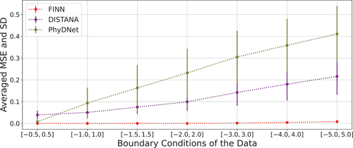
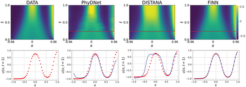
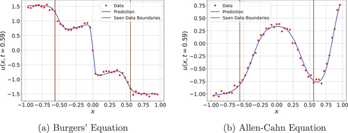
Figure 4. The predictions of the multi-BC trained Allen–Cahn dynamics after inference. First row shows the models’ predictions over space and time. Areas below the red line are the 30 simulation steps that were used for inference and filled with data for visualization. Test error is computed only with the upper area. Second row shows the predictions over $x$ and $u(t=1,x)$, i.e., $u$ in the last simulation step. Data is represented by the red dots and the predictions by the blue line. Best models are used for the plots.

Single-BC Training and Inference

In this experiment, the models receive only one sequence with $t=[0,2]$, $N_t=256$ and $N_x=49$ in training. The BC values of the dataset are constant and set to $[0.0,0.0]$. Hence, the models do not see how the equations behave under different BC values. This is substantially harder compared to the previous experiment, as clearly reflected in the results (see Table 3 and Figure 5). Despite low training errors, DISTANA and PhyDNet fail to infer correct BC values. The prediction errors when testing in closed-loop after BC inference also indicate that these models have difficulties solving the task. Although FINN manages to capture the correct BC values, its prediction error increases significantly when compared to the training error, particularly in the case of Burgers’ equation. Nonetheless, FINN produces the lowest test error by orders of magnitude for both equations. These results demonstrate that FINN significantly benefits from sequences with various BC values, enabling it to infer and predict the same equations over a larger range of novel BCs. Due to space constraints, we only report the results of one set of boundary conditions for each experiment. We observed similar results in experiments with several other BC values.

Figure 5. The predictions of the single-BC trained Burgers’ dynamics after inference. First row shows the models’ predictions over space and time. Areas below the red line are the 30 simulation steps that were used for inference and filled with data for visualization. Test error is computed only with the upper area. Second row shows the predictions over $x$ and $u(x,t=2)$, i.e., $u$ in the last simulation step. Data is represented by the red dots and the predictions by the blue line. Best models are used for the plots.

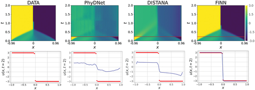
Table 3. Comparison of single-BC training and prediction errors along with the inferred BC values by the corresponding models. The experiments were repeated 5 times for each trial and the average results are presented. Burgers’ dataset BC $=[3.0,-3.0]$ and Allen–Cahn dataset BC $=[-1.0,1.0]$.

Eqn.	Model	Training error	Test error	Inferred BC
Burgers’	DISTANA	$(8.4\pm 1.7)\cdot {10}^{-7}$	$4.14\pm 0.82$	$[-2.5\pm 3.41,+3.0\pm 7.31]$
	PhyDNet	$(1.4\pm 0.9)\cdot {10}^{-4}$	$5.12\pm 0.47$	$[+4.1\pm 3.24,+2.5\pm 8.36]$
	FINN	$(1.7\pm 1.5)\cdot {10}^{-7}$	$0.17\pm 0.16$	$[+3.0\pm 0.01,-3.0\pm 0.01]$
Allen–Cahn	DISTANA	$(1.5\pm 0.4)\cdot {10}^{-5}$	$0.09\pm 0.03$	$[-3.87\pm 3.18,0.12\pm 11.26]$
	PhyDNet	$(4.8\pm 2.2)\cdot {10}^{-5}$	$0.08\pm 0.04$	$[-1.35\pm 1.23,1.92\pm 1.610]$
	FINN	$(2.9\pm 4.2)\cdot {10}^{-6}$	$(1.7\pm 1.4)\cdot {10}^{-5}$	$[-0.99\pm 0.01,0.99\pm 0.006]$

Physical Domain Reconstruction

Our final experiment differs from the previous two in that not only the BCs were inferred, but also a large part of the simulation domain itself. The training process is similar to Section 4.2.1. Ten sequences are created with $t=[0,1]$, $N_t=128$ and $N_x=29$ (compared to 49 earlier). In analogy to Section 4.2.1, we train the models on a variety of different BC values randomly sampled from the same range as before, that is, $[-1,1]$ and $[-0.3,0.3]$ for Burgers’ and Allen–Cahn’s equation, respectively. The inference dataset is generated with $N_x=49$ and the outside-of-training-range BCs are set to $[1.5,-1.5]$ for Burgers’ and $[-1.0,1.0]$ for Allen–Cahn. At inference, the models’ field of view remains restricted to the 29 out of 49 spatial data points. Moreover, the BCs are also unknown to the models. Intuitively, the inference process could correspond to the situation where the models obtain data only from Germany. However, they need to predict the weather not only for Germany but also for the whole of Central Europe. Needless to say that the models need to infer reasonable BC values for the larger domain as well.

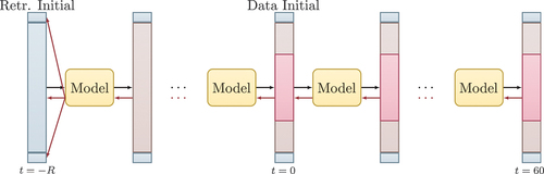
In order to approach this problem, we applied active tuning (AT, Otte, Karlbauer, and Butz 2020). Technically, along with retrospectively inferring unknown values, that is, BCs and unobserved domain sections, AT involves forward passing cycles to incrementally clean its current solution and make it consistent with the model dynamics before generating predictions. The latter can be regarded as a repeatedly applied spin-up phase known from physics simulations. The algorithm and task are visualized in Figure 6.

Figure 6. Active tuning algorithm. $R$ corresponds to the retrospective tuning horizon as stated in Otte, Karlbauer, and Butz (2020). The blue column represents the retrospective initial state and the BCs, which are optimized depending on the gradient-signal. The red areas in the middle of the columns are so-called seen areas from which the models receive information and that provide the error signal. The brown areas are called unseen area and models need to reconstruct the equation, i.e., the $u$ values for the entire domain. Black and red arrows represent the model forward and backward passes, respectively. The gradient information (red arrows) is used to infer the BCs.

As our approach is a gradient-based optimization procedure, the weight updates and error minimization are realized on the basis of the error signal (we apply the mean squared error). However, the error signal does not represent the internal state of the models. That is, a predicted $u_i^t$ and $u_{i+1}^t$ (i.e., two adjacent volumes) can differ meaningfully, but still yield a small error when unrolling the model into the future. Notwithstanding, such large local differences are not a realistic scenario. In fact, FINN’s internal state can provide a measure for such nonrealistic states, as the adjacent volumes are computed with respect to each other in the underlying FVM. Therefore, we optimize and search for an arbitrary solution at $t=-R$ and recruit the model’s simulation output at $t=0$ (starting from $t=-R$) as initial state. A visualization of how the model tunes its predictions in the past is provided in Figure 7 for $R=10$. Although the optimized retrospective initial states at $t=-R$ are ragged, FINN smooths its prediction during the forward pass and thus produces an initial state at $t=0$ that is consistent with the model’s physics and has been cleared from all implausible artifacts. The initial state prediction of all models can be seen in Figure 8 DISTANA and PhyDNet neither manage to predict how the equation would unfold for the seen domain after inference (i.e., time steps between $60-128$), nor can they reconstruct the unseen domain. Figure 8(b) clearly shows how DISTANA can make use of the information it receives as it predicts well inside the seen data boundaries. However, DISTANA is incapable of reconstructing the areas from which it receives no information. We see this as further evidence for the importance of incorporating physical inductive biases, which are not present in DISTANA.

Figure 7. Retrospective state inference. The red lines at $t=0$ show the ground truth, i.e., the initial state of the dataset. The brownish faces indicate the seen area. Best models are used.

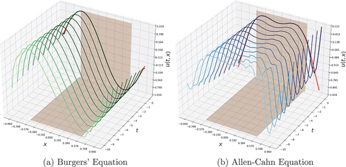
Figure 8. Initial state inference. Figures depict the initial state prediction of the models for $5$ trials. Each light blue line corresponds to one trial. Dataset BC are [1.5, −1.5]. BC-Errors are computed as root mean squared error and are depicted as red lines showing the deviation from the red dots which represent the actual BC values. The plots correspond to the results reported in Table 4.

Table 4. Comparison of seen domain and whole-domain prediction errors along with the inferred BC values by the corresponding models. The experiments were repeated $5$ times for each trial and the average results are presented. Burgers’ dataset BC $=[1.5,-1.5]$ and Allen–Cahn dataset BC $=[-1.0,1.0]$. R = $10$. As 60 data points were used in this experiment (compared to 30 time steps in the previous ones) an error comparison with the other experiments is not possible.

Eqn.	Model	Seen domain error	Whole domain error	Inferred BC
Burgers’	DISTANA	$0.165\pm 0.133$	$0.166\pm 0.136$	$[3.19\pm 0.819,-2.12\pm 0.451]$
	PhyDNet	$0.243\pm 0.056$	$0.715\pm 0.284$	$[0.81\pm 3.415,-0.27\pm 1.314]$
	FINN	$0.006\pm 2\cdot {10}^{-5}$	$0.003\pm 3\cdot {10}^{-5}$	$[1.49\pm 0.008,-1.49\pm 0.003]$
Allen–Cahn	DISTANA	$0.272\pm 0.173$	$0.466\pm 0.422$	$[+1.195\pm 2.76,-1.07\pm 4.02]$
	PhyDNet	$0.517\pm 0.270$	$0.736\pm 0.236$	$[-0.003\pm 0.26,-0.83\pm 1.07]$
	FINN	$(2\pm 0.5)\cdot {10}^{-5}$	$0.013\pm 0.003$	$[-1.038\pm 0.07,+0.67\pm 0.03]$

The quantitative results depicted in Table 4 demonstrate, once again, clear superiority of FINN compared to DISTANA and PhyDNet. The seen domain error corresponds to the error for the time steps after the inference and within the domain from which the models obtained information during inference. The whole domain error, on the other hand, subsumes the seen domain error while also including the reconstruction error from the unseen domain. The larger whole-domain error over the seen domain error of FINN for Burgers’ Equation is likely caused by the high non-linearity of Burgers’ equation in the middle of the spatial domain, compared to more linear dynamics on the edges (c.f. Figure 5). Another interesting point is the inferred BC values of FINN. Despite the significant increase in task complexity and the availability of less data compared to the previous experiments, FINN still achieves accurate BC predictions. However, this is not the case for the right BC in Allen–Cahn. The predicted value stays consistently below the true BC. This might result from arbitrary and nonrealistic BC values chosen for inference data. Furthermore, the BCs contravene with the initial state. As depicted in Figure 7b at $t=0$, the right edge of the data’s initial state (red line) is as low as $-0.91$. The gradients reaching the spatial domain push the prediction to fit the initial state. On the contrary, gradients going to the boundary conditions drive the prediction upward because the right BC is $1$. This is evident in Figure 7b, where the predictions of the right-hand side tend to raise toward the BC. FINN's reaction to this nonrealistic contradiction, however, underlines its strive to find a most plausible and overall consistent explanation. Note that this situation does not occur in the left BC because both the domain and the BC have a higher match.

Physical Domain Reconstruction with Noise

In this section, we tested the performance of the models to reconstruct the missing spatial data and infer unknown boundary conditions from noisy data. The noise robustness of FINN has formerly been demonstrated in Karlbauer et al. (2022). Therefore, the same trained models as in Section 4.3 are used. However, at inference, the models now receive the masked and noisy data.

Data is generated with the same parameters besides that normal-distributed noise with standard deviation $0.05$ is added, following the experimental setup in Karlbauer et al. (2022). Figure 9 gives an idea how strong the noise is in relation to the signal’s magnitude. As it is harder to realize the underlying structure of the equation with noisy data, a longer sequence was needed to make FINN generate meaningful predictions. Thus, we used $80$ time steps instead of $60$ in the previous section. The inference length and data noise are the only differences in the experiment design. The test sequence, i.e., the remaining $42$ time steps from the whole sequence, does not contain any noise.

Figure 9. FINN prediction with noisy data. The red dots show the data and the blue line is the prediction of the model. The area between brown lines indicates the seen area. Best models are used.

The results in Table 5 support the previous indications. FINN’s robust and adaptable architecture allows to extract an accurate structure from noisy data, whereas the other two models fail to generate meaningful predictions. Notwithstanding, noisy data brings its challenges and this can also be seen in FINN’s performance. In particular, the standard deviations of the inferred BCs are relatively high compared to the results in Table 4.

Table 5. Comparison of seen domain and whole-domain prediction errors along with the inferred BC values by the corresponding models inferred on noisy data. The experiments were repeated $5$ times for each trial and the average results are presented. Burgers’ dataset BC $=[1.5,-1.5]$ and Allen–Cahn dataset BC $=[-1.0,1.0]$. R = $10$. As 80 data points were used in this experiment (compared to 30 and 60 time steps in the previous ones) a direct error comparison with the other experiments is not possible.

Eqn.	Model	Seen domain error	Whole domain error	Inferred BC
Burgers’	DISTANA	$0.148\pm 0.080$	$0.160\pm 0.101$	$[4.20\pm 0.919,-3.22\pm 1.480]$
	PhyDNet	$0.259\pm 0.021$	$0.658\pm 0.166$	$[0.45\pm 3.415,-1.83\pm 2.253]$
	FINN	$(9.3\pm 0.3)\cdot {10}^{-3}$	$(5.6\pm 0.2)\cdot {10}^{-3}$	$[1.50\pm 0.016,-1.49\pm 0.010]$
Allen–Cahn	DISTANA	$0.211\pm 0.163$	$0.444\pm 0.428$	$[+0.66\pm 1.414,-0.67\pm 2.621]$
	PhyDNet	$0.603\pm 0.301$	$0.839\pm 0.363$	$[-0.07\pm 0.248,-0.18\pm 0.269]$
	FINN	$(3.94\pm 1.8)\cdot {10}^{-5}$	$0.009\pm 0.011$	$[-0.884\pm 0.44,+0.82\pm 0.141]$

Discussion

The aim of our first experiment (see Section 4.1) was to assess whether FINN, DISTANA, and PhyDNet are able to learn the fixed and unknown Dirichlet BC values of data generated by Burgers’ and Allen–Cahn equations. This was achieved by setting the value of the BC as a learnable parameter to optimize it along with the models’ weights during training. The results, as detailed in Table 1, suggest two conclusions: First, all models can satisfactorily approximate the equations by achieving error rates far below ${10}^{-1}$. Second, only FINN can infer the BC values underlying the data accurately. Although DISTANA and PhyDNet simulate the process with high accuracy, they apparently do not exhibit an explainable and interpretable behavior. Instead, they treat the BC values in a way that does not reflect their true values and physical meaning. This is different in FINN, where the inferred BC values can be extracted and interpreted directly from the model. This is of great value for real-world applications, where data often come with an unknown BC, such as in weather forecasting or traffic forecasting in a restricted simulation domain.

In the second experiment (see Section 4.2), we addressed the question of whether the three models can infer an unknown BC value when they have already been trained on (a set of) known BC values. Technically, this is a traditional test for generalization. The results in Table 2 suggest that both DISTANA and PhyDNet decently learn the effect of the different BC values on the data when being trained on a range of BC values. Once the models are trained on one single BC value only (c.f. Table 3); however, the inferred BC values of DISTANA and PhyDNet are far off the true values. This is different for FINN: although the test error on Burgers’ drops considerably, FINN still determines the underlying BC values in both cases accurately, even when trained on one single BC value only.

In the third experiment (see Section 4.3), we extended the BC inference and examined the ability of the models to simultaneously reconstruct a solid amount of data surrounding the simulation domain. Indeed, Table 4 shows that FINN is able to reconstruct a physical spatial domain while only receiving information from a small domain. In order to achieve this goal, a temporal gradient-based algorithm, Active Tuning (Otte, Karlbauer, and Butz 2020), was applied to optimize domain and BC values in the past. Afterward, these optimized values were employed as initial conditions such that the model could tune its prediction solely depending on its own internal dynamics. With this method, FINN reaches a smooth initial state on the basis of which it starts its prediction at $t=0$ (see Figures 7 and 8). A key advantage of FINN compared to DISTANA and PhyDNet is recognized in the physical knowledge it has about the equations (i.e., Burgers’ and Allen–Cahn). In the last experiment (see Section 4.4, we created a more challenging task and added noise to the data. We used essentially the same experimental design (except for longer inference sequences) and showed FINNs’ robustness in noisy-data regimes.

Our main aim was to infer physically plausible, interpretable BC values and reconstruct a spatial domain. Although FINN is a well-tested model and has been compared with several models such as ConvLSTM, TCN, and CNN-NODE in Karlbauer et al. (2022), we applied FINN to 1D equations in this work only. However, since the same principles underlie in higher dimensional equations, we anticipate the applicability of the proposed method to higher dimensional problems and leave it as an interesting topic for future research.

Conclusion

In a series of experiments, we found that the physics-aware finite volume neural network (FINN) is the only model – among DISTANA (a pure spatiotemporal processing ML approach) and PhyDNet (another physics-aware model) – that can determine an unknown boundary condition value of data generated by two different PDEs with high accuracy. While finding the correct BC values, FINN can also deal with missing data and reproduce around $40\mathrm{\%}$ of the spatial domain. So far, the universal pure ML models stay too general to solve the problem studied in this work. State-of-the-art physics-aware networks, e.g., in Le Guen and Thome (2020) or Em Karniadakis et al. (2021) are likewise not specific enough. Instead, this work suggests that a physically structured model, which can be considered as an application-specific inductive bias, is indispensable and should be paired with the learning abilities of neural networks. FINN integrates these two aspects by implementing multiple feedforward modules and mathematically composing them to satisfy physical constraints. This structure allows FINN to determine unknown boundary condition values both during training and inference, which, to the best of our knowledge, is a unique property among physics-aware ML models. Besides, setting BC values in the form of hyper-parameters on real-world data is an undesirable situation for researchers. Therefore, we interpret this latest component as valuable contribution to the spatiotemporal modeling scene. Moreover, FINN offers explanations of the modeled process, including BC and substance properties, which need to be explored in further detail.

In future work, we will investigate how different BC types (Dirichlet, periodic, Neumann, etc.) – and not only their values – can be inferred from data. Moreover, an adaptive and online inference scheme that can deal with dynamically changing BC types and values is an exciting direction to further advance the applicability of FINN to real-world problems. Our long-term aim is to apply FINN to a variety of real-world scenarios of a larger scale, such as to local weather forecasting tasks, and to extend previous work by Praditia et al. (2022). We expect that FINN will be able to generate complete model simulations from sparse data and potentially unknown BCs.

Acknowledgement

This work was partially funded by the Deutsche Forschungsgemeinschaft [EXC 2075 – 390740016] and [EXC 2064 – 390727645]. We acknowledge the support provided by the Stuttgart Center for Simulation Science (SimTech). Matthias Karlbauer was supported by the International Max Planck Research School for Intelligent Systems and the Deutscher Akademischer Austauschdienst. Sebastian Otte was supported by a Feodor Lynen fellowship from the Alexander von Humboldt-Stiftung.

Disclosure statement

No potential conflict of interest was reported by the author(s).

References

- Battaglia, P. W., J. B. Hamrick, V. Bapst, A. Sanchez-Gonzalez, V. Zambaldi, M. Malinowski, A. Tacchetti, D. Raposo, A. Santoro, R. Faulkner, et al. 2018. Relational inductive biases, deep learning, and graph networks. arXiv preprint arXiv:1806.01261.
- Butz, M. V., D. Bilkey, D. Humaidan, A. Knott, and S. Otte. 2019. Learning, planning, and control in a monolithic neural event inference architecture. Neural Networks 117:135–1375. doi:10.1016/j.neunet.2019.05.001.
- Can Horuz, C., M. Karlbauer, T. Praditia, M. V. Butz, S. Oladyshkin, W. Nowak, and S. Otte. 2022. Inferring boundary conditions in finite volume neural networks. In International Conference on Artificial Neural Networks (ICANN), Bristol, United Kingdom, 538–49. Springer Nature Switzerland. doi:978-3-031-15919-0.
- Chen, R. T. Q., R. Yulia, J. Bettencourt, and D. Duvenaud. 2018. Neural ordinary differential equations. Proceedings of the 32nd International Conference on Neural Information Processing Systems. Red Hook, NY, USA. Curran Associates Inc., 6572–6583.
- Em Karniadakis, G., I. G. Kevrekidis, L. Lu, P. Perdikaris, S. Wang, and L. Yang. 2021. Physics-informed machine learning. Nature Reviews Physics 3 (6):422–440. doi:10.1038/s42254-021-00314-5.
- Fletcher, C. A. 1983. Generating exact solutions of the two-dimensional burgers’ equations. International Journal for Numerical Methods in Fluids 3 (3):213–216. doi:10.1002/fld.1650030302.
- Hochreiter, S., and J. Schmidhuber. 1997. Long short-term memory. Neural Computation 9 (8):1735–1780. doi:10.1162/neco.1997.9.8.1735.
- Karlbauer, M., T. Menge, S. Otte, H. P. A. Lensch, T. Scholten, V. Wulfmeyer, and M. V. Butz. 2021. Latent state inference in a spatiotemporal generative model. In International Conference on Artificial Neural Networks (ICANN), Bratislava, Slovakia, 384–95. Springer International Publishing. doi:978-3-030-86380-7.
- Karlbauer, M., S. Otte, H. P. A. Lensch, T. Scholten, V. Wulfmeyer, and M. V. Butz. 2020 October. A distributed neural network architecture for robust non-linear spatio-temporal prediction. In 28th European Symposium on Artificial Neural Networks (ESANN), 303–08, Bruges, Belgium.
- Karlbauer, M., T. Praditia, S. Otte, S. Oladyshkin, W. Nowak, and M. V. Butz. 2022. Composing partial differential equations with physics-aware neural networks. In International Conference on Machine Learning (ICML), Baltimore, USA.
- Le Guen, V., and N. Thome. 2020. Disentangling physical dynamics from unknown factors for unsupervised video prediction. In Proceedings of the IEEE/CVF Conference on Computer Vision and Pattern Recognition, 11474–84.
- Li, Z., N. Kovachki, K. Azizzadenesheli, B. Liu, K. Bhattacharya, A. Stuart, and A. Anandkumar. 2020. Fourier neural operator for parametric partial differential equations. arXiv preprint arXiv:2010.08895.
- Long, Z., Y. Lu, X. Ma, and B. Dong. 2018. Pde-net: Learning PDEs from data. In International Conference on Machine Learning, Stockholm, Sweden, 3208–16. PMLR.
- Moukalled, F., L. Mangani, and M. Darwish. 2016. The Finite Volume Method In Computational Fluid Dynamics : An Advanced Introduction With OpenFOAM and Matlab. In Fluid Mechanics and Its Applications, vol. 113. Cham: Springer International Publishing. doi:10.1007/978-3-319-16874-6.
- Naugolnykh, K. A., L. Ostrovsky, O. A. Sapozhnikov, and M. F. Hamilton. 2000. Nonlinear wave processes in acoustics. The Journal of the Acoustical Society of America 108 (1):14–15. doi:10.1121/1.429483.
- Otte, S., M. Karlbauer, and M. V. Butz. 2020. Active tuning. arXiv preprint arXiv:2010.03958.
- Praditia, T., M. Karlbauer, S. Otte, S. Oladyshkin, M. V. Butz, and W. Nowak. 2021. Finite volume neural network: Modeling subsurface contaminant transport. In International Conference on Learning Representations (ICRL) – Workshop Deep Learning for Simulation.
- Praditia, T., M. Karlbauer, S. Otte, S. Oladyshkin, M. V. Butz, and W. Nowak. 2022. Learning groundwater contaminant diffusion-sorption processes with a finite volume neural network. Water Resources Research 58 (12). doi:10.1029/2022WR033149.
- Raissi, M., P. Perdikaris, and G. E. Karniadakis. 2019. Physics-informed neural networks: A deep learning framework for solving forward and inverse problems involving nonlinear partial differential equations. Journal of Computational Physics 378:686–707. doi:10.1016/j.jcp.2018.10.045.
- Sculley, D., G. Holt, D. Golovin, E. Davydov, T. Phillips, D. Ebner, V. Chaudhary, M. Young, J.F. Crespo, and D. Dennison. 2015. Hidden technical debt in machine learning systems. In Proceedings of the 28th International Conference on Neural Information Processing Systems 2(15): 2503–11, Cambridge, MA, USA: MIT Press.
- Seo, S., C. Meng, and Y. Liu. 2019. Physics-aware difference graph networks for sparsely-observed dynamics. In International Conference on Learning Representations, New Orleans, USA.
- Sitzmann, V., J. Martel, A. Bergman, D. Lindell, and G. Wetzstein. 2020. Implicit neural representations with periodic activation functions. Advances in Neural Information Processing Systems 33:7462–7473.
- Yin, Y., V. Le Guen, J. Dona, E. de Bézenac, I. Ayed, N. Thome, and P. Gallinari. 2021. Augmenting physical models with deep networks for complex dynamics forecasting. Journal of Statistical Mechanics: Theory and Experiment 20210 (12):124012. doi:10.1088/1742-5468/ac3ae5.