Waveforms Eavesdropping Prevention Framework: The Case of Classification of EPG Waveforms of Aphid Utilizing Wavelet Kernel Extreme Learning Machine

ABSTRACT

Since all information depends solely on the training data, machine learning algorithms typically do not employ external knowledge or other experiences during the learning process. Methods for machine learning have been rigorously tested against novel varieties of highly technical “black box” or “white box” adversarial attacks. By employing attacks, attackers can change systems to serve a harmful end goal. When authorized implementers and eavesdroppers are geographically close together, it is difficult to perform secure beamforming in waveform applications, for instance, leading to erroneous beam forms and, as a result, disastrous beam leakages. As a result, the first move in a prospective black-box offense will be based on the waveform features of a learning signal. By including a non-orthogonality concept into the physical layer signal waveform, the Waveforms Eavesdropping Prevention Framework (WEPF) proposed in this work aims to boost machine learning security to address these difficulties. The implementation scenario is based on a waveforms scenario used to categorize the Electrical Penetration Graph (EPG) for insects, a crucial tool for researching the feeding conduct of piercing-sucking insects and the transition mechanism between viruses and insects. An attribute vector with six dimensions, consisting of low-frequency wavelet energy (LFWE) in the second and third layers of the Wavelet Kernel Extreme Learning Machine, fractal box dimension (FBD), the Hurst exponent (HE), and spectral centroid (SC) in the first two layers of the HHT, was used to test the proposed framework. Two adversarial scenarios were explored. However, the suggested architecture secures all waveform signals, demonstrating the method’s effectiveness in lowering the risk of eavesdropping or tampering with the waveforms used in advanced machine-learning methods.

Introduction

Machine learning has become an increasingly important technology in many fields, including computer vision, natural language processing, robotics, and autonomous systems. However, machine learning algorithms are vulnerable to adversarial attacks, which can lead to incorrect or even malicious decisions with serious consequences. Adversaries can manipulate the input data or the learning process to exploit vulnerabilities in the algorithm and achieve their goals. Therefore, improving the security of machine learning algorithms is a critical research area.

One of the challenges in securing machine learning algorithms is that they typically rely solely on the training data to acquire knowledge and make decisions. However, this approach can be vulnerable to attacks that manipulate the training data or exploit biases in the data distribution. Therefore, it is essential to incorporate additional knowledge or experience into the learning process to improve the algorithm’s robustness and security.

Using specialized computational models and automation systems built on cutting-edge technical infrastructure is necessary for the management of modern science in general, as well as for the supervision and optimization of its operations. To achieve complete automation, higher-level communications and information technology solutions are required, including seamless networking and technologies for intelligent data analysis. Still, this reality raises serious concerns about the dependability of the technical processes being utilized, particularly those concerned with digital threats that can be physically and conceptually exploited. The question technologies bring with them a landscape of digital risks and cyberattacks, which results in establishing a new regulatory system that is extremely vulnerable. Intelligent systems, despite being able to demonstrate logic, experiential learning, and the ability to make optimal decisions without human intervention, bring extra security challenges throughout the full length of their implementation line. These security issues include the possibility of an adversary manipulating the training data to take advantage of the model’s sensitivity and impact its performance in a way that benefits the attacker. In particular, the training and testing phases determine the threats’ various grades and degrees of intensity.

The targets of machine learning assaults can be determined in several ways, including by using the physical domain, input sensors, digital representation for preprocessing operations, the algorithm itself, or the physical domain of output activities. It is believed that supervised learning systems, widely utilized in many intelligent applications that use waveforms, are the most vulnerable type of machine learning system, even though all types of machine learning systems are, in theory, vulnerable to attack.

The following are some of the characteristics of machine learning algorithms that contribute to the development of artificial intelligence but also make systems more vulnerable to assault:

1. Characteristic 1: The process of machine learning results in forming fairly fragile patterns that are effective but readily derailed. The statistical associations that machine learning models develop are typically quite fragile and readily broken. Attackers can take advantage of this vulnerability by initiating assaults, which results in a model that is otherwise superb performing below expectations.

2. The most common reason a machine learning model is unsuccessful is when it places too much weight on the data alone. The system is harmed due to possible data poisoning, and it becomes easier for malicious actors to carry out their malicious operations. Only through collecting patterns from data sets can machine learning models be taught and learned. The problematic models do not have the essential parallel knowledge that would enable them to utilize all of the information; as a result, their comprehension is wholly reliant on the data with which they are trained.

3. Characteristic 3: The inability to correctly comprehend modern machine learning algorithms makes it difficult to exercise control over them (black box algorithms). Deep neural networks, for example, are among the most cutting-edge approaches based on machine learning; despite their widespread use, these methods are still considered black-box algorithms in many respects because it is fundamentally difficult to grasp them fully. Because of this, it is extremely difficult, if not impossible, to determine whether a machine learning algorithm has been hacked, is being attacked, or is simply not doing as well as it should be.

These flaws explain why no ideal repair strategies can be implemented when AI attacks are carried out. They also explain why the attacks are very different from the typical cybersecurity challenges, in which vulnerabilities are clearly defined even if it is difficult to uncover them.

The first step on the path toward a potential black-box attack will be learning the properties of the signal waveform. Rosaries could use these attacks to deceive systems into changing behavior to accomplish a potentially destructive end goal. For instance, secure beamforming presents several difficulties in waveform applications when authorized users and eavesdroppers are close to one another. This is because imprecise beam forms and, as a result, damaging beam leakages make the task difficult.

The context and issues surrounding the need for secure machine learning algorithms can be exposed as follows:

1. Adversarial attacks in machine learning: Machine learning algorithms are vulnerable to adversarial attacks, where attackers can change systems to serve a harmful end goal. These attacks have been rigorously tested against various technical “black box” or “white box” adversarial attacks, making it crucial to enhance the security of machine learning algorithms.

2. Difficulty in secure beamforming: When authorized implementers and eavesdroppers are geographically close together, it becomes difficult to perform secure beamforming in waveform applications, leading to erroneous beam forms and beam leakages.

3. Importance of waveform signals in machine learning: Waveform signals are an essential component of advanced machine learning methods and their tampering or eavesdropping can result in disastrous consequences.

These are the context and issues that the WEPF aims to address. By incorporating non-orthogonality into the physical layer signal waveform, the WEPF aims to enhance the security of machine learning algorithms, especially in scenarios where authorized implementers and eavesdroppers are close to each other.

To carry out exhaustive research on how to defend against adversarial attacks against waveforms, it is necessary to have both a respectable sentence. Within this environment, exhaustive experiments will be carried out, and the results of these experiments will be used to evaluate any process (Xu 2020, 2021).

Scenario

Most types of Aphids, which are characterized as tiny plant piercing-sucking insects (PSIs), are significant pests used for both agriculture and forestry such as Aphis gossypii (AG), Myzus persicae (MP), Aphis glycines (AR), and Rhopalosiphum padi (RP). Besides, they are called the most significant vectors on which plant viruses exist.

A powerful device, called the insect electrical penetration graph (EPG), was utilized to examine the nourishing conduct of PSIs (Jallingii 1978; Tjallingii 1985, 2014), both insect transmission and crop resistance mechanisms, etc. Thus, its technical capability could help prevent and control piercing-sucking insects. More than 50 insects are studied successfully with this device so far. Some most widely studied ones are called aphids, whiteflies, planthoppers, leafhoppers, thrips, and bugs.

Once the implementation of the EPG is under consideration for the investigation of both insects and plants, correct classification of EPG waveforms is required. Manual processes have been employed so far. Thus, analyzing EPG signals and extracting insights lead to obtaining statistics by employing software such as Stylet, Probing, and Statistical Analysis Systems programming (Ebert et al. 2015). However, the classification of waveforms still needs to be operated manually even though the latest version of the mentioned software is in use before statistical analysis is run.

The literature has two research related to grouping waveforms of EPG for Aphid. A method called the assisted examination of EPG abbreviated as A2EPG was suggested to analyze the EPG waveform by Adasme-Carreño et al. (2015). Thus, the waves such as np, C, pd, G, and E1 are identified and the time in every band is measured. Nevertheless, A2EPG does not generate a better accuracy ratio. While waves of np and pd are recognized very well, waves of E2 and F could not be identified. On the other hand, G and E1 waves are misdeemed as C waves. Thus, reexamination of outcomes should be conducted when outcomes are obtained.

The method used to extract and recognize attributes is so immature that the A2EPG gives a lower recognition ratio. Other issues are expressed as follows: while the extreme and slope attributes of the waveform related to the time domain are extracted, both time-frequency and non-linear attributes are not considered. While the computational complexity to a certain extent is reduced by this method, the general attributes of the waveform are represented partially, which results in ignoring significant details in the waveforms. Moreover, the binary classifier, poorer in learning by itself and non-linear data crunching than machine learning methods, is employed by A2EPG.

The EPG signals emitted by aphids are researched to extract attributes and classify the waves of np, C, E1, E2, and F by Wu et al. (2018). An attribute extraction algorithm that combines both FD and HHT is suggested. Then, a classifier called a decision tree (DT) is utilized. Four grouped samples tested gives a mean recognition ratio of 91.43%. When the comparison is made with the manual method concerning duration, the recognition duration by machine is just 1/46 of the manually conducted one. Thus, the efficacy of the analysis is enormously enhanced.

The research presented by (Wu et al. 2018) discussed preliminaries to extract non-linear attributes and mention classifiers related to decision tree-based methods. Other attributes such as time-frequency ones were not regarded, and other methods related to classification schemes using machine learning were not debated.

As described above, signal analysis methods are exciting and can support cutting-edge systems containing artificial intelligence methods to advance science and the common good. But these methods have been thoroughly sensitive to contemporary types of cyber-attacks. The plans can be manipulated by adversaries employing these offenses to alter the system into a malicious end objective. When the further integration of AI-based systems into delicate science constituents is realized, these offenses pose an emerging and systemic sensitivity that potentially has significant implications for global security. It should be said that there exist fundamental differences between conventional cyber-attacks and new types, which are certainly different from ones related to bugs or human errors in the scripts. Inherent constraints embedded in AI methods that cannot be remedied or are very tough to fix could lead to AI attacks. More generally, the methods used for functioning AI systems efficiently are flawed, and adversaries utilize those constraints embedded in the systems to attack.

Furthermore, the set of entities utilized by AI offenses is expanded to realize cyber-attacks. They start with utilizing physical objects first. Then, manipulation of data in new ways is employed. When it occurs, how information is collected, placed, and utilized is changed to prevent potential exploitation.

Therefore, this manuscript proposes the WEPF, attempting to increase machine learning security by including a non-orthogonality idea into the physical layer signal waveform. Also, various attribute derivation methodologies and classification methods are utilized to study the better clustering of EPG waveforms.

The sections of the manuscript are constructed subsequently. Section 2 presents the common waveforms utilized in the signal analysis of the EPG. The presentation of the extreme kernel learning machine is presented in Section 3. Section 4 is allocated to present the feature extraction, the proposed method, and its implementation. Section 5 concludes the research.

The Common Waveforms Employed in the Analysis of EPG Signals

The EPG signals carry biological importance for the behavior of PSIs. Those are pertinent to both plant and insect species and vary widely in all types, namely, aphids, leafhoppers, lygus lucorum, etc.

The signal of the EPG is used to study the piercing-sucking characteristics of Aphids, which is the first insect. The EPG waveforms have been researched most comprehensively. Eight fundamental waveforms and their importance related to biological attributes have been documented clearly (Alba-Tercedor, Hunter, and Alba-Alejandre 2021; Backus, Shih, and Weintraub 2020; Cornara et al. 2018; Jing, Bai, and Liu 2013; Prado and Tjallingii 1994; Tjallingii and Esch 1993). np, A, B, C, pd, E, G, and F waves are the eight of the waveforms. A non-penetration wave is denoted by np whose waveform is represented by an almost straight line, which implies that the plant epidermis cannot be penetrated by aphid stylets. The path waves are denoted by A, B, and C, respectively. The water-soluble saliva secretion always accompanies A. B comes out after A when there exists a secretion of gelatinous saliva, and the aphid stylet (AS) is situated at the epidermis and parenchyma. C comes out following B. No definite line exists between them. The most complicated is the C wave. When the analysis of EPG waves is conducted, namely, the AS is situated between the epidermis and the microtubule bundle. Once the identification of the waveforms is realized, some of them not separated are mainly grouped as C. Both A and B waves were also statistically grouped as C waves. The mouth needle designates the puncture wave denoted by pd. Thus, when the cell membrane is punctured by an aphid, it measures the possible disparity between the inside and outside of the membrane. The operating syringe located at the mouth exploring the sieve tube in the phloem is characterized by E, which is categorized into two waves called El (the phloem secretes saliva wave and E2 (the phloem-feeding wave). While a xylem feeding wave is denoted by G, a mechanical barrier wave is characterized by F. Figure 1 depicts the characteristic waveforms of the EPG. So, the handbook of the EPG system can be employed as a source sample to interpret many waveforms.

Figure 1. The EPG waveforms of aphid feeding.

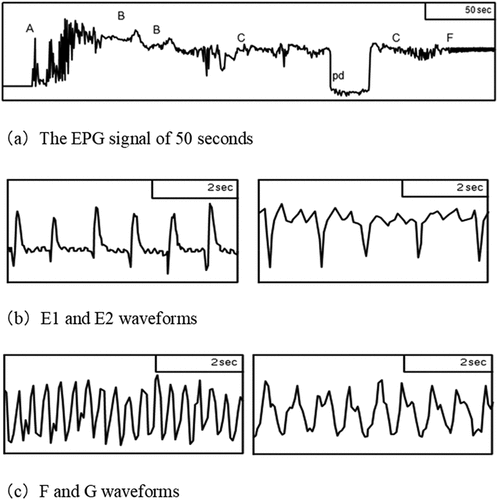
When the nourishing conduct of insects, plant resistance system, or mechanism of virus transmission is examined by EPG, manual identification of the aforementioned waveforms is generally required. Afterward, the parameters of each waveform are analyzed.

Wavelet Kernel Extreme Learning Machine

Huang et al. advanced a single hidden layer feedforward neural network (SLFN) utilizing Extreme Learning Machine (ELM) to overcome the issues of conventional NNs whose training speed is slow, and it easily falls into the local smallest score. The weights between the input and hidden layers and the threshold for the hidden layer neuron are produced randomly in the ELM. Assigning the neuron numbers within the hidden layer during the training operation leads to the optimum outcome. When the comparison is made with the conventional SLFN, both faster learning speed and better performance for generalizability appear to be the advantages. Hence, it has been extensively employed in analyses such as regression, data fitting, and classification detection (Huang 2015).

Figure 2 depicts the network edifice of the ELM, which is composed of input, hidden, and output layers. All neurons in this network are fully connected with no exception as depicted.

Figure 2. The network edifice of the ELM.

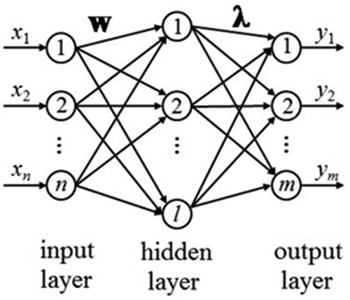
Suppose that the input layer consisting of n neurons corresponds to n input attributes. While l neurons are contained in the hidden layer, m neurons are included in the output layer that corresponds to m output attributes. The matrix representing connection weights between the input and the hidden layers is denoted by$\mathit{w}$. The matrix representing relation weights between the hidden and the output layers is represented by $\mathit{\lambda }$. The matrix representing the threshold of the hidden layer neurons is represented by $\mathit{b}$, then

(1) $\mathbf{w}=\left[\begin{array}{c}{w}_1\\ w_2\\ ⋮\\ w_l\end{array}\right]={\left[\begin{array}{c}\begin{array}{cccc}{w}_{11}& w_{12}& \cdots & w_{1n}\end{array}\\ \begin{array}{cccc}{w}_{21}& w_{22}& \cdots & w_{2n}\end{array}\\ \begin{array}{cccc}⋮& ⋮& \cdots & ⋮\end{array}\\ \begin{array}{cccc}{w}_{l1}& w_{l2}& \cdots & w_{ln}\end{array}\end{array}\right]}_{l\times n}$(1)

(2) $\lambda =\left[\begin{array}{c}{\lambda }_1\\ {\lambda }_2\\ ⋮\\ {\lambda }_l\end{array}\right]={\left[\begin{array}{c}\begin{array}{cccc}{\lambda }_{11}& {\lambda }_{12}& \cdots & {\lambda }_{1m}\end{array}\\ \begin{array}{cccc}{\lambda }_{21}& {\lambda }_{22}& \cdots & {\lambda }_{2m}\end{array}\\ \begin{array}{cccc}{\hspace{0.17em}}_{\hspace{0.17em}}^{\hspace{0.17em}}⋮& {\hspace{0.17em}}_{\hspace{0.17em}}^{\hspace{0.17em}}{\hspace{0.17em}}_{\hspace{0.17em}}^{\hspace{0.17em}}⋮& {\hspace{0.17em}}_{\hspace{0.17em}}^{\hspace{0.17em}}\cdots & {\hspace{0.17em}}_{\hspace{0.17em}}^{\hspace{0.17em}}⋮\end{array}\\ \begin{array}{cccc}{\lambda }_{l1}& {\lambda }_{l2}& \cdots & {\lambda }_{lm}\end{array}\end{array}\right]}_{l\text{timesm}}$(2)

(3) $\mathit{b}={\left[\begin{array}{c}{b}_1\\ b_2\\ ⋮\\ b_l\end{array}\right]}_{l\times 1}$(3)

If $G\left(x\right)$is assigned as the activation mapping for the input layer, $\mathit{Y}$denotes the outcome of the network

(4) $\mathit{Y}=\mathit{H}\mathit{\lambda }$(4)

where $\mathit{H}$ and N represents the output matrix for the hidden layer and the output data number, respectively.

(5) $H=\left[\begin{array}{cccc}G\left(w_1\cdot x_1+b_1\right)& G\left(w_2\cdot x_1+b_2\right)& \cdots & G\left(w_L\cdot x_1+b_L\right)\\ G\left(w_1\cdot x_2+b_1\right)& G\left(w_2\cdot x_2+b_2\right)& \cdots & G\left(w_L\cdot x_2+b_L\right)\\ ⋮& ⋮& ⋮& ⋮\\ G\left(w_1\cdot x_N+b_1\right)& G\left(w_2\cdot x_N+b_2\right)& \cdots & G\left(w_L\cdot x_N+b_L\right)\end{array}\right]={\left[\begin{array}{c}h\left(x_1\right)\\ h\left(x_2\right)\\ \text{amp}⋮\\ h\left(x_N\right)\end{array}\right]}_{N\times L}$(5)

The equation represents a neural network with an input, hidden, and output layer. The input layer is represented by the variables $x_1$ through $x_N$, the hidden layer is represented by the function $h\left(x\right)$, and the output layer is represented by the matrix $H$.

Huang suggests two theorems related to the convergence of the ELM algorithm. The first theorem states that if the hidden layer of the ELM has the same number of neurons as the training set has data points for each weight and bias value, the ELM can converge to the training set with zero error. The second theorem states that if the training set has a large number of data points, the ELM can converge to an acceptable training error (ε >0) by using a hidden layer with fewer neurons than the number of data points, to reduce the computational complexity of the algorithm.

The statement “the ELM can converge to an acceptable training error (ε >0)” suggests that the ELM algorithm can achieve a training error that is greater than zero but still small enough to be considered acceptable. A training error of ε = 0.1 might be acceptable, while a smaller error of ε = 0.01 might be required in others. The acceptable training error depends on the complexity of the model and the amount of available data for training.

Thus, as $G\left(x\right)$, the mapping for activation, has the property of being infinitely differentiable, the whole parameters are not needed to be tuned. Both $\mathit{w}$ and $\mathit{b}$ parameters could be picked randomly before the training stage is conducted and are kept fixed when training is in progress. The affinity weights $\mathit{\lambda }$ between the hidden and the output layers are attained by the LS result represented in Equation 33(32) $Untargeted:\mathrm{m}\mathrm{i}{\mathrm{n}}_{\mathrm{x}{ }^{\mathrm{\prime }}}\mathrm{d}\left(\mathrm{x}{ }^{\mathrm{\prime }},\mathrm{x}\right)\mathrm{s}\mathrm{u}\mathrm{b}\mathrm{j}\mathrm{e}\mathrm{c}\mathrm{t}\mathrm{t}\mathrm{o}\mathrm{C}\left(\mathrm{x}{ }^{\mathrm{\prime }}\right)\ne \mathrm{C}\left(\mathrm{x}\right)$(32) .

(6) $\underset{\lambda }{min}||H\lambda -Y||$(6)

The solution is represented by

(7) $\hat{\mathit{\lambda }}={\mathit{H}}^{+}\mathit{Y}$(7)

where ${\mathit{H}}^{+}$denotes the generalized Moore-Penrose inversion of the output matrix of the hidden layer $\mathit{H}$.

Equation 33(32) $Untargeted:\mathrm{m}\mathrm{i}{\mathrm{n}}_{\mathrm{x}{ }^{\mathrm{\prime }}}\mathrm{d}\left(\mathrm{x}{ }^{\mathrm{\prime }},\mathrm{x}\right)\mathrm{s}\mathrm{u}\mathrm{b}\mathrm{j}\mathrm{e}\mathrm{c}\mathrm{t}\mathrm{t}\mathrm{o}\mathrm{C}\left(\mathrm{x}{ }^{\mathrm{\prime }}\right)\ne \mathrm{C}\left(\mathrm{x}\right)$(32) presents the solution

(8) $\hat{\mathit{\lambda }}={\mathit{H}}^T(\mathit{H}{\mathit{H}}^T+\frac{I}{C}{)}^{-1}\mathit{Y}$(8)

where C represents a tunable parameter.

Equation 33(32) $Untargeted:\mathrm{m}\mathrm{i}{\mathrm{n}}_{\mathrm{x}{ }^{\mathrm{\prime }}}\mathrm{d}\left(\mathrm{x}{ }^{\mathrm{\prime }},\mathrm{x}\right)\mathrm{s}\mathrm{u}\mathrm{b}\mathrm{j}\mathrm{e}\mathrm{c}\mathrm{t}\mathrm{t}\mathrm{o}\mathrm{C}\left(\mathrm{x}{ }^{\mathrm{\prime }}\right)\ne \mathrm{C}\left(\mathrm{x}\right)$(32) denotes the result of the classifier called ELM.

(9) $f\left(\mathit{x}\right)=h\left(\mathit{x}\right){\mathit{H}}^T(\mathit{H}{\mathit{H}}^T+\frac{I}{C}{)}^{-1}\mathit{Y}$(9)

The result of the hidden layer of each sample is considered an attribute map of the sample in the ELM. Equation 33(32) $Untargeted:\mathrm{m}\mathrm{i}{\mathrm{n}}_{\mathrm{x}{ }^{\mathrm{\prime }}}\mathrm{d}\left(\mathrm{x}{ }^{\mathrm{\prime }},\mathrm{x}\right)\mathrm{s}\mathrm{u}\mathrm{b}\mathrm{j}\mathrm{e}\mathrm{c}\mathrm{t}\mathrm{t}\mathrm{o}\mathrm{C}\left(\mathrm{x}{ }^{\mathrm{\prime }}\right)\ne \mathrm{C}\left(\mathrm{x}\right)$(32) represents this attribute map substituted by a kernel mapping proposed by (Diker et al. 2019).

$\mathit{H}{\mathit{H}}^T\left(i,j\right)=K\left(x_i,x_j\right)$

(10) $\mathit{H}{\mathit{H}}^T={\mathrm{\Omega }}_{ELM}=\left[\begin{array}{ccc}K\left(x_1,x_1\right)& \cdots & K\left(x_1,x_N\right)\\ ⋮& ⋮& ⋮\\ K\left(x_N,x_1\right)& \cdots & K\left(x_N,x_N\right)\end{array}\right]$(10)

$h\left(\mathit{x}\right){\mathit{H}}^T=\left[\begin{array}{c}K\left(x_1,x_1\right)\\ \begin{array}{cc}& ⋮\end{array}\\ K\left(x_1,x_N\right)\end{array}\right].$

The result of the ELM classifier alters through Equation 33(32) $Untargeted:\mathrm{m}\mathrm{i}{\mathrm{n}}_{\mathrm{x}{ }^{\mathrm{\prime }}}\mathrm{d}\left(\mathrm{x}{ }^{\mathrm{\prime }},\mathrm{x}\right)\mathrm{s}\mathrm{u}\mathrm{b}\mathrm{j}\mathrm{e}\mathrm{c}\mathrm{t}\mathrm{t}\mathrm{o}\mathrm{C}\left(\mathrm{x}{ }^{\mathrm{\prime }}\right)\ne \mathrm{C}\left(\mathrm{x}\right)$(32) and Equation 33(32) $Untargeted:\mathrm{m}\mathrm{i}{\mathrm{n}}_{\mathrm{x}{ }^{\mathrm{\prime }}}\mathrm{d}\left(\mathrm{x}{ }^{\mathrm{\prime }},\mathrm{x}\right)\mathrm{s}\mathrm{u}\mathrm{b}\mathrm{j}\mathrm{e}\mathrm{c}\mathrm{t}\mathrm{t}\mathrm{o}\mathrm{C}\left(\mathrm{x}{ }^{\mathrm{\prime }}\right)\ne \mathrm{C}\left(\mathrm{x}\right)$(32) .

(11) $f\left(\mathit{x}\right)={\left[\begin{array}{c}K\left(x_1,x_1\right)\\ \begin{array}{cc}& ⋮\end{array}\\ K\left(x_1,x_N\right)\end{array}\right]}^T({\mathrm{\Omega }}_{ELM}+\frac{I}{C}{)}^{-1}\mathit{Y}$(11)

Where the kernel function is denoted by K. When the wavelet function is utilized by the kernel function, ELM turns out to be called WKELM (wavelet kernel extreme learning machine). The manuscript utilizes the basis of the Morlet wavelet to establish the wavelet kernel mapping. Equation 33(32) $Untargeted:\mathrm{m}\mathrm{i}{\mathrm{n}}_{\mathrm{x}{ }^{\mathrm{\prime }}}\mathrm{d}\left(\mathrm{x}{ }^{\mathrm{\prime }},\mathrm{x}\right)\mathrm{s}\mathrm{u}\mathrm{b}\mathrm{j}\mathrm{e}\mathrm{c}\mathrm{t}\mathrm{t}\mathrm{o}\mathrm{C}\left(\mathrm{x}{ }^{\mathrm{\prime }}\right)\ne \mathrm{C}\left(\mathrm{x}\right)$(32) presents.

(12) $K\left(x_i,x_j\right)=\prod _{i=1}^n\left[cos(1.75\left(\frac{x_i-x_j}{a}\right)\right)exp(-\frac{{(x_i-x_j)}^2}{2a^2})]$(12)

Proposed WEPF

The proposed WEPF is based on an index-modulated nonorthogonal spectrally efficient frequency-division multiplexing (SEFDM) framework in which non-orthogonal subcarriers are index-modulated to reduce the impacts of destructive intercarrier interference while using the SEFDM-specific higher bandwidth efficiency. Furthermore, the model employs a low-complexity successive finding technique utilizing the smallest mean-squared error (MMSE) statistics and Log-Likelihood Ratio-based index modulation finding, allowing us to run the suggested system in a situation with a realistically large number of subcarriers.

In the proposed system, $N$ subcarriers were separated into $L$ classes, each of which contains $M$ subcarriers; hence, $N=LM$. The transmission frame of the whole frequency-domain $\mathrm{s}\in {\mathbb{C}}^N$ is defined by

(13) $\begin{array}{c}s={\left[s_0,s_1,\cdots ,s_{N-1}\right]}^T={\left[{\mathbf{s}}^{\left(0\right)T},{\mathbf{s}}^{\left(1\right)T},\cdots ,{\mathbf{s}}^{\left(L-1\right)T}\right]}^T\\ \hspace{0.17em}\end{array}$(13)

The symbols of the frequency domain in the $l$th subcarrier class are defined by

(14) ${\mathbf{s}}^{\left(l\right)}={\left[s_0^{\left(l\right)},s_1^{\left(l\right)},\cdots ,s_{M-1}^{\left(l\right)}\right]}^T\in {\mathbb{C}}^M$(14)

Also, the signal representation of the time-domain of the suggested framework, which is sent to the receiver, is defined by

(15) $x\left(t\right)=\frac{1}{\sqrt{T}}\sum _{n=0}^{N-1}{s}_n\mathrm{e}\mathrm{x}\mathrm{p}\left(j2\pi n\alpha t/T\right)$(15)

The received time-domain signals are denoted as:

(16) $y\left(t\right)=x\left(t\right)+n\left(t\right)$(16)

So, the result of the nth receiver correlator is presented by

(17) $r_n=\underset{0}{\overset{T}{\int }}y\left(t\right)b_n^{\ast }\left(t\right)dt\left(n=0,\cdots ,N-1\right)$(17)

The observation statistics is re rewritten by

(18) $\mathrm{r}=\mathrm{M}\mathrm{s}+\mathrm{n}$(18)

were

(19) $\mathbf{r}=\left[r_0,\cdots ,r_{N-1}\right]$(19)

and M represents the $N\times N$ covariance matrix and their entries are calculated by:

(20) $m_{p,q}=\frac{1}{\sqrt{T}}\underset{0}{\overset{T}{\int }}\mathrm{e}\mathrm{x}\mathrm{p}\left(j2\pi q\alpha t/T\right)b_p^{\ast }\left(t\right)dt$(20)

and $n$ related as noise matrix is characterized by

(21) $n_i=\frac{1}{\sqrt{T}}\underset{0}{\overset{T}{\int }}n\left(t\right)b_i^{\ast }\left(t\right)dt$(21)

The conditional pairwise error probability, where $s$, the symbol vector, is demodulated as s′ is denoted by

(22) $\mathrm{P}\mathrm{r}\left(\mathrm{s}\to s^{\prime }\right)=Q\left(\sqrt{\frac{||\mathrm{M}{\left(\mathrm{s}-s^{\prime }\right)}_F^2||}{2N_0}}\right)$(22)

The suggested multiple architectures allow for the concurrent processing of many small-size subcarrier signals. Its complexity is calculated as follows:

(23) $\text{{C\_{MSD}} = {N over {{N\_B}}}left({mathop {mathop {mathop sum limits\_{n = 1}^{2{N\_B}} ,{2^n}left[{2n + 1} right]}limits\_ }limits\_{{rm{multiplication }}} } right) + {N over {{N\_B}}}left({mathop {mathop {mathop sum limits\_{n = 1}^{2{N\_B}} ,{2^n}left[{2n - 1} right]}limits\_ }limits\_{{rm{addition }}} } right)}$(23)

The actual number of subcarriers must be sufficient to prevent multipath fading. Table 1 shows the effective bandwidth compression factor transformation for SEFDM signals with 256 data subcarriers and 16 subcarriers in each block.

Table 1. Effective Bandwidth Transformation (N = 256, NB = 16).

$N_B=16$	Sub-carrier	In-band BCF	Effective BCF
	$N=256$	$\beta =0.756$	$\alpha =0.8$
		$\beta =0.661$	$\alpha =0.7$
		$\beta =0.633$	$\alpha =0.67$

The current solution is a practical scheme that reduces the negative impacts of intercarrier interference and enables functioning in a high-N environment. Also, the suggested technique for particular low-rate operations, low-complexity successive detection, is offered.

Material and Method

Acquisitions of the EPG Waveforms

The EPG device with a direct current Giga-8, manufactured in the Netherlands is utilized to collect the waveforms of EPG. The device’s input impedance was set to 109 Ω, the resolution of the A/D accession card was set to 12 bits, 8 channels, and the frequency of the sampling was assigned to 100 Hz. The experimented insect type called MP was fostered on well-conditioned tobaccos in a greenhouse for a lengthy period. The nourishing requirements are set subsequently: the temperature, relative moisture, and photoperiod were assigned to 25°C, 70%, and 14:10 (L: D), respectively, and the experimentations were run by employing grown-up aphids with no wings. Tobacco is chosen as a plant used in the experiment (Zhongyan No. 1 type), cultivated in pots in an artificially designed climate bin. Water was distilled and was given every half week and the nourishing liquid was given every three weeks with no pesticides.

The culture requirements are set subsequently: the temperature, relative moisture, and photoperiod were assigned to 25°C, 70%, and 14:10 (L:D), respectively, and plants at 4–6 leaf phases of the same outgrowth condition are picked to run experimentations. The waveforms of EPG waveforms are acquired at a fixed 20°C in the daytime. The recordings of the experimented aphids were saved after they starved for an hour, and the duration to save was assigned to four hours.

Preprocessing of the EPG Waveforms

Noises coming from instruments measuring EPG signals and insects corrupt unavoidably the quality of EPG signals when data acquisition is in progress. The sources that lead to those interferences are generally called the interference of power frequency, interior discordance of the amplifier circuit, insects’ move artifact, threshold stream, etc. To derive the attributions of the EPG signals more accurately, inferences must be disregarded before running the analysis.

Denoising bioelectric signals and performing the analysis of multi-resolution utilizing the operations of stretching and translation could be conducted by wavelet transformation that could efficiently derive useful insights at diverse breakdown statuses. Hence, denoised signals are attained. The method called denoising of the wavelet threshold not only attains the optimum approximated signal for the foremost one but also reaches a faster processing speed.

As a consequence, the manuscript dealing with issues of the method called threshold denoising utilized the original EPG signal to eliminate the interference of power frequency, Gaussian type discordance, and threshold stream.

The Attribute Derivation of the Waveforms for EPG

Morphologically expressed attributes of the waveforms for EPG differ grandly and proposing a method used to extract attributes capable of deriving all kinds of waves is difficult. So, the time-frequency domain and non-linear angles are utilized to extract attributes to establish an attribute vector concerning a higher recognition ratio of the waveform in the manuscript.

When EPG is employed to extract attributes in the experiment, one sample consisting of 10 s long data is taken (1000 data points contained in each sample), and each waveform consists of 100 samples.

The Attributes of a Wavelet Energy

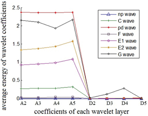
Both amplitude and frequency of the EPG signal are characterized as non-stationary signals altering with time. Wavelet transformation could split the signals into varied frequency constituents or distinct-scale constituents (Khokhar et al. 2017). Thus, the coefficients of the wavelet could designate the energy distribution of the signal in the time-frequency domain. Moreover, the energy of wavelet coefficients is derived from the time-frequency attributes of the waveforms of EPG (Xing et al. 2022). The feature extraction method of the wavelet energy for the EPG waveforms is conducted based on the steps: 1. $C_{j,k}$, the coefficients of wavelet decomposition in each layer, are attained by decomposing the $j$-layer wavelet of signals of EPG. 2. The mean energy distribution in each decomposition layer is computed. Namely, Equation 33(32) $Untargeted:\mathrm{m}\mathrm{i}{\mathrm{n}}_{\mathrm{x}{ }^{\mathrm{\prime }}}\mathrm{d}\left(\mathrm{x}{ }^{\mathrm{\prime }},\mathrm{x}\right)\mathrm{s}\mathrm{u}\mathrm{b}\mathrm{j}\mathrm{e}\mathrm{c}\mathrm{t}\mathrm{t}\mathrm{o}\mathrm{C}\left(\mathrm{x}{ }^{\mathrm{\prime }}\right)\ne \mathrm{C}\left(\mathrm{x}\right)$(32) shows the computational procedure, which consists of squaring the decomposition coefficients of each layer, then all are summed up.

(24) $E_j=\frac{{\sum }_{k=0}^{N_j}{(C_{j,k})}^2}{N_j}$(24)

Where the number of the decomposition layers is denoted by $j$ and $N_j$ represents the distance of the coefficients of the wavelets in the $j$ -th layer. (3) The mean energy in each layer is picked. Then, the attribute vector was formed.

Because 100 Hz is picked as the frequency of the sampling of the EPG signal and the frequencies of varied waveforms of EPG are generally condensed between 2 and 20 Hz, the wavelet decomposition of the EPG signal is denoted by the 6-layer “sym4” conducted in the experiment. Figure 3 depicts that the mean energy of the high and low-frequency coefficients between 2 and 5 layers is derived. The 100 samples having the average wavelet energy concerning seven kinds of EPG are presented between A2 through A5 graphs that characterize the low-frequency coefficients of the wavelet decomposition between the second through fifth ones. Thus, the high-frequency coefficients of the second- and fifth-layer wavelet decomposition are represented between D2 through D5. Thus, the LFE part has various EPG waveforms altering to a great extent. However, the high-frequency energy section has much less varying EPG waveforms. Accordingly, other attributes are fused with the low frequency mean energy part to construct the attribute vector.

Figure 3. Average energy contrast of wavelet coefficients in layers 2~5.

The Features of a Fractal Dimension

The word fractal is termed to be used to represent the class of structures having large complexness and no defined distance for the attribute but self-similarity. A significant index called fractal dimension is employed to measure fractal, which is extensively employed to quantitatively describe the behavior of non-linearity (Xiong, Zhang, and Yang 2012).

The signal of EPG is described as a type of time series data. So, the FD could efficiently represent its alterations, complex structure of the distribution, and abnormalities. Then, both the BD and the HE are picked as the attributes of the fractal dimension to reduce the complexity of the computations.

Box Dimension (BD)

Suppose that X denotes any non-empty bounded subset in Rⁿ, and N_δ(X) denotes the smallest number of covering X classes with the maximum radius δ. Equation 33(32) $Untargeted:\mathrm{m}\mathrm{i}{\mathrm{n}}_{\mathrm{x}{ }^{\mathrm{\prime }}}\mathrm{d}\left(\mathrm{x}{ }^{\mathrm{\prime }},\mathrm{x}\right)\mathrm{s}\mathrm{u}\mathrm{b}\mathrm{j}\mathrm{e}\mathrm{c}\mathrm{t}\mathrm{t}\mathrm{o}\mathrm{C}\left(\mathrm{x}{ }^{\mathrm{\prime }}\right)\ne \mathrm{C}\left(\mathrm{x}\right)$(32) represents the BD of X by

(25) $F_B=\underset{\delta \to \mathrm{\infty }}{lim}\frac{log{N}_{\delta }(X)}{log(1/\delta )}$(25)

Resolving the limit presented in Equation 33(32) $Untargeted:\mathrm{m}\mathrm{i}{\mathrm{n}}_{\mathrm{x}{ }^{\mathrm{\prime }}}\mathrm{d}\left(\mathrm{x}{ }^{\mathrm{\prime }},\mathrm{x}\right)\mathrm{s}\mathrm{u}\mathrm{b}\mathrm{j}\mathrm{e}\mathrm{c}\mathrm{t}\mathrm{t}\mathrm{o}\mathrm{C}\left(\mathrm{x}{ }^{\mathrm{\prime }}\right)\ne \mathrm{C}\left(\mathrm{x}\right)$(32) is practically difficult. Therefore, an approximation methodology is adopted to compute. A series of square grids are utilized to cover the scale-free area of the discrete signal represented by X(n),

The utilization of the x-grid leads a scale to be incrementally expanded to a grid denoted by kδ to attain grid numbers N_kδ covered by each scale. Afterward, the LS approach is employed to attain the estimated function of logkδ−logN_kδ. So, its inclination shows the FBD F_B of the discrete signal denoted by X(n).

The BD of the EPG signal ranging between 1 and 2 is found. So, the more complicated the waveform is, the greater the BD would be

The Hurst Exponent (HE)

H, called the HE, is an estimation of the self-similarity measurement with no dimension (Lahmiri 2018), which is generally utilized to designate the correlated time series in a long run. When H is assigned to 0.5, it is characterized as inapplicable or pertinent to a very short run. When H is larger than 0.5, it represents a substantial positive correlation and is sturdy. When H is less than 0.5, it represents a long-run correlation. However, the whole trend is in the reverse direction, namely, anti-persistence exists.

Once the HE is estimated, the generally applied approach is called the R/S procedure, which is also called rescaled range analysis. X(n) denotes time series whose domain is split into subintervals with equal length N, and the HE series is attained by running calculations repeatedly for each subinterval. Thus, Equation 33(32) $Untargeted:\mathrm{m}\mathrm{i}{\mathrm{n}}_{\mathrm{x}{ }^{\mathrm{\prime }}}\mathrm{d}\left(\mathrm{x}{ }^{\mathrm{\prime }},\mathrm{x}\right)\mathrm{s}\mathrm{u}\mathrm{b}\mathrm{j}\mathrm{e}\mathrm{c}\mathrm{t}\mathrm{t}\mathrm{o}\mathrm{C}\left(\mathrm{x}{ }^{\mathrm{\prime }}\right)\ne \mathrm{C}\left(\mathrm{x}\right)$(32) is used to compute the Hurst exponent.

(26) $log\frac{R\left(N\right)}{S\left(N\right)}=HlogN+C$(26)

where C and R/S denote a constant and a rescaled interval. The inclination coefficient of the function called regression is equal to the predicted score of the HE when$log\frac{R\left(N\right)}{S\left(N\right)}$ and logN are regressed by utilizing the LS approach (Ma et al. 2018).

The experimentation computes both BD and HE of the waveforms of EPG based on one hundred samples as their attributes with nonlinearity property. Table 2 presents the mean BD and the HE that utilizes 100 samples for presentational purposes.

Table 2. The attributes of the FD of the waveforms in EPG.

Waveforms	Box dimensions	Hurst exponents
np	1.566	0.063
pd	1.343	0.672
E1	1.44	0.261
E2	1.506	0.141
G	1.64	0.723
C	1.514	0.247
F	1.689	0.494

Table 2 presents the scores of both E2 and the C waves that are suchlike in the BD attribute. The scores of both E1 and the C waves are also not much distinct in the HE attributes. Thus, the characteristics of the fractal dimension for other waveforms are distinct and can be employed as grouping attributes.

The Features of the Hilbert – Huang Transformation (HHT)

The HHT comprises both EMD and HT and primarily conducts the EMD employing signals to attain the addition of many IMF. Afterward, both instant frequency and amplitude of the signal are attained by conducting the HT on each IMF constituent. Finally, the Hilbert spectrum of the signal is attained (Nalband et al. 2018; Yan and Lu 2014). To decrease the complexness of the computation, the SC is implemented as an HHT attribute in the attribute derivation of EPG.

Equation 33(32) $Untargeted:\mathrm{m}\mathrm{i}{\mathrm{n}}_{\mathrm{x}{ }^{\mathrm{\prime }}}\mathrm{d}\left(\mathrm{x}{ }^{\mathrm{\prime }},\mathrm{x}\right)\mathrm{s}\mathrm{u}\mathrm{b}\mathrm{j}\mathrm{e}\mathrm{c}\mathrm{t}\mathrm{t}\mathrm{o}\mathrm{C}\left(\mathrm{x}{ }^{\mathrm{\prime }}\right)\ne \mathrm{C}\left(\mathrm{x}\right)$(32) defines the SC which is called the epicenter of the frequency constituent distribution of the signal.

(27) $S{C}_i=\frac{{\sum }_{j=1}^M{f}_i\left(j\right)E_i\left(j\right)}{{\sum }_{j=1}^M{E}_i\left(j\right)}$(27)

Where the signal length is denoted by M, and f_i(j) and E_i(j) denote the immediate frequency and energy scores at the jth sampling datum of the ith IMF constituent.

Since the immanent attributes of the signal are generally presented in the first few IMF constituents, and the latter ones mainly include less information, the spectral centroids of the first two IMF constituents are derived as attributes of the HHT. So, Table 3 summarizes the average spectral centroid of the first four layers of the EPG waveforms having 100 data.

Table 3. The HHT attributes of the EPG waveforms.

Characteristic values	The spectral centroid of the first layer	The spectral centroid of the second layer	The spectral centroid of the third layer	The spectral centroid of the fourth layer
np	0.296	0.135	0.059	0.025
pd	0.156	0.074	0.038	0.021
E1	0.099	0.065	0.046	0.029
E2	0.166	0.072	0.043	0.022
G	0.140	0.052	0.035	0.019
C	0.162	0.076	0.044	0.021
F	0.136	0.081	0.049	0.023

Table 3 depicts the various outcomes between different waveforms such as E2, C, G, and F waves that were 0.04 when the values related to the first layer spectral centroid characteristics are under consideration. There exists a difference between the pd and E2 waves, which is 0.02 in spectral centroid representation scores of the second layer. When spectral characteristics of the third layer are under consideration, there exists a difference between the E2 and C waves, which is 0.001; there exists a difference between the pd and C waves in the fourth one, which is zero. While the disparity between waveforms tends to decrease, the number of layers increases. The third and fourth layers having the HHT attributes are not found useful to classify the EPG waveforms.

The Attribute Vector of the EPG Waveforms

The combinations of five distinct attribute vectors are employed to make the comparison. The first class of attributes, S1, consists of LFWE in both the second and fifth layers, the BD, and the HE, and contains six attributes in total. The second class of attribute vectors, S2, consists of the same WE in both second and the fifth layers as S1 and SC in the first two layers of the HHT and contains six attributes in total. The third class of attribute vectors, S3, consists of the same wavelet energy in the second and the fifth layers, the BD, the HE, and the spectral centroid in the first two layers of the HHT and includes eight attributes in total. The fourth class of attributes vectors, S4, consists of the same wavelet energy in the second and the third layers, the BD, the HE, and the SC in the first two layers of the HHT and includes six attributes in total. Finally, the fifth class of attribute vectors, S5, consists of the same wavelet energy in the fourth and the fifth layers, the BD, the HE, and the SC in the first two layers of the HHT and contains six attributes in total.

Wu et al. employed both the same training and test samples and classifiers to make comparisons with the outcomes of the prior studies. Table 4 summarizes the outcomes of combining various attributes.

Table 4. Comparing detection rates of decision trees with the distinct attribute vector.

Recognition rates（%）	Attribute vector
	S1	S2	S3	S4	S5
Group 1	85.00	81.43	90.00	91.43	90.00
Group 2	87.14	80.71	90.00	90.00	89.29
Group 3	97.14	93.57	93.57	93.57	93.57
Group 4	94.29	90.71	91.43	91.43	92.86
Mean（%）	90.90	86.61	91.25	91.61	91.43

Table 4 presents that the mean recognition ratio attained by employing the combination of the S4 attribute vector is found to be the maximum at 91.61%. The mean recognition ratio attained by the combination of the S5 attribute vector is the same as that of the previously conducted experiments with 91.43% (Wu et al. 2018). Accordingly, the combination of S4 is employed as the attribute vector of the WKELM classifier in the manuscript.

Figure 4 depicts the attribute distribution of 7 different types of EPG waveforms with 100 samples. The WE in both second and the third layers, BD, and the second layer SC of the G wave was found to be relatively condensed, sturdy, less bisecting with other attributes, and simple to separate. The spectral centroid is defined as a metric to characterize a spectrum in the processing of digital signals, characterizing the location of the mass center of the spectrum, having a sensible perceptual connection with the perception of the brightness of a sound, and is also known as the center of spectral mass. The BD and the second layer SC of the F wave were found to be consistent.

Figure 4. Features distribution of EPG waveforms.

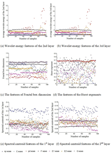
Hence, the Hurst exponent attributes of the pd are condensed. The HE exponent is employed as a magnitude for the long-run memory of time series. It concerns time series autocorrelations and how they reduce as the latency between data pairs grows. The Hurst exponent was first used in hydrology to determine the size of the best dam for the varying rain and drought requirements of the Nile River, which were researched in the long run. Besides, the second layer SC attributes of the np do not intersect with others and were simple to segregate, which could be employed for the WKELM classifier as input vectors and its result is 7-kind waveforms of EPG. It must be noted that a wavelet is an oscillating structure with a wave-like amplitude whose starting point is zero, then increases or decreases, and afterward goes back to zero once or more than once.

Wavelets as “brief oscillations” have a taxonomy depending on the number and direction of their pulses and also have unique features that make them valuable for signal processing.

The Classification of the EPG Waveforms Utilizing the WKELM

Seven types of waveforms, namely, np, pd, C, E1, E2, F, and G waves available in the signal of EPG are clustered in the experiment. The S4 is employed as the attribute vector for the WKELM classifier to input, and four groups of experiments conducted are the same as the samples in the literature (Wu et al. 2018). Once the WKELM as a classifier is employed, the first affinity weights and the thresholds of the hidden layer are assigned randomly. To assure the stable outcome of each grouping, the weights and thresholds are kept constant, and the same random scores are implemented in each process. The number of hidden layers has a considerable impact on the results of the grouping. Figure 5 depicts the detection ratio of the classification concerning the four groups of the experimental data when the neuron numbers altered between 20 and 400. Neuron numbers are not the more the better situation. While neuron number goes up, the detection ratio lowers.

Figure 5. The impact of the neuron numbers in the hidden layer on the achievement of the ELM Classification.

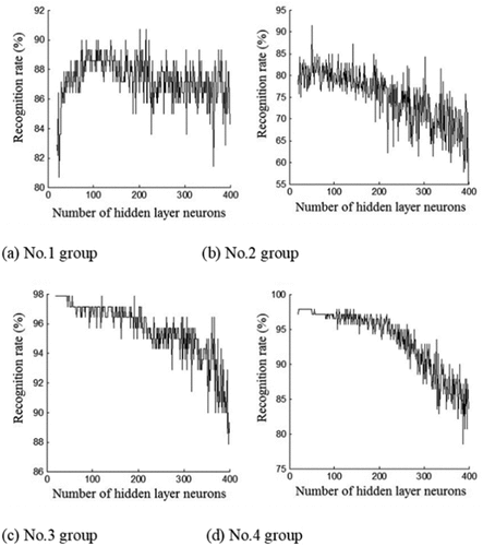
How many neurons are needed to attain the best classification outcomes regarding the hidden layer of the WKELM is still an open issue that needs theoretical treatment. To attain the best recognition ratio, the incremental method is implemented to choose the number of neurons in the hidden layer adaptively when the experiment is run. Hence, the optimized network edifice is found by raising the number of neurons in the hidden layers one at a time (Huang and Chen 2008). After each iteration accepts new neurons, the updated weights and anticipated errors of the available neurons in hidden layers are recalculated until the residuals converge to the preset scores.

The term “preset scores” refer to a predetermined threshold or criteria used to determine when the algorithm has converged to an acceptable solution. For example, the algorithm is set to continue adding new neurons to the hidden layer until the residual errors fall below a certain threshold or until a certain number of neurons have been added. The precise method for setting these preset scores depends on the specific ELM, dataset, and the application’s goals.

In the context of the proposed ELM, the term “preset scores” refer to the threshold value for the training error and the norm of the output weights. We set the value of this threshold as a stopping criterion for the ELM algorithm.

The training error threshold is typically defined as the maximum allowable difference between the desired output and the actual output of the ELM. This value is usually set based on the desired accuracy of the model and the available computational resources. Once the training error falls below this threshold, the algorithm is stopped and the resulting model is considered trained.

The norm of the output weights threshold is another stopping criterion that can be used to terminate the ELM algorithm. In this case, the algorithm is stopped when the norm of the output weights exceeds a certain threshold value. This criterion is typically used to prevent overfitting of the ELM model, where the model becomes too complex and begins to fit the training data too closely.

In both cases, the threshold values are set by the user and are considered to be “preset scores” that determine when the algorithm has converged to an acceptable solution. The precise values of these thresholds may depend on the specific application and the goals of the ELM model.

Hence, the smallest number of neurons in the hidden layer and the parameters of the neurons in each hidden layer are attained.

Adversarial Examples

By conducting several transformations, intelligent models cause problem-solving, for example, pattern recognition. Most of these transformations are very delicate to small perturbations in the input, so exploiting this delicateness could cause them to modify their behavior under these circumstances. In addition, each learning algorithm has some specific bias, such as in the hyperparameters it uses, the methodology of separating and ranking the classes, or the ways of representing the information. Accordingly, the training data used, because it is finite, does not precisely designate reality, as its selection process and assumption on the data set having the same distribution as the set of unknown cases lead to another level of bias. Hence, intelligent algorithms could be vulnerable to specialized offenses.

Therefore, designing suitable inputs in a certain way leads the learning algorithm to wrong transformations, producing bad results. These attacks are called adversarial attacks and are a significant issue in the dependability of artificial intelligence approaches. The learning methods were proposed by assuming that training and test datasets are drawn from the same distribution, which is unknown in advance. For instance, a trained neural network characterizes a long-range decision boundary that corresponds to a standard class. This bound is not perfect, and a properly devised and utilized attack, which corresponds to an altered input that generally comes from slightly different data, could cause the method to classify wrongly (wrong class).

Completely connected neural networks consist of layers of artificial neurons. Neurons receive input from prior layers, crunch it by using an activation mapping and transfer it to the next one at each layer. While sample x denotes the input of the first layer, and the result $F\hspace{0.17em}\left(x\right)$ is the outcome of the last layer. A fully connected m-level neural network could be constructed based on the equation:

(28) $z^{\left(0\right)}=x;z^{\left(l+1\right)}=\sigma \left(W^l{z}^l+b^l\right)$(28)

The classifier is defined by the attack to describe the objective of the function as follows:

(29) $f:[0,1{]}^d\to {\mathbb{R}}^K$(29)

Scenario 1

The aim of this offense is defined by

(30) $\mathrm{a}\mathrm{r}\mathrm{g}\mathrm{m}\mathrm{a}{\mathrm{x}}_{k=1,\dots ,K}{f}_k\left(\hat{x}\right)\ne y,\parallel \hat{x}-x{\parallel }_p\le \text{isin}\mathrm{a}\mathrm{n}\mathrm{d}\hat{x}\in [0,1{]}^d$(30)

Scenario 2

The objective of this offense is defined by

(31) $\mathrm{T}\mathrm{a}\mathrm{r}\mathrm{g}\mathrm{e}\mathrm{t}\mathrm{e}\mathrm{d}:\mathrm{m}\mathrm{i}{\mathrm{n}}_{x{ }^{\mathrm{\prime }}}d\left(x{ }^{\mathrm{\prime }},x\right)\mathrm{s}\mathrm{u}\mathrm{b}\mathrm{j}\mathrm{e}\mathrm{c}\mathrm{t}\mathrm{t}\mathrm{o}C\left(x{ }^{\mathrm{\prime }}\right)=c^{\ast }$(31)

(32) $Untargeted:\mathrm{m}\mathrm{i}{\mathrm{n}}_{\mathrm{x}{ }^{\mathrm{\prime }}}\mathrm{d}\left(\mathrm{x}{ }^{\mathrm{\prime }},\mathrm{x}\right)\mathrm{s}\mathrm{u}\mathrm{b}\mathrm{j}\mathrm{e}\mathrm{c}\mathrm{t}\mathrm{t}\mathrm{o}\mathrm{C}\left(\mathrm{x}{ }^{\mathrm{\prime }}\right)\ne \mathrm{C}\left(\mathrm{x}\right)$(32)

The Outcomes of the Experiment and the Analysis

The motivation behind this paper is to improve the security of machine learning algorithms, especially in scenarios where authorized implementers and eavesdroppers are close to each other, which can lead to errors in beamforming and beam leakages. The paper aims to address this issue by proposing a framework called the WEPF, which incorporates non-orthogonality into the physical layer signal waveform.

The paper focuses on the categorization of the EPG for insects, which is used in the study of insect feeding behavior and the transmission of viruses between insects. The proposed framework was tested using a six-dimensional attribute vector, which included features such as low-frequency wavelet energy, fractal box dimension, Hurst exponent, and spectral centroid. The results showed that the WEPF was effective in preventing eavesdropping or tampering with the waveforms used in advanced machine learning methods in two adversarial scenarios.

Overall, the motivation of this paper is to provide a solution to the difficulty in performing secure beamforming in waveform applications and to enhance the security of machine learning algorithms against adversarial attacks.

To exemplify the efficacy of the WKELM when the EPG waveforms are classified, distinct classifiers are employed to compare the outcomes. A DC, probabilistic NNs, the ELM, radial basis function ELM, polynomial kernel ELM, and the classifier called WKELM employ the same samples as input. Table 5 finally summarizes the recognition outcomes.

Table 5. Comparing the recognition outcomes of the diverse classifiers.

	Distinct Classifiers	No.1 group	No.2 group	No.3 group	No.4 group	Mean（%）
Recognition rate（%）	Decision Tree	91.43	90.00	93.57	91.43	91.61
	PNN	85.71	82.86	97.86	96.43	90.72
	ELM	90.71	87.86	97.86	97.86	93.57
	RBFELM	90.00	88.57	97.86	97.86	93.57
	PKELM	90.71	87.14	97.86	97.86	93.39
	WKELM	90.71	91.43	97.86	97.86	94.47

The mean classification outcomes derived from utilizing the 4 group data sets are depicted in Table 5. While the recognition ratio of PNN is found to be the smallest at 90.72%, and the recognition ratio of the WKELM is found to be the maximum at 94.47%. The multi-scale approximation features of the wavelet function are inherited from the wavelet kernel function, so a better impact on the outcomes of the classification is achieved.

While the recognition ratios of groups 1 and 2 are found to be lower, the recognition ratios of groups 3 are found to be higher when no matter which classifier is employed based on single group experiment data set. Why large differences in the classification outcomes are reached can be summarized as follows:

1. Outside interference and the insects corrupt EPG signals, which are biological signals. Even though they come from the exact waveform, both amplitude and frequency would alter. The C wave particularly presents this situation. There exists a difference between the waveform directions between the first and the next hours, which results in the dissipation of the derived attribute scores and misjudgments in classification outcomes.

2. The experiment utilizes a method that classifies objects employing a framework, which is called supervised learning. If the model is not trained with large samples, the recognition rate will be lower when both training and test samples differ largely.

It must be said that this thorough research and the context in which the experiments were carried out is the first of its kind, and there is no equivalent to conducting comparisons.

Conclusion

This investigation took place during the first phase of this project. During this effort, our research and study concentrated on studying a specialized assault scenario and determining how resistant it would be too universal counterexample detection approaches based on the suggested WEPF. During the second stage of this research project, we used the second scenario to investigate the power and efficiency of combined assault methods. The fact that the methodology produced very high outcomes in both examples, as was shown through the use of experiments, demonstrates its usefulness and efficiency.

In the past, recognizing waveforms in investigations into insects and plants that involved using EPG equipment was always done by hand. This practice continues today. Due to the complex waveforms of the electroencephalogram, ECG, and other techniques of processing bioelectrical signals, the application of machine learning to detect the waveforms of the electroencephalogram runs more slowly than those other methods.

The attribute derivation and grouping methodologies of the EPG waveforms of aphids are investigated in the study. It has been determined how to construct the attribute vector that combines WE, FD, and HHT. After that, a classifier that is based on WKELM is utilized. Following that, a mean recognition ratio of 94.47% is achieved, which is 3.04% higher than the previous research carried out, and its mean recognition ratio is 91.43%. Then, the mean recognition ratio of 91.43% is achieved (Wu et al. 2018). The results of the studies indicate that the proposed WKELM classifier is a more workable method for classifying the EPG waveforms.

Because of the convergence of data, algorithms, and computation, the suggested framework enjoys high trust. This is because it demonstrated outstanding performance on a variety of experiments that were carried out, each including specifically outlined scenarios.

The following is a condensed summary of the constraints and the potential next steps for this line of research: The only topic covered in this publication is the automatic classification of EPG waveforms; nevertheless, several study fields still need to be developed further.

1. There are only seven different kinds of waveforms known.

2. While thinking about the transmission of a virus, it is necessary to consider the recognition of the waveform represented by E1 + E2. This allows for the derivation of the characteristics essential to the time-frequency domain and nonlinearity. It should be noted that other characteristics associated with time and frequency domains could probably improve the ratio of the recognition rates, which necessitates more verifications.

3. More experimental research is required to assess whether or if the random forest method, an example of an integrated learning classifier, could yield a higher recognition ratio.

Some possible future directions for this work and related research in this field could be:

1. Extension of the proposed framework to other machine learning applications and scenarios, such as image or speech recognition, natural language processing, and autonomous systems.

2. Investigating the performance of the proposed framework under different types of adversarial attacks, including those specifically designed to bypass the non-orthogonality idea in the physical layer signal waveform.

3. Exploring the potential impact of the proposed framework on the accuracy and efficiency of machine learning algorithms.

4. Developing methods to improve the interpretability and transparency of machine learning algorithms while maintaining their security.

5. Investigating the trade-offs between security, accuracy, interpretability, and efficiency in machine learning algorithms, and identifying optimal solutions for different applications and scenarios.

6. Integrating the proposed framework with other security mechanisms, such as encryption and authentication, to provide a more comprehensive security solution for machine learning algorithms.

Overall, the proposed framework and related research in this field have the potential to make significant contributions to the development of secure and trustworthy machine learning algorithms, which are essential for many critical applications in today’s society.

In conclusion, in this paper, we proposed a WEPF to improve the security of machine learning algorithms in scenarios where eavesdropping and manipulation of waveform signals are possible. The framework incorporates a non-orthogonality idea into the physical layer signal waveform, which was able to successfully secure all waveform signals in two adversarial scenarios. The proposed framework was tested using an attribute vector with 6 dimensions in the application scenario of classifying EPG signals for insects. However, future research is needed to extend the framework to other machine learning applications and scenarios and investigate its performance under different types of adversarial attacks. The development of secure and trustworthy machine learning algorithms is essential for many critical applications in today’s society, and the proposed framework and related research in this field have the potential to make significant contributions to this goal.

Ethical approval

The research did not contain any subjects of humans or animals; thus, there exists no approval required regarding ethical standards.

Preprint

A preprint has previously been published.

Acknowledgements

The contributors gratefully acknowledge Francisco Adasme-Carreño and his research crew for their EPG database and software.

Disclosure statement

No potential conflict of interest was reported by the authors.

Data availability statement

The data used in the research are available from the author upon request.

Additional information

Funding

The research was patronized by the Science and Technology Department of Henan Province (grant number 182102110334), the Key Scientific Research Project of Colleges and Universities in Henan Province (grant number 18A510012), and the Science and Technology Innovation Fund of Henan Agricultural University (grant number KJCX2017A19 and KJCX2018A20).

References

- Adasme-Carreño, F., C. Muñoz-Gutiérrez, J. Salinas-Cornejo, and C. C. Ramírez. 2015. A2EPG: A new software for the analysis of electrical penetration graphs to study plant probing behavior of hemipteran insects. Computers and Electronics in Agriculture 113:128–1470. doi:10.1016/j.compag.2015.02.005.
- Alba-Tercedor, J., W. B. Hunter, and I. Alba-Alejandre. 2021. Using micro-computed tomography to reveal the anatomy of adult Diaphorina citri Kuwayama (Insecta: Hemiptera, Liviidae) and how it pierces and feeds within a citrus leaf. Scientific Reports. 11(1):1–30. doi:10.1038/s41598-020-80404-z.
- Backus, E. A., H. T. Shih, and P. Weintraub. 2020. Review of the EPG waveforms of sharpshooters and spittlebugs including their biological meanings in relation to transmission of Xylella fastidiosa (Xanthomonadales: Xanthomonadaceae). Journal of Insect Science 20 (4):6. doi:10.1093/jisesa/ieaa055.
- Cornara, D., E. Garzo, M. Morente, A. Moreno, J. Alba-Tercedor, and A. Fereres. 2018. EPG combined with micro-CT and video recording reveals new insights into the feeding behavior of Philaenus spumarius. PLos One 13 (7):e0199154. doi:10.1371/journal.pone.0199154.
- Diker, A., D. Avci, E. Avci, and M. Gedikpinar. 2019. A new technique for ECG signal classification genetic algorithm wavelet kernel extreme learning machine. International Journal for Light and Electron Optics 180:46–55. doi:10.1016/j.ijleo.2018.11.065.
- Ebert, T. A., E. A. Backus, M. Cid, A. Fereres, and M. E. Rogers. 2015. A new SAS program for behavioral analysis of electrical penetration graph data. Computers and Electronics in Agriculture 116:80–87. doi:10.1016/j.compag.2015.06.011.
- Huang, G. B. 2015. What are extreme learning machines? filling the gap between frank rosenblatt’s dream and John von Neumann’s puzzle. Cognitive Computation 7 (3):263–78. doi:10.1007/s12559-015-9333-0.
- Huang, G. B., and L. Chen. 2008. Enhanced random search based incremental extreme learning machine. Neurocomputing 71 (16–18):3460–68. doi:10.1016/j.neucom.2007.10.008.
- Jallingii, W. F. 1978. Electronic recording of penetration behavior by aphids. Entomologia Experimentalis et Applicata 24:721–30.
- Jing, P., S. F. Bai, and F. Liu. 2013. Research progress on EPG waveform types analysis on the feeding behavior of common piercing-sucking insects. China Plant Protection 4:18–23.
- Khokhar, S., A. A. M. Zin, A. P. Memon, and A. S. Mokhtar. 2017. A new optimal feature selection algorithm for classification of power quality disturbances using discrete wavelet transform and probabilistic neural network. Measurement 95:246–59. doi:10.1016/j.measurement.2016.10.013.
- Lahmiri, S. 2018. Generalized Hurst exponent estimates differentiate EEG signals of healthy and epileptic patients. Physica A Statistical Mechanics & Its Applications 490:378–85. doi:10.1016/j.physa.2017.08.084.
- Ma, Y., W. B. Shi, C. K. Peng, and A. C. Yang. 2018. Nonlinear dynamical analysis of sleep electroencephalography using fractal and entropy approaches. Sleep Medicine Reviews 37:85–93. doi:10.1016/j.smrv.2017.01.003.
- Nalband, S., C. A. Valliappan, A. Amalin Prince, and A. Agrawal. 2018. Time-frequency-based feature extraction for the analysis of vibroarthographic signals. Computers & Electrical Engineering 69:720–31. doi:10.1016/j.compeleceng.2018.02.046.
- Prado, E., and W. F. Tjallingii, 1994. Aphid activities during sieve element punctures. Entomol. Exp. Appl. 72, 157–65T.
- Tjallingii, W. F. 1985. Electrical nature of recorded signals during stylet penetration by aphids. Entomologia Experimentalis Et Applicata 38 (2):177–86. doi:10.1111/j.1570-7458.1985.tb03516.x.
- Tjallingii, W. F. 2014. EPG Systems. http://www.epgsystems.eu/products.php.
- Tjallingii, W. F., and T. H. Esch. 1993. F1993. Fine structure of aphid stylet routes in plant tissues in correlation with EPG signals. Physiological Entomology 18 (3):317–28. doi:10.1111/j.1365-3032.1993.tb00604.x.
- Wu, L., S. Jia, Y. Xing, S. Lu, J. Pan, and F. Yan. 2018. Machine identification of electrical penetration graphic waveforms of aphid based on fractal dimension and Hibert-Huang transform. Transactions of the Chinese Society of Agricultural Engineering 24:175–83.
- Xing, Y., B. Li, L. Wu, and F. Yan. 2022. Aphid EPG waveforms classification based on wavelet kernel extreme learning machine. doi:10.21203/rs.3.rs-1484523/v1.
- Xiong, G., S. N. Zhang, and X. N. Yang. 2012. The fractal energy measurement and the singularity energy spectrum analysis. Physical A 391 (24):6347–61. doi:10.1016/j.physa.2012.07.056.
- Xu, T. (2020). Waveform-defined security: A framework for secure communications. 2020 12th International Symposium on Communication Systems, Networks and Digital Signal Processing (CSNDSP).
- Xu, T. (2021). Waveform-defined privacy: A signal solution to protect wireless sensing. 2021 IEEE 94th Vehicular Technology Conference (VTC2021-Fall), pp. 1–5
- Yan, J. H., and L. Lu. 2014. Improved Hilbert–Huang transform-based weak signal detection methodology and its application on incipient fault diagnosis and ECG signal analysis. Signal Processing 98:74–87. doi:10.1016/j.sigpro.2013.11.012.