Air Quality Index Prediction Using DNN-Markov Modeling

ABSTRACT

Air quality measurements contribute to diverse socio-economic sectors, including the environment and healthcare. Many methods are commonly applied to present air-quality levels, reflecting differing national standards. This study presents an air quality index prediction model, to measure air pollution levels for healthcare applications in congested areas. DNN-Markov modeling techniques are used to predict air quality, based on environmental conditions at peak hours. The developed model presents different approaches for highly accurate prediction of the air quality index for the next hour at a given location, under specific environmental conditions. This system could be used to support planning decisions related to the consequences of air quality. The study was conducted in selected locations in Jordan and England as a comparative model prediction accuracy study using different big-data sets of multivariate time series in traffic-heavy locations. The air quality index was represented using Neuro Fuzzy Logic as a method to contribute in air quality index predictions within blurry (boundary) values. The selected DNN-Markov hybrid model could predict air quality with accuracy of around (RMSE 7.86) for the location in England, and around (RMSE 15.27) for the one in Jordan.

Introduction

Air quality prediction involves various factors, intricately connected to atmospheric conditions and exhibiting time dependencies. The concentrations of air pollutants are influenced by meteorological events and state fluctuations, and optimal forecasting in specific domains is hampered by the limited availability of valid air-quality datasets (Tripathi and Pathak 2021). Nevertheless, there is increasing urgency to address high pollutant levels and their consequences, which has elicited in-depth studies on air quality parameters, temporal dimensions, and spatial interactions (Alnawaiseh and Hashim 2014; Cheng et al. 2007; Masih 2019). Emissions, being a complex mixture of gases and meteorological conditions, present challenges for forecasting models due to non-linearity and a lack of meteorological parameters in certain regions (Masih 2019). Air quality is affected by multiple complex factors, such as traffic flow, meteorology, and land use, and the data are not sufficient and accurate to model each factor which present challenges in prediction. Moreover, there are some very sharp changes which can be caused by unusual weather conditions (inflection points) and significant variations in air pollution because air itself changes over location and time. Given the plethora of instrumental variables, current tools for the generic prediction of overall air quality are not useful for decision-making (Zheng et al. 2015).

Machine Learning Approaches and Challenges

Tealab (2018) used systematic review method to address air quality prediction challenges, exploring the use of Neural Networks (NN), Support Vector Machines (SVM), and the Ensemble Learning algorithm, known for their ability to capture non-linearity in modeling. Analyzing research on air quality prediction indicates that NNs are among the most reliable and cost-effective machine-learning tools, but issues such as overfitting and generalization have been identified with their use (Siami-Namini, Tavakoli, and Namin 2019). While some of these issues were resolved using other methods such as SVM, linear regression, and many other linear and non-linear methods (Méndez, Merayo, and Núñez 2023), the existing literature still debates suitable methods for air quality prediction, and discusses more possibilities of combined solutions that could overcome shortages in stand-alone models (Devasekhar and Natarajan 2023; Masih 2019).

The extensive literature on time-series Artificial Neural Network (ANN) research underscores the efficiency of NNs, but its use still depends on modelers’ experience, and lacks systematic procedures, particularly for non-linear forecasting in time series (Baatarchuluun, Sung, and Lee 2020; Niska et al. 2004; Shrestha and Mahmood 2019). Tealab’s (2018) systematic review of time-series forecasting revealed that many studies utilized hybrid (linear and non-linear) models. Despite the importance of traditional predictive modeling methods like ARIMA, SARIMA, ARIMAX, and other statistical linear modeling, the need for deep learning arises to better capture non-linearity in data between parameters, ensuring reliable performance and accuracy in time-series data (Siami-Namini, Tavakoli, and Namin 2019).

Deep Neural Networks (DNN) Evolution

In the evolution of DNN, the Universal Approximation Theorem initially posed challenges, but the emergence of the backpropagation learning algorithm marked a significant leap for DNN. This advancement automated feature extractors, providing added value compared to traditional machine-learning techniques. Despite such progress, deep learning algorithms had their shortcomings, prompting the development of various architectures and training techniques as revolutionary solutions (Kaur et al. 2023).

An increase in the number of layers within DNNs enhanced their capacity for network learning. However, this did not necessarily lead to an improvement in accuracy (Barrera-Animas et al. 2022). Shifting focus to air pollution time-series prediction, traditional statistical linear methods have been employed in the past, but recent research has explored the use of various combined machine-learning methods for air-quality forecasting over the past decade (Shrestha and Mahmood 2019).

Discrete Time Series and Advanced Models

The complex nature of air-quality prediction, coupled with variations in data sources and parameters, underscores the urgent need for accurate measurement methods. This highlights the necessity for further research to enhance air-quality prediction (Ameer et al. 2019). Time series offer multiple approaches for forming models, with discrete-valued time series finding application in various contexts. Discrete models require careful consideration of the data’s discrete nature when building distributions, emphasizing that a normal distribution may not always be the optimal choice (Ameer et al. 2019).

The Markov-switching dynamic regression model marked a breakthrough in work on state-space representation. Introduced in 1988–89, it represented the dynamic behavior of time-series variables, with switching represented by a DTMC object (Kim 1994). The Markov-switching vector autoregressive (MS-VAR) model, considered a complex application, was proposed by Iain and MacDonald (2016) as a solution for non-linear time-series models. Finite-state Markov chains form a discrete-time stochastic process transitioning between states. Predictions in this process depend on the immediate past, emphasizing the sequence of previous states. Markov chains neglect past information, but use the outcome of the most recent experiment to predict the future, describing a process of transitioning between states with transition probabilities (Kemeny and Snell 1983).

This paper discusses the revolution of air quality prediction and the complexities related to the domain, presenting the shift from statistical linear methods to more advanced machine learning methods, and addressing the limitations of some of the most used algorithms in the domain, such as ANNs, DNNs, and some others. This paper addresses some of the limitations and drawbacks of some algorithms which are dominant in the field of air quality forecasting, and presents hybrid modeling as a solution of integrated way to overcome some shortages of stand-alone algorithms. Moreover, it concludes that integrating traditional statistical methods with advanced machine learning unlocks the potential for improving air quality prediction accuracy. This paper presents the contribution of integrating DNNs model with Markov-switching dynamic regression model as hybrid modeling for air quality prediction with the aim of achieving suitable accuracy within the introduced framework.

Real-World Relevance and Practical Implications of Air Quality Prediction Research

A bibliometric review of 100 studies over 20 years have been performed in an effort to study economic impact of air pollution (cost vs benefit). Air quality, health, and climate, growth in all countries scales are all interconnected and would need long-term strategies and sustainable policies that supports the whole economic development (Liu et al. 2023). Air Quality impacts are interconnected from health system to social and environmental which all have economic impacts on cities. For instance, the increase in hospital admissions from those affected by pollution such as asthma, stroke and others will impact their social life at first place, besides the high impact on environment there are as well major economic consequences due to increase in hospital admissions which incur costs on governments.

Proposed Solution Significance and Contribution to the Air Quality Prediction Domain

The study conducted several methods in an effort to contribute with a new and efficient approach to predict air quality index (AQI) for the next hour; DNN-Markov approach was selected as validation proved the model’s performance in terms of promising potential for efficiency. It is also efficacious to deploy a simple linear model, enabling backup in the fact of complexity and potential losses that could occur with the DNN model, which thereby boosts performance. Among its main contributions to knowledge, this paper proposes an hourly prediction model, with multivariate input and output models supporting the complexity of air quality prediction. It proposes a hybrid model, combining Markov and DNN models considering static and dynamic variables for accurate results and AQI representation.

The developed solution offers hourly generation of the AQI model, to produce more accurate results, and improved access for added value for decision makers for the selected regions (especially concerning the data for Jordan). The research considers the transportation factor (share of transportation emissions), and addresses data refinement and model accuracy by generating a model to cover such challenges (such as missing data and reducing noise). It proposes the best combination of tested models to cover complex gases that are currently creating challenges in prediction, such as particulate matter (PM).

The proposed multi-input multi-output hybrid model achieves reliable accuracy of hourly time-series data and provides the large dataset in this study. This aims to cover the gap in high big-data prediction accuracy for the domain (hourly frequency) and to form a more standardized AQI by comparing results in two selected cities: London and Jordan. The following are the main objectives of the proposed solution:

• Reduced data complexity processing through selecting the best machine learning methods to support air quality domain.

• Increased reliability and accurate modeling to predict air quality.

• An effective AQI model for policy and regulation, supporting health and climate change issues.

• Considering transportation/traffic factors.

Background

Air Quality Measurement and Indices Challenges

Despite the existence of air quality indices, they are not without drawbacks, including a lack of standardization. Comparing air quality at the country level becomes challenging due to the use of different measurement methods and the influence of various factors on hourly pollution concentration (Monteiro et al. 2017). The implementation of AQI in the USA in 1999 has faced obstacles in adoption by many countries due to the high costs associated with PM2.5 and other monitoring systems; Cheng et al. (2007) suggest that full AQI implementation is unlikely in the near future due to these financial burdens.

The need for a reliable and comparable AQI standard is evident to understand air quality situations in different countries. The literature emphasizes the challenges of developing a universal AQI covering all situations and pollution types. Instead, the focus should shift toward vulnerable (highly polluted) zones, necessitating the development of a universal technique to respond to human exposure to pollution and improve quality of life (Tripathi and Pathak 2021).

Currently, no universal AQI exists, particularly for highly polluted areas. A method for identifying zones with high air pollution is essential, as there is no international AQI (Tripathi and Pathak 2021). Existing AQI methodologies are limited, as they overlook pollutant numbers and variations and fail to measure the health implications of exposure to pollutants (Bishoi, Prakash, and Jain 2009; Monteiro et al. 2017; van den Elshout, Léger, and Nussio 2008; Zayed and Abbod 2022a).

Air quality has become a prominent concern both nationally and internationally, with varying complexities. Several standards have been established, such as the Pollution Standards Index (PSI) and its evolution into the AQI (Cheng et al. 2007). The EPA’s Revised Air Quality Index (RAQI) was developed as an alternative (Tealab 2018; van den Elshout, Léger, and Nussio 2008). The RAQI addresses some shortcomings of the AQI by considering concentrations of various pollutants, potentially providing a more accurate assessment of air quality. Another proposed method involves a pollution AQI that calculates weighted mean values of sub-indices for the most critical pollutant (Sowlat et al. 2011). The absence of global standards and the need for a more dynamic system accommodating different pollutants and boundary-level pollutant predictions are recognized issues.

Researchers are exploring various methods to produce a universal tool to measure the health implications of pollution (Mandal and Gorai 2014). Algorithms are employed to address issues with current domain systems, and fuzzy logic, a decision-based model representing uncertainties, has gained attention. Fuzzy logic, introduced by Lotfi Zadeh in the 1960s (Baatarchuluun, Sung, and Lee 2020), offers a logical, reliable, and dynamic approach to presenting the health effects of pollutants to the public (Niharika and Rao 2014). Its ability to map different categories with uncertain values, known as “fuzziness,” makes fuzzy logic a promising avenue for enhancing air-quality indices (Kaur and Gao 2018; Sowlat et al. 2011).

Theoretical Framework

This work used several methods to design a study for air quality prediction, and in order to cover the dynamic nature of air quality field and the relevant needs, the authors studied some theories based on the aims and objectives of this study, including universal theorem and relevant algorithmic theories pertaining to ANNs, extended types of recurrent NNs (RNNs) and LSTMs; and fuzzy logic theory, to contextualize the studied model outputs.

Universal Theorem and Relevant Algorithmic Theories

Machine learning is simply a collection of instructions (algorithms) that build their experience to improve functionality based on data presented to the system over time; an alternative description for the process is predictive analytics. It is used by many applications nowadays, including NN deployments to solve business problems using historical data. While machine learning is generally quite reliable for statistical data, its accuracy declines with increasingly complex and multidimensional data types, and more difficult tasks. NNs were originally founded based on the illustration of a biological brain, and the most well-known type is ANNs, whose connected neurons are modeled as weights between nodes; the neuron is the initial element of a NN where input and output values are exchanged. There are number of NN types, the most basic of which is the feed-forward network, which has limitations in modeling time prediction tasks. ANN is basically a perceptron, as displayed in Figure 1. It consists of more than one input external links, one output and has an internal input (bias) (Staudemeyer and Morris 2019).

Figure 1. Structure of perceptron (most basic artificial neuron type).

Source: Staudemeyer and Morris (2019).

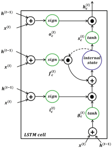
RNNs have various forms, the most fundamental of which are (1) one input to multiple outputs, (2) multiple outputs to one input, and (3) many inputs to many outputs. Some of their drawbacks include “vanishing gradients,” when input information passes through many layers, and then vanishes when reaching to the beginning or the end layer; and “exploding gradients,” where input information passes through many layers that end up with a large gradient when reaching to the beginning or the end layer. This presents issues in training RNNs, which creates more problems when long-term dependencies occur. LSTM models are a type of RNNs, whose memory architecture helps to accommodate inputs via long-term dependencies (capturing features and preserving information over long periods) (Ma et al. 2019). An LSTM model (Figure 2) is based on three gates: (1) the forget gate for decisions; (2) the output gate, where results are presented; and (3) the input gate, where information is added to the memory.

Figure 2. LSTM cell structure.

Source: Ma et al. (2019).

Fuzzy Logic Theorem

Fuzzy logic can be considered as decision-making tool and it is a subset of the intelligent system field. It is used in the simulation of non-linear behavior using the fuzzy logic framework. Despite its name, it is actually more of a precise logic for rational decisions in light of uncertainty (Singpurwalla and Booker 2004). As explained previously, fuzzy logic was originally proposed as a solution to handle uncertainty by approximation (Baatarchuluun, Sung, and Lee 2020). A fuzzy system includes a membership function, which can be of different curve shapes (trapezoidal, triangular, or Gaussian); the curve shows the connection between each input point and value between 0 and 1 (Sowlat et al. 2011).

Materials and Methods

The modeling stage requires combining data from various sources, in order to achieve an appropriate level of accuracy (Zayed and Abbod 2022a, 2022b). We took into consideration the data used and the domain (air quality), following the steps described below in order to obtain the final results.

Firstly, gas concentration was used as the output data for the Markov model. Any missing data were first processed with a moving mean for each gas, and then as a previous value, to back up any missing values for which the data was completed by the mean. The input data (wind speed, wind direction, temperature, and humidity) inputs were fed to the Markov model, which simulated the results.

The gas concentration results from the Markov model were fed to the DNN model (acting as the output). The inputs (i.e., the original inputs for the DNN model) were: day, month, year, hour, wind speed, wind direction, temperature and humidity. The final results were the outputs predicted after the running of the DNN model (Zayed and Abbod 2022a, 2022b).

Parameters Selection

A thorough literature review was done for input and output selection for studies of how air quality prediction has been undertaken by previous researchers, and it was found that a significant number used wind speed, wind direction, humidity, and temperature in different combinations, based on the studies’ setups. Furthermore, this study collected available data from the parameters available for selected locations in Jordan and England, as explained below. The selection of input and output was then performed based on the aims and objectives of this study. Most related studies performed prediction in isolation of the other gases factor, and this research aims to provide multivariate output predictions by having multiple outputs.

Data Sources, Collection, and Processing

Data was collected after a comprehensive review of the literature on the air-quality domain. This informed our view of the factors affecting gas concentrations in air, and these were selected as parameters for the models in this research. Accordingly, in this big data comparative study, data was selected in order to compare developed and developing cities for which sufficient data fulfilling the aim and objectives of the research were available and accessible. The data used in this research were collected from three different sources, as adumbrated below (Zayed and Abbod 2022a, 2022b).

First location: Marylebone Road, London

Source: Open data (United Kingdom):

https://www.londonair.org.uk/LondonAir/Default.aspx.

• Inputs: day, month, year, hour, humidity, temperature, wind speed, wind direction

• Output: CO (µg/m³) NO (µg/m³), NO2 (µg/m³), NOx (µg/m³), O3 (µg/m³), PM10 (µg/m³), SO2 (µg/m³)

• Size: 43824 data point

Second location: Greater Amman Municipality (GAM)

Source: Closed data (Jordan)

Data (from traffic locations) was collected from the Jordanian Ministry of Environment.

• Input: day, month, year, hour, humidity, temperature, wind speed, wind direction

• Output: PM10 (µg/m³), NO2 (ppb), CO (ppb), SO2 (ppb)

• Size: 26268 data point

Third location: Unspecified Italian city

Source: Open data (Italy)

UCI Machine Learning Repository: Air Quality Data Set

Italy data parameters:

• Date (DD/MM/YYYY)

• Time (HH.MM.SS)

• True hourly averaged concentration CO in mg/m³ (reference analyzer) PT08.S1 (tin oxide) hourly averaged sensor response (nominally CO targeted)

• True hourly averaged overall non-methanic hydrocarbons concentration in microg/m³ (reference analyzer)

• True hourly averaged Benzene concentration in µg/m³ (reference analyzer)

• PT08.S2 (titania) hourly averaged sensor response (nominally NMHC targeted)

• True hourly averaged NOx concentration in ppb (reference analyzer)

• PT08.S3 (tungsten oxide) hourly averaged sensor response (nominally NOx targeted)

• True hourly averaged NO2 concentration in microg/m³ (reference analyzer)

• PT08.S4 (tungsten oxide) hourly averaged sensor response (nominally NO2 targeted)

• PT08.S5 (indium oxide) hourly averaged sensor response (nominally O3 targeted)

• Temperature in °C

• Relative humidity (%)

• Absolute humidity

All data sets units for data sources, data collection and data processing are the same. Data were converted after prediction for the AQI representation purposes. There were four data phases: collection, processing, modeling, and obtaining of outputs. While optimal accuracy was the intended aim, challenges were presented by issues including data losses and data sparseness (issues of data collection); noisy and incomplete data (issues of data preprocessing); and accuracy and scalability (issues of data modeling). Some solutions to these issues were suggested by the literature (Zayed and Abbod 2022a, 2022b), including removing noise (by filtering data such as null). During the data check undertaken before the modeling phase, major data losses were found for temperature, wind speed, wind direction and humidity.

Accordingly, other data sources were provided: e-mails were sent to representatives of the areas listed above, who suggested using similar data from the nearest available area to the one selected (for instance, London City Airport was said to be “the nearest area to Marylebone Road”). The missing data was retrieved using R software (source) and the data was replaced (by checking where it was null or zero and replacing it with the City Airport value for the corresponding hour, where applicable) (Zayed and Abbod 2022a, 2022b).

Experimental Design Framework

The purpose of this research is to build a prediction model for next hour forecasting and to define measurable (quantifiable) data and compare different models for air quality prediction recommendations. Several machine learning regression methods have been used to compare results and model results using MATLAB R2020a software. Algorithms presented by reviewed studies were analyzed in the domain, and then experimenting top niche of them in an effort to develop a new and more time-efficient and accurate models to support air quality prediction.

Experiment Stages

1. Stage 1: Data collection

2. Stage 2: Data pre-processing

3. Sage 3: Data preparation

4. Stage 4: Models development

Models development phase 1

• NN (feed-forward backdrop)

• NN fitting

• NN time series (NARX)

Models development phase 2

• DNN

• Markov Chain

• Hybrid Model (DNN and Markov)

Stage 5: Models performance evaluation

Models

Models Development Phase 1

This research seeks to build a prediction model and define measurable (quantifiable) data set to a measurable index (i.e., the AQI). Several machine learning methods were used to compare and model results using MATLAB R2020a software in the initial stage using the fitting tool and time-series apps, as well as ANN – nntool.

Results were compared and the time-series app exhibited better results in all tested cases and scenarios for the same data set. After checking with several ANN models, DNN model was developed first based on the Jordanian data. Hyper parameters tuning was performed to the model until suitable accuracy was achieved. Then model was used for England data and gradual modifications were happening to achieve suitable accuracy. A Markov model was then developed independently for the Jordan and England data, and it was built to fulfil the data structure and the objectives of the experiment. After approaching sensible accuracy, a hybrid model took a huge part of the experiment, to have better accuracy than both developed models independently.

Models Development Phase 2

Deep-learning modeling architecture was built, using some of the methods and techniques discussed in this section. Due to the advantages of the DNN model in big-data prediction, many trials were performed, using tailored parameters to fit the data requirements, to produce appropriate accuracy for the predictions. The multivariate model improved the performance of the data from both Jordan and England. A DNN model with two LSTM layers was used as the first method of predicting air quality for the selected data (Zayed and Abbod 2022a, 2022b). A separate experiment was performed using Markov-chain modeling, and then hybrid modeling was developed, so that the test data was fed to the Markov model. This produced the required outputs and gave an indication of appropriate levels of accuracy (see Table 2).

By its nature, the Markov model requires data to be prepared in a certain way, so the Markov-switching regression was tailored to this particular research (Kim 1994) and was treated in a special way to fulfil the specific aims of the model. The initial input consisted of multiple inputs of eight parameters. When preparing to feed the Markov model with data, the data set was split randomly in a ratio of 0.8:0.1:0.1–0.8 for training, 0.1 for testing and 0.1 for validation. The data was then filled with movemean, as the first method, and the previous value, as the second method, to back up any missing values, for which the data were filled up using the mean. Indexing for both the input and output data was done in such a way as to treat each input and output as separated parameters. This procedure was based on previous trials, in which it was attempted to replace missing values on the run time using different methods.

The method described gave good results when it was applied to the data for both England and Jordan. This method of replacing the data was also suitable for this hourly data, as the first replacement of mean values through movemean method was aligned with the frequency of the data. The second method of replacement through previous value is also likely to be appropriate. Because of the nature of the data selected, there was a realized pattern of values, which was relatively close to each other’s readings on many occasions. This is because of the impact of weather conditions as a collective atmospheric effect, and the steep corresponding increase or decrease in values.

Movemean was chosen as the primary method of replacing missing cover values, as it can give near-average replacements. It should be noted here that the data contain negative temperature values, which were not manipulated, as they represent the reality of weather conditions and sub-zero temperatures, particularly in winter. The Markov model was based on several input models. Each input was represented by an ARIMA model, which was built using a number of variables: AR (auto regression coefficient), beta (regression coefficient); constant (mean); and variance (standard deviation). The AR variable for each input y was calculated using correlation function for each input and output, and then taking the mean as the result of the correlation (the value being used for each input ARIMA mode): the beta was a fixed value of 1 and the constant was a fixed value of zero.

The standard deviation changed according to each input value. An std function was used for each input: std (Input1), std (Input2), std (Input3), std (Input4), std (Input5), std (Input6), std (Input7) and std (Input8). A DTMC object (discrete-time Markov chain) was used for the switching-technique Markov-switching dynamic regression model msVAR object, which stored the parameter values of the model. The DTMC object took the P parameter as referred to the probability of the transition. When the output values stored in the Mdl variable were then simulated using the simulation function in MATLAB, which took the saved Mdl representing the input side, a number of observations (referring to the number of data rows used in the experiment) and the output were produced. A simulation object was used for each output, and it should be mentioned here that the output was named Training-Data in the code, so that TrainingData1 represented the value of Output1, Training-Data2 represented Output2, Training-Data3 represented output3 and TrainingData4 represented Output4.

The probability transition was created in eight different states, based on the eight input values. The assumption for the probability matrix was to produce an 8-by-8 matrix between zero and one, by generating a random number from a uniform distribution in range (0,1). All new outputs were represented using Training-Data, as all simulated outputs are stored in this variable. The transition probabilities linked each state to the next one; the earlier described model created a Markov-switching dynamic regression model which supported the dynamic behavior of the time series through the set of state transition probabilities. ARIMA and msVAR were used to create the dynamic regression model.

The DNN and Markov models were trained using the methods described above. Both trained models were saved appropriately, the resulted output of the DNN was fed to the Markov model as a new output and the values were predicted using the previously trained model parameters. The new output represented the predicted values for the hybrid model (both DNN and Markov). Data manipulation was performed in order to execute the hybrid model. This was done by using the output data of the validation model as the output for the first DNN model. The resulting values were then used as the output of the previously trained Markov model, as test data were used alongside other data in this experiment. A third source of data was considered to be external to the other data. This was used to predict the output, in order to validate the model and show how well it would perform with new data. The modeling results are presented in results section.

Considerations and Challenges

The study included a substantial number of trials to enhance the reliability of the findings. The experiment involved repeated thousands of trials to examine the stability and consistency of the observed effects; this is a lengthy study, and approximately 2 years of continuous trials were necessary for the practical work to attain the current proposed shape. The challenges encountered are as summarized below:

• Data complexity: the models consist of multivariate data (multi-inputs and multi-outputs). This added challenges to the work of data pre-processing and training time (for each trial the DNN model took approximately three and 2 days to run for data for England and Jordan, respectively).

• Model complexity: challenges in selecting a suitable algorithm for study were encountered, requiring a thorough literature review studying many elements and factors. Besides the overhead of DNN and the computational resources required, model hyper-tuning is a significant part of optimization research. It took quite a long time to run trials and find the optimal combination of suitable parameters for this study. Integrating two models to create hybrid model consisted of several steps, scenarios, and configurations to approach suitable results effectively aligned with the aims and the objectives of the study.

Results

England and Jordan Model Results (Models Phase 1)

Previous research on phase 1 model results presented NN methods, as shown in Table 1, indicating that NN-NARX outperformed other methods conducted; however, Zayed and Abbod (2022a, 2022b) stated that the nature of emissions and the complexity of some gases led to discovering other new methods (as described in the next section) that provide improved predictive performance and effectiveness as contribution to the air quality modeling field.

Table 1. Neural network modeling results.

Model type	Location	Accuracy	No. hidden units	Training Function
NN -FFB	Jordan	0.94	20	trainlm
NN -FFB	England	0.89	25	trainlm
NN-Fitting	Jordan	0.93	20	trainlm
NN-Fitting	England	0.88	25	trainlm
NN-NARX	Jordan	0.98	20	trainlm
NN-NARX	England	0.97	25	trainlm

Source: Zayed and Abbod (2022a, 2022b).

England and Jordan Model Results (Models Phase 2)

As Table 2 demonstrates, the accuracy of the hybrid models in the selected locations in England and Jordan is better than that of the DNN and Markov models. The hybrid models provided good accuracy in both experiments. Moreover, the performance of the models was validated using the new data. Improved accuracy was also noticed when the same hybrid models were used. This shows that they are preferable to the standalone models, in the light of the multivariate data from both England and Jordan. This study shows that combining two models supporting the time-series nature of air quality data has enhanced the experimental results. The first experiment was performed to obtain appropriate results for each individual model. The hybrid model was then applied to the experiment to achieve the required level of prediction accuracy.

Table 2. Modeling results: Jordan.

Model	England RMSE	Jordan RMSE
DNN	53.3712	77.7665
Markov	11.1347	15.6624
Hybrid (DNN and Markov)	9.8892	14.8770

Hybrid Model Validation

To validate the performance of the models, new data was selected from a data source that was not used in the experiment, in order to validate and evaluate the models and calculate the error for the models, using RMSE. The first stage of the validation was data preparation from the new source. Data were selected with similarities to the original data specifically to fulfil the requirements of the study, to ensure that the model would perform well with similar studies and data, and show that it was reliable. Data were selected from the Italian data source, which resembled the data used to build the models mentioned above.

After preparation of the input data, the data was partitioned to fit the number of rows selected for the test data. The new input data was then fed to the DNN model (after the previously saved DNN model results were loaded to the MATLAB workspace). A run of the prediction was then performed with the current settings, but without retraining the DNN (the pre-saved model set-up was used). Finally, the new predicted result was fed to the Markov model (after the previously saved Markov model results were loaded to the MATLAB workspace), and the results from this run were considered for the validation of the hybrid modeling results.

A new source of data was used to validate the Jordan modeling: KHG location data, provided by the Jordanian Ministry of the Environment. Firstly, the DNN and Markov models were trained and each set of results saved separately. The externally sourced test data was predicted (fed) first to the DNN and then to the Markov (see Tables 3 and 4). The results were validated using the new Italian data. The output was used to perform a new DNN run, using this data source. As Table 2 shows, the accuracy of the hybrid models in both England and Jordan was better than that of the DNN and Markov models. The hybrid model showed good accuracy in both experiments. Its performance was validated using new data, while it showed greater accuracy, compared to the standalone models.

Table 3. Modeling validation (new data source from Italy): England modeling.

Model	England RMSE	Italy RMSE
DNN	57.4937	113.3896
Markov	10.48610	18.7021
Hybrid (DNN and Markov)	7.8666	15.2777

Table 4. Performance evaluation metrics for the hybrid models.

MAE	R	Model
8.2426	0.9966	Hybrid (DNN and Markov) – Jordan
14.6901	0.9986	Hybrid (DNN and Markov) – England

Discussion

Air Quality Index

AQI (England)

The AQI for England was produced using the following method:

• Firstly, the most accurate output was selected from the predictive modeling.

• The units were converted for some gases to comply with the requirements of the EPA

• The maximum value of each gas was determined using loop and max functions (showing which gas had the highest value at the specified point in time).

• The AQI was found for each gas concentration at the specified point of time, according to the EPA standards (representing the AQI levels).

The conversion units can be seen in Table 5.

Table 5. Conversion of units for emissions.

Unit of emission	EPA unit	Conversion
CO (mg/m^3)	mg/m^3	24.45*CO concentration/28.01
NO (μg/m^3)	μg/m^3	24.45* NO concentration/30
NO2 (μg/m^3)	μg/m^3	24.45* NO2 concentration/46.006
NOX (μg/m^3)	μg/m^3	24.45*NOX concentration 46.006
O3 (μg/m^3)	μg/m^3	24.45*O3 concentration/48.0
SO2 (ug/m^3)	μg/m^3	24.45*SO2 concentration/64.06

AQI (Jordan)

The AQI for Jordan was produced using the following method:

• Firstly, outputs were selected from the predictive modeling.

• The units were converted for some gases to comply with the requirements of the selected AQI standard (US EPA 2016). CO was the only gas reading in the Jordan data that needed unit conversion (from ppb to ppm, dividing the values by 1000).

• The maximum value of the gases was found using the loop and max functions (to determine which gas had the highest value at that point in time).

• The AQI could then be found for each gas concentration at the specified point in time, following the EPA standards (representing the AQI levels) (US EPA 2016).

PM did not require any conversion, as all the units for the collected data matched the relevant EPA unit.

Neuro-fuzzy Logic (Representing the AQI)

Neuro-fuzzy logic was used in this study to represent the AQI for the predicted measurements.

• The data inputs (for fuzzy logic) for England were: Input1 (CO), Input2 (NO), Input3 (NO₂), Input4 (NO_x), Input5 (O₃), Input6 (PM₁₀) and Input7 (SO₂).

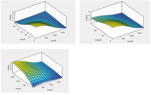
• The data inputs (for fuzzy logic) for Jordan were: Input1 (PM₁₀), Input2 (NO₂), Input3 (CO) and Input4 (SO₂)

In this neuro-fuzzy logic model, the outputs were considered to be inputs for the model. Firstly, for the training data, the initial outputs represented the inputs, while the outputs represented the AQI assigned to each value, based on the US EPA (2016) levels. Secondly, for the testing data, the predicted outputs represented the inputs, while the outputs represented the AQI assigned to each value, based on the US EPA levels. For the model setup, a Gaussian (gaussmf) was used as the input MF (membership function) type and a linear function was selected for the output MF (membership function) type. Two membership functions were used for each variable (see Figures 3 and 4).

Figure 3. Neuro-fuzzy logic representing the air quality index data for England, with 128 rules.

Note. Sample representation of first input (CO) and all other inputs. Input1 (CO), Input2 (NO), Input3 (NO2), Input4 (NOx), Input5 (O3), Input6 (PM10), and Input7 (SO2).

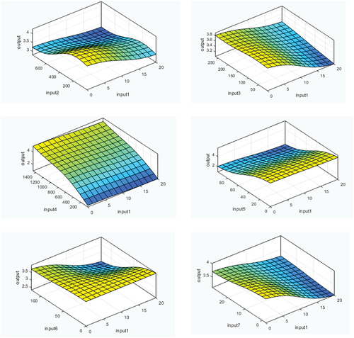
Figure 4. Neuro-fuzzy logic representing the air quality index data for Jordan, with 16 rules.

Note. Sample representation of the first input3 (CO) and all other inputs. Input1 (PM10), Input2 (NO2), Input3 (CO) and Input4 (SO2).

For the purposes of illustration, CO was selected to check the AQI representation against all other inputs. The control surface in Figure 3 shows the overall mapping between (Inputs) and (Outputs). It can be inferred that the output in this case (CO) is at highest value relatively when Input4 (NOx) and Input5 (O3) are high, which is almost AQI (4) on a scale from 1 to 7 for the AQI. Further, it is clear that Input6 (PM₁₀) and Input7 (SO₂) are influencing the AQI levels. It can be concluded that different gases with different concentrations affect the output level of gases in light of weather conditions such as wind speed, wind direction, temperature, and humidity.

Figure 5. Representation of neuro-fuzzy logic structure (data from Jordan).

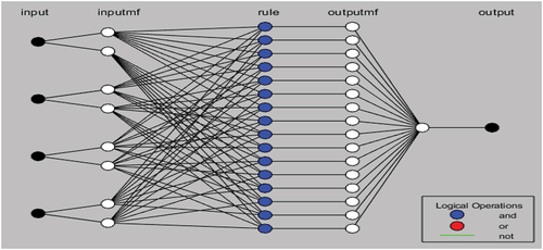
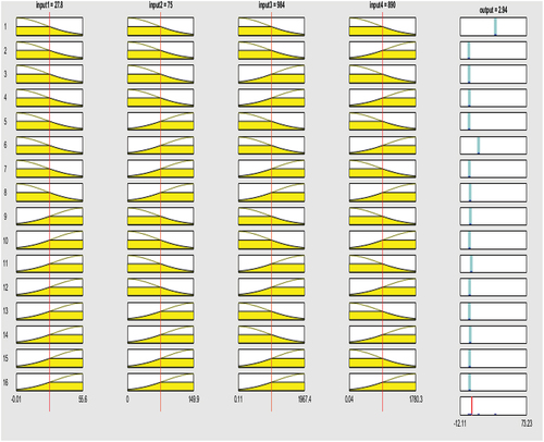
As can be seen from Figure 4, Input4 (SO2) is greatly impacting the pollution level with the highest value for AQI (5) on a scale from 1 to 7. Input 2 (NO2) has a moderate influence on the AQI levels. Figure 5 shows neuro-fuzzy logic structure and Figure 6 represents neuro-fuzzy rules for the Jordan data as an example, and it is used to evaluate the created rules to validate the fuzzy model.

Figure 6. Representation of neuro-fuzzy logic rules (data from Jordan).

Concluding Remarks

After completing both the Markov Chain and DNN modeling, the results were assessed and reported. As the aim of this research was to increase accuracy and obtain more reliable results, a hybrid model was proposed by the researchers, to ensure better interpretation of the data and more appropriate results. Many experimental trials were conducted in order to achieve the best scenario possible with the data available for this study. The DNN-Markov model was determined to be the best hybrid model, for data from both England and Jordan.

The authors of this research argue that an AQI is an effective method of measuring healthy levels of the air we breathe every day, and so a predictive framework for air quality indices is presented in this study. At times of high toxic pollutant exposure, the researchers have introduced methods of predicting hourly emission concentrations and producing related AQI levels as a control system for vulnerable areas.

The study conducted several methods in an effort to contribute a new and efficient approach to predict AQI for the next hour; DNN-Markov approach was selected as the model proved performance through validation which holds a promising potential for efficiency as well as of using simple linear model to backup for the complexity and losses that could occur of the DNN model which is a boost for performance.

Contributions, Limitations, and Future Research Directions

In addition to developing a model that achieved accuracy rates of approximately RMSE 7.86 and 15.27 for studied locations in England and Jordan (respectively), this study makes a set of contributions including the following:

• Hourly prediction model has been proposed

• Multivariate input and output models that support the complexity of air quality prediction.

• Hybrid modeling methods (Markov and DNN) were combined.

• AQI representation.

This study has industrial significance, as air pollution has affected many aspects of life, the most egregious of which is health, with increased prevalence of respiratory irritation issues (Coelho et al. 2021). The first air quality index was developed by the USAEPA as a response to the major economic, health, and environmental consequences of industrial activities (Bishoi, Prakash, and Jain 2009). The USAEPA standard is adopted in this study to represent air quality levels. The authors of this research propose the development of a neuro-fuzzy-logic system to support the boundary areas of the Air Quality Index (AQI) as a further enhancement for representing air quality levels. However, this research was limited by data availability, which restricted the study to the selected features and specific emission gases for different location studies. Further developmental research is required to address literature gaps in the field.

Disclosure Statement

No potential conflict of interest was reported by the author(s).

Data Availability Statement

The data that support the findings of this study are available from the corresponding author, M.A., upon reasonable request.

Additional information

Funding

The work was supported by the Brunel University London.

References

- Alnawaiseh, N. A., and J. H. Hashim. 2014. Respiratory symptoms from particulate air pollution related to vehicle traffic in Amman, Jordan. European Journal of Scientific Research 120 (4):550–24.
- Ameer, S., M. A. Shah, A. Khan, H. Song, C. Maple, S. U. Islam, and M. N. Asghar. 2019. Comparative analysis of machine learning techniques for predicting air quality in smart cities. Institute of Electrical and Electronics Engineers Access 7:128325–38. doi:10.1109/ACCESS.2019.2925082.
- Baatarchuluun, K., Y.-S. Sung, and M. Lee. 2020. Air pollution prediction model using artificial neural network and fuzzy theory. International Journal of Internet, Broadcasting and Communication 12 (3):149–55. doi:10.7236/IJIBC.2020.12.3.149.
- Barrera-Animas, A. Y., L. O. Oyedele, M. Bilal, T. D. Akinosho, J. M. D. Delgado, and L. A. Akanbi. 2022. Rainfall prediction: A comparative analysis of modern machine learning algorithms for time-series forecasting. Machine Learning with Applications 7:100204. doi:10.1016/j.mlwa.2021.100204.
- Bishoi, B., A. Prakash, and V. K. Jain. 2009. A comparative study of air quality index based on factor analysis and US-EPA methods for an urban environment. Aerosol and Air Quality Research 9 (1):1–17. doi:10.4209/aaqr.2008.02.0007.
- Cheng, W. L., Y. S. Chen, J. Zhang, T. J. Lyons, J. L. Pai, and S. H. Chang. 2007. Comparison of the Revised Air Quality Index with the PSI and AQI indices. Science of the Total Environment 382 (2–3):191–98. doi:10.1016/j.scitotenv.2007.04.036.
- Coelho, S., S. Rafael, D. Lopes, A. I. Miranda, and J. Ferreira. 2021. How changing climate may influence air pollution control strategies for 2030? Science of the Total Environment 758:143911. doi:10.1016/j.scitotenv.2020.143911.
- Devasekhar, V., and P. Natarajan. 2023. Prediction of air quality and pollution using statistical methods and machine learning techniques. International Journal of Advanced Computer Science and Applications 14 (4):927–37. doi:10.14569/IJACSA.2023.01404103.
- Iain, L., and W. Z. MacDonald. 2016. Hidden Markov and other models for discrete- valued time series: An introduction using R. 2nd ed. London: Chapman & Hall/CRC.
- Kaur, G., and J. Gao. 2018. Air quality prediction: Big data and machine learning approaches component testing. International Journal of Environmental Science and Development 9 (1):8–16. doi:10.18178/ijesd.2018.9.1.1066.
- Kaur, M., D. Singh, M. Y. Jabarulla, V. Kumar, J. Kang, and H.-N. Lee. 2023. Computational deep air quality prediction techniques: A systematic review. Artificial Intelligence Review 56 (S2):2053–98. doi:10.1007/s10462-023-10570-9.
- Kemeny, J. G., and J. L. Snell. 1983. Finite Markov chains: With a new appendix “Generalization of a Fundamental Matrix”. Dordrecht: Springer.
- Kim, C. J. 1994. Dynamic linear models with Markov-switching. Journal of Econometrics 60 (1–2):1–22. doi:10.1016/0304-4076(94)90036-1.
- Liu, X., C. Guo, Y. Wu, C. Huang, K. Lu, Y. Zhang, L. Duan, M. Cheng, F. Chai, F. Mei, et al. 2023. Evaluating cost and benefit of air pollution control policies in China: A systematic review. Journal of Environmental Sciences 123:140–55. doi:10.1016/j.jes.2022.02.043.
- Ma, J., J. C. P. Cheng, C. Lin, Y. Tan, and J. Zhang. 2019. Improving air quality prediction accuracy at larger temporal resolutions using deep learning and transfer learning techniques. Atmospheric Environment 214:116885. doi:10.1016/j.atmosenv.2019.116885.
- Mandal, T. K., and A. Gorai. 2014. Air quality indices: A literature review. Journal of Environmental Science & Engineering 56 (3):357–62.
- Masih, A. 2019. Machine learning algorithms in air quality modeling. Global Journal of Environmental Science and Management 5 (4):515–34. doi:10.22034/gjesm.2019.04.10.
- Méndez, M., M. G. Merayo, and M. Núñez. 2023. Machine learning algorithms to forecast air quality: A survey. Artificial Intelligence Review 56 (9):10031–66. doi:10.1007/s10462-023-10424-4.
- Monteiro, A., M. Vieira, C. Gama, and A. I. Miranda. 2017. Towards an improved air quality index. Air Quality, Atmosphere and Health 10 (4):447–55. doi:10.1007/s11869-016-0435-y.
- Niharika, V. M., and P. A. Rao. 2014. Survey on air quality forecasting techniques. International Journal of Computer Science and Information Technologies 5 (1):103–07.
- Niska, H., T. Hiltunen, A. Karppinen, J. Ruuskanen, and M. Kolehmainen. 2004. Evolving the neural network model for forecasting air pollution time series. Engineering Applications of Artificial Intelligence 17 (2):159–67. doi:10.1016/j.engappai.2004.02.002.
- Shrestha, A., and A. Mahmood. 2019. Review of deep learning algorithms and architectures. Institute of Electrical and Electronics Engineers Access 7:53040–65. doi:10.1109/ACCESS.2019.2912200.
- Siami-Namini, S., N. Tavakoli, and A. S. Namin. 2019. The performance of LSTM and BiLSTM in forecasting time series. In 2019 IEEE International Conference on Big Data 2019, 3285–92. doi:10.1109/BigData47090.2019.9005997.
- Singpurwalla, N. D., and J. M. Booker. 2004. Membership functions and probability measures of fuzzy sets. Journal of the American Statistical Association 99 (467):867–77. doi:10.1198/016214504000001196.
- Sowlat, M. H., H. Gharibi, M. Yunesian, M. Tayefeh Mahmoudi, and S. Lotfi. 2011. A novel, fuzzy-based air quality index (FAQI) for air quality assessment. Atmospheric Environment 45 (12):2050–59. doi:10.1016/j.atmosenv.2011.01.060.
- Staudemeyer, R. C., and E. R. Morris. 2019. Understanding LSTM: A tutorial into long short-term memory recurrent neural networks. arXiv. September 9. doi:10.48550/arXiv.1909.09586.
- Tealab, A. 2018. Time series forecasting using artificial neural networks methodologies: A systematic review. Future Computing and Informatics Journal 3 (2):334–40. doi:10.1016/j.fcij.2018.10.003.
- Tripathi, K., and P. Pathak. 2021. Deep learning techniques for air pollution. In IEEE 2021 International Conference on Computing, Communication, and Intelligent Systems 2021, ii:1013–20. doi:10.1109/ICCCIS51004.2021.9397130.
- US EPA. 2016. Patient exposure and the air quality index. Last Modified November 20, 2023. Accessed December 10, 2023. https://www.epa.gov/ozone-pollution-and-your-patients-health/patient-exposure-and-air-quality-index.
- van den Elshout, S., K. Léger, and F. Nussio. 2008. Comparing urban air quality in Europe in real time: A review of existing air quality indices and the proposal of a common alternative. Environment International 34 (5):720–26. doi:10.1016/j.envint.2007.12.011.
- Zayed, R., and M. Abbod. 2022a. Big Data AI system for air quality prediction. Data Science and Applications 4 (2):5–10.
- Zayed, R., and M. Abbod. 2022b. Hybrid intelligent modelling for air quality prediction deep learning and Markov chain unconventional framework. International Journal of Simulation Systems, Science & Technology 23 (1):3.1–6. doi:10.5013/IJSSST.a.23.01.03.
- Zheng, Y., X. Yi, M. Li, R. Li, Z. Shan, E. Chang, and T. Li. 2015. Forecasting fine-grained air quality based on Big Data. In Proceedings of the 21th ACM SIGKDD International Conference on Knowledge Discovery and Data Mining KDD’, vol. 15, 2267–76. doi:10.1145/2783258.2788573.