The impact of the thermostats on the non-equilibrium computer simulations of the interfacial thermal conductance

ABSTRACT

Non-equilibrium molecular dynamics simulations have expanded our ability to investigate interfacial thermal transport and quantify the interfacial thermal conductance (ITC) across solid and fluid interfaces. NEMD studies have highlighted the importance of interfacial degrees of freedom and the need to include effects beyond traditional theoretical methods that rely on bulk properties. NEMD simulations often use explicit hot and cold thermostats to set up thermal gradients. We analyse here the impact of the thermostat on the calculated ITC of the gold-water interface. We employ a polarisable model for gold based on Drude oscillators. We show that the ‘local’ Langevin thermostat modifies the vibrational density of states of the polarisable solid, resulting in ITCs that depend very strongly on the damping constant of the thermostat. We report an increase of the ITC of up to 40% for short damping times. Damping times longer than the characteristic heat flux relaxation time of the solid lead to converging ITCs. In contrast, the ITCs obtained with global canonical velocity rescale thermostats are independent of the damping time but lead to a break of equipartition for Drude particles. Setting individual thermostats for the core and shell sites in the Drude particle solves this problem.

KEYWORDS:

• Interfacial thermal conductance
• non-equilibrium molecular dynamics
• gold-water interface
• polarisation
• thermostats

1. Introduction

The Interfacial Thermal Conductance (ITC), $G_K$, or its inverse, the Kapitza resistance [1,2], determines the temperature ‘jump’ across an interface and the timescale for the heat transfer across the interface. The quantification of the thermal conductance has attracted increasing interest, given its relevance in heat dissipation processes in microelectronics and nanomaterials [3]. Theoretical calculations of the ITC rely on the bulk properties of the materials in contact [2]. However, experimental studies of surfaces coated with self-assembled monolayers showed that local changes in the monolayers' chemical composition result in significant changes of the thermal conductance [4], highlighting the need to include interfacial properties explicitly.

Non-Equilibrium Molecular Dynamics simulations (NEMD) [5] provide a powerful approach to calculate the ITC, $G_K=J_q/\mathrm{\Delta }T$, as the heat flux $J_q$ and the temperature ‘jump’, $\mathrm{\Delta }T$, can be computed easily. NEMD has been used to study aqueous interfaces with solids [6,7], liquids [8], solid surfaces coated with self-assembled monolayers [9]. Further, simulations provided insight into the dependence of the ITC with interfacial curvature and intermolecular interactions [10–14]. Generally, the ITC increases with interfacial curvature and with substrate-liquid interactions. An attempt to rationalise experimental measurements of nanoparticle-fluid ITC was reported recently using NEMD techniques [11]. Further, NEMD simulations, in combination with so-called intrinsic interfacial methods, were used to identify the interfacial regions responsible for the ITC in liquid-vapour interfaces [15].

The NEMD approach to calculate ITCs is easy to implement. The stationary version of the method requires the use of hot and cold thermostats to set up the thermal gradient and the corresponding heat flux. The thermostats are applied to different regions in the simulation box, while the dynamics of the atoms or molecules in the non-thermostatted regions evolve following Newtonian dynamics. Recent work has discussed the caveats of using the Stationary NEMD (SNEMD) approach to calculate the thermal conductivity of bulk solids [16–19]. The main problem in these computations arises from imposing an artificial cutoff, the distance between hot and cold thermostats, to the phonons' mean free path. This cutoff leads to thermal conductivities that are lower than those computed in the bulk solid. In contrast, the calculation of the thermal conductivity of fluids with SNEMD does not suffer from significant cutoff effects since the collisions between close neighbours dominated the heat transport mechanism. Hence, the characteristic mean free path for heat transport is of the order of a molecular diameter, much shorter than the typical distance between the thermostats in the SNEMD approach.

In addition to the size effects discussed above, the type of local thermostats to set hot and cold regions influences the heat conduction in solids. Recent NEMD simulations of graphene multilayers [20] showed that the ‘local’ Langevin thermostat provides a better approach than ‘global’ thermostats, such as Nosé-Hoover, which lead to artificial thermal rectification effects. The Langevin thermostat performed better in NEMD simulations of molecular liquids, too, particularly in the equilibration of the fast degrees of freedom, such as intramolecular vibrations [21]. However, simulation studies have also uncovered issues associated with the Langevin thermostat. The vibrational density of states (VDOS) of silicon became smoother and broader than the VDOS obtained without that thermostat [22].

Despite several studies devoted to bulk systems, the impact of thermostatting on the ITC has not been investigated extensively. Thermostatting is important in ITC problems since these often involve solids in contact with liquids. Recent studies of solid-solid and solid-liquid interfaces of atomistic solids and fluids showed that Langevin and dissipative particle dynamics (DPD) thermostats might lead to spurious thermal resistances [23].

In this work, we use NEMD simulations to investigate the impact of thermostatting on the interfacial thermal conductance of the gold-water interface. Gold is modelled as a polarisable solid using a Drude oscillator model introduced recently [24]. We show that the ITC depends significantly on the time constant used to set the Langevin thermostat. Short time constants lead to large over-estimations of the thermal conductance (up to 40% higher), and lack of conservation of the energy exchanged at hot and cold thermostats. Advancing the discussion below, we find that short damping times prevent the full relaxation of the heat flux correlations. The VDOS features significant changes with respect to the unthermostatted case, hence affecting the simulated ITC. Increasing the time constant to times longer than the characteristic relaxation time of the heat flux correlation solves this problem.

The velocity rescale thermostat [25] provides a robust approach to perform simulations of ITC since the computed ITCs are essentially independent of the time constant used for the thermostat. However, for polarisable solids modelled with Drude oscillators, we observe a breakdown of the equipartition between the core and shell sites, and the two sites feature different temperatures. We propose an approach to resolve this problem by applying velocity-rescale thermostats individually to the two sites in the Drude oscillator. The effects discussed in our work are general and relevant in non-equilibrium simulations of molecular systems that include explicit vibrational degrees of freedom.

2. Methodology

We performed non-equilibrium molecular dynamics simulations by heating the gold slab and cooling a water region at a distance of $\sim 22$ Å from the interface ($|x|>40$ Å). The water density in the cold thermostatting region was ${\rho }_m=1.0{\mathrm{g}/\mathrm{cm}}^3$, and the average density of water in the box ${\rho }_m=1.01{\mathrm{g}/\mathrm{cm}}^3$. The gold slab, with lattice parameter $a=4.078$ Å consisted of 15, 10 and 10 atomic layers in the x, y and z direction, respectively (dimensions of $35.32\times 28.84\times 24.97$ Å${}^3$). The simulation cell size was set to $(L_x\times L_y\times L_z)=113.06\times 28.84\times 24.97$ Å${}^3$). The liquid was in contact with the (111) plane of gold, with the interface located in the yz plane. We performed simulations using the velocity-Verlet integrator with several thermostatting approaches. In one set of simulations, we employed the Langevin thermostat [26] for the gold atoms and the canonical velocity rescaling thermostat (CSVR) [25] for water. In the second set of simulations, we used the CSVR thermostat for both gold and water. We tested a range of time constants from 0.1 ps to 2.5 ps. The centre of mass velocity of the water molecules and the gold slab was reset every timestep. The temperature of the hot and cold regions was 350 K and 300 K, respectively. 10–15 independent replicas were pre-equilibrated for 100 ps, and the data was sampled for 400 ps.

We used a polarisable model for gold introduced recently [24], which is based on a Drude oscillator approach, consisting of a core-shell pair for each gold atom. The core-shell pairs are bonded through a harmonic potential of the form: (1) $U_{bonded}=K(r_{ij}-r_0{)}^2,$(1) where $K=50{\mathrm{kcalmol}}^{-1}$ Å${}^{-2}$ is the harmonic spring constant and $r_0=0$ Å is the equilibrium distance, i.e. the position of the core atom. The non-bonded pair interaction is given by: (2) $U_{non-bonded}=\frac{q_i{q}_j}{4\pi {ϵ}_0{r}_{ij}}+4{ϵ}_{ij}[{\left(\frac{{\sigma }_{ij}}{r_{ij}}\right)}^{12}-{\left(\frac{{\sigma }_{ij}}{r_{ij}}\right)}^6],$(2) where ${ϵ}_0$ is the vacuum permittivity, $q_i,q_j$ are the charges of species i and j, respectively, $r_{ij}$ is the interparticle distance, and ${ϵ}_{ij}$ and ${\sigma }_{ij}$ are the Lennard-Jones coefficients for the pair interaction. We excluded the non-bonded interaction between core-shell particles belonging to the same gold atom. The van der Waals and real-space electrostatic interactions cutoff was 12 Å. The electrostatic interactions were computed with the particle-particle particle-mesh solver with a relative error of ${10}^{-5}$.

The water molecules were modelled using the rigid SPC/E model [27] (bond distance $r_{OH}=1$ Å and angle ${\theta }_{HOH}={109.47}^{\circ }$, respectively). Bond lengths and angles were kept constant during the simulation using the SHAKE algorithm [28]. The Lennard-Jones interactions parameters between the gold atoms and the water molecules were obtained using combination rules, ${ϵ}_{ij}=\sqrt{{ϵ}_i{ϵ}_j}$ and ${\sigma }_{ij}=\sqrt{{\sigma }_i{\sigma }_j}$. Table 1 collects the parameters for the non-bonded interactions .

Table 1. Simulation parameters used in this work for gold and water.

Non-bonded parameters	ϵ [kcal mol${}^{-1}$]	σ [Å]	q [e]	m (g/mol)
Au${}_c$	3.50	2.6246	+1.0	195.967
Au${}_s$	0.20	2.6246	−1.0	1.00
O	0.15535	3.166	−0.8476	15.9994
H	0.0	0.0	+0.4238	1.00794

Note: Au${}_c$ and Au${}_s$ represent the core and shell sites defining the gold atoms.

The temperature profiles needed to compute the temperature ‘jump’ were calculated by dividing the simulation box into subvolumes of thickness 2.35 Å, and using the equipartition principle.

2.1. Thermostats

In this section, we introduce the thermostats used throughout this work. Both Langevin and CSVR thermostats were applied to the gold slab, while only the CSVR thermostat was applied to water. A key difference between these two thermostats is that the Langevin thermostat acts on each particle (a local thermostat), while the CSVR thermostat rescales the velocities based on the kinetic energy of the target group of atoms (a global thermostat).

2.1.1. Langevin thermostat

The Langevin thermostat is based on the numerical solution of the Langevin equation of motion, which can be written as [29]: (3) $m_i\ddot{{\mathbf{r}}_{\mathbf{i}}}=-\mathrm{\nabla }U({\mathbf{r}}_{\mathbf{i}}\mathbf{,}\mathbf{R})-{\gamma }_i\dot{{\mathbf{r}}_{\mathbf{i}}}+\sqrt{2\gamma k_{B}T}F(t)$(3) where $m_i$ is the mass of particle i, U is the potential energy of particle i with coordinates ${\mathbf{r}}_{\mathbf{i}}$ in the field of all the other particles with coordinates $\mathbf{R}$. γ is the friction coefficient and $F(t)$ is a stochastic term with mean zero, $⟨F(t)⟩$ = 0, and a correlation given by a delta function, $⟨F(t)F(t^{\prime })⟩=\delta (t-t^{\prime })$. The friction coefficient, γ, is written in terms of a damping time, ${\tau }_D$, as ${\gamma }_i=m_i/{\tau }_D$. The equations of motion thus correspond to a fluid coupled to a heat bath, with the inverse of ${\tau }_D$ representing the strength of the coupling.

A practical implementation for the solution of Equation (3(3) $m_i\ddot{{\mathbf{r}}_{\mathbf{i}}}=-\mathrm{\nabla }U({\mathbf{r}}_{\mathbf{i}}\mathbf{,}\mathbf{R})-{\gamma }_i\dot{{\mathbf{r}}_{\mathbf{i}}}+\sqrt{2\gamma k_{B}T}F(t)$(3) ) consists on taking the stochastic force as random pulses sampled from a Gaussian distribution with standard deviation$\sqrt{2\gamma k_{B}T/\delta t}$, acting over a time period $[t-\delta t/2,t+\delta t/2]$, where $\delta t$ is the timestep of the numerical solver [30,31]. As discussed by Dunweg and Paul [26], taking a uniform distribution (instead of a Gaussian distribution) for the randomisation of the stochastic forces, results in a similar convergence of dynamical properties, in particular, mean first exit time of a particle during diffusive dynamics. We used the implementation in LAMMPS [32] (fix langevin) to solve the equations of motion.

We also performed additional simulation using the Grønbech-Jensen and Farago implementation of the Langevin thermostat [31] (fix langevin/gjf), which allows the use of longer time steps preserving the stability of the integration of the equations of motion.

2.1.2. Canonical velocity rescaling

A simple velocity rescaling thermostat [33] relies on rescaling the atomic velocities by a factor $\alpha =\sqrt{K_t/K_c}$, where $K_t$ and $K_c$ are the target and current kinetic energies of the system. As discussed by Bussi and coworkers [25], this rescaling algorithm does not sample the canonical distribution. Instead, the target kinetic energy must be sampled from a canonical distribution, such that the probability $P(K_t)\propto K_t^{N_f/2-1}\exp (-\beta K_t)$, where $N_f$ is the number of degrees of freedom in the system and $1/\beta =k_{B}T$. To control the strength of the thermostat, the authors introduced a coupling with a stochastic term characterised by a time constant (${\tau }_D$). Larger values of damping constant result in weaker coupling with the heat bath. For our computations, we used the default implementation in LAMMPS (fix temp/csvr).

Simple velocity rescaling leads to the ‘flying ice-cube effect’ [34–36], which leads to transfer of energy from fast to slow degrees of freedom, with an accumulation of kinetic energy in translational and rotational motions. A recent work showed the lack of flying ice-cube effect in a system of harmonically-bonded diatomic molecules (ethane) thermalised with the CSVR thermostat [36].

2.2. Calculation of heat flux correlation function and relaxation time

We calculated the heat flux autocorrelation function (HFACF) to obtain the relaxation time of the heat flux in the gold slab. The microscopic definition of the heat flux is given by Irving and Kirkwood [37], (4) ${\mathbf{J}}_q=\frac{1}{V}\sum _i{E}_i{\mathbf{v}}_i+\frac{1}{2V}\sum _{i<j}({\mathbf{f}}_{ij}\cdot ({\mathbf{v}}_i+{\mathbf{v}}_j){\mathbf{r}}_{ij})$(4) where the first term represents the contribution of the internal energy internal energy, $E_i$, of atom i with velocity ${\mathbf{v}}_i$ in volume V, to the heat flux. The second term in the equation above takes into account the collisional contribution to the heat flux. ${\mathbf{f}}_{ij}$ is the force between particles i and j at the distance ${\mathbf{r}}_{ij}$. 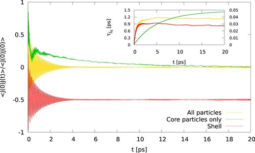The heat flux relaxation is given by the HFACF, (5) ${\tau }_{J_q}={\int }_0^{t_{max}}\frac{⟨{\mathbf{J}}_q(t^{\prime })\cdot {\mathbf{J}}_q(0)⟩}{⟨{\mathbf{J}}_q(0)\cdot {\mathbf{J}}_q(0)⟩}\mathrm{d}{t}^{\prime }$(5) where $t_{max}$ is the maximum integration time used to calculate ${\tau }_{J_q}$, chosen to ensure the correlation function decays to zero, and the corresponding integral features a well defined plateau. Figure 1 shows examples of the correlation functions and the corresponding running integrals. The relaxation time was obtained using a bulk gold crystal equilibrated at 300 K. The simulations were performed in the (NVE) ensemble.

Figure 1. (Colour online) Normalised heat flux correlation function of gold, considering all the atoms, core and shell particles (yellow), core particles only (green), or shell paricles only (red, shifted by -0.5). The inset shows the integrals given by Equation (5(5) ${\tau }_{J_q}={\int }_0^{t_{max}}\frac{⟨{\mathbf{J}}_q(t^{\prime })\cdot {\mathbf{J}}_q(0)⟩}{⟨{\mathbf{J}}_q(0)\cdot {\mathbf{J}}_q(0)⟩}\mathrm{d}{t}^{\prime }$(5) ). The dashed lines correspond to the secondary y-axis. The relaxation times are 0.027 ps, 0.037 ps, 1.42 ps, for shell particles, all particles and core particles, respectively.

2.3. Vibrational density of states

The vibrational spectra of the interfacial region was obtained by calculating the Fourier transform of the velocity autocorrelation function: (6) $D_{\alpha ,\xi }(\omega )={\int }_0^{\mathrm{\infty }}\frac{⟨v_{\alpha ,\xi }(0)v_{\alpha ,\xi }(t)⟩}{⟨v_{\alpha ,\xi }(0)v_{\alpha ,\xi }(0)⟩}\exp (-2\pi i\omega t)\mathrm{d}t$(6) where $⟨v_{\alpha ,\xi }(0)v_{\alpha ,\xi }(t)⟩$ is the velocity autocorrelation function of species α and component ξ, parallel (z,y) or perpendicular (x) to the interface plane. The frequency, ω, wavenumber, $\tilde{\nu }$, and wavelength, λ, are related via $\tilde{\nu }=\omega /c=1/\lambda$, where c is the speed of light. For the water molecules, the interfacial density of states, $D(\omega )$ included the atoms located in the first solvation layer in contact with gold. These atoms were followed for up to 4 ps, which defines the maximum correlation time for $⟨v(0)v(t)⟩$. 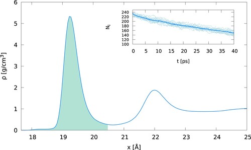After 4 ps, ∼10% of the initial water molecules left the interfacial region. Hence, after this time, we updated the list of molecules used to calculate D(ω). Figure 2 shows the density profile of water as a function of the distance to the gold surface, showing the definition of the interfacial region used in our computations.

Figure 2. (Colour online) Interfacial density profile of water as a function to the distance to the gold surface. The green-shaded area represents the region used to select water molecular for the calculation of the interfacial vibrational density of states. The inset shows the number of atoms (hydrogens and oxygens) that were initially in the interfacial region, and that stay in that region after time t. After 4 ps (the correlation time for Equation (6(6) $D_{\alpha ,\xi }(\omega )={\int }_0^{\mathrm{\infty }}\frac{⟨v_{\alpha ,\xi }(0)v_{\alpha ,\xi }(t)⟩}{⟨v_{\alpha ,\xi }(0)v_{\alpha ,\xi }(0)⟩}\exp (-2\pi i\omega t)\mathrm{d}t$(6) )), ∼90% of the original water molecules remain in the interfacial region. The full line corresponds to the average of 10 individual trajectories (shown by the dotted lines light blue).

3. Results and discussion

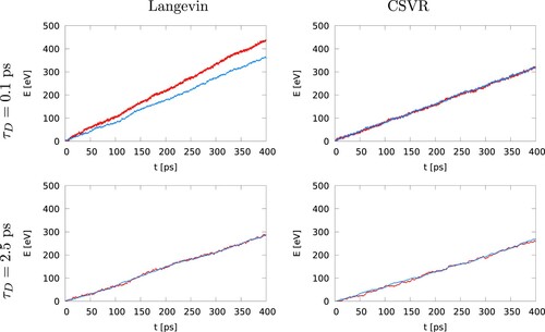
Figure 3 presents representative results for the energy exchanged at the hot and cold thermostats using both Langevin and the canonical velocity rescaling thermostats (CSVR). The damping times used for the Langevin thermostat have a significant impact on energy conservation. For short damping times, ${\tau }_D=0.1\mathrm{ps}$, the energies exchanged in the hot and cold region diverge over time. The lack of energy conservation decreases significantly by increasing the damping time to 2.5 ps. In this case, the difference between the energy exchanged in hot and cold thermostats is less than 0.01 eV/ps (vs 0.17 eV/ps for ${\tau }_D=0.1\mathrm{ps}$). These values correspond respectively to $\sim$1% and $\sim$18% of the energy exchanged in the cold thermostat. These results highlight a problem with the Langevin thermostat. The problem is due to the strong coupling to the stochastic bath at short damping times. We discuss this aspect in more detail below. The CSVR thermostat exhibits good conservation irrespective of the damping constant, 0.1 or 2.5 ps, showing better stability for non-equilibrium simulations.

Figure 3. (Colour online) Energy exchanged in the hot (red) and cold (blue) thermostats, for Langevin (left) and canonical velocity rescaling (right). The timestep is $\delta t=0.5\mathrm{fs}$, and the thermostats damping time is ${\tau }_D=0.1\mathrm{ps}$ (top panels) or ${\tau }_D=2.5\mathrm{ps}$ (bottom panels). We have changed the sign of the $E_{cold}$ to faciliate the comparison of both sets of data.

Figures 3 and 4 show a more comprehensive analysis of the performance of the Langevin and CSVR thermostats. The exchanged energy, $E_{\alpha }$ in the hot and cold thermostats follows from the dissipation associated to the friction term in the Langevin equation. The exhanged energy is accumulated every timestep and increases linearly with time (see Figure 3). The heat rate, $Q_{\alpha }=E_{\alpha }/\mathrm{\Delta }{t}_{sim}$, can be obtained from a linear fitting of the exchanged heat over the simulation time $\mathrm{\Delta }{t}_{sim}$. We analysed the different in the accumulated heat exchanged in the heat and cold thermostats. In the stationary state, the energy exchanged should be the same (but opposite in sign) within the uncertainty of the calculation. 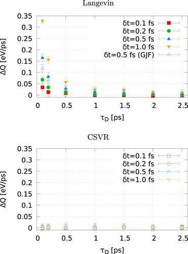The different of these two heats, $\mathrm{\Delta }Q=(Q_{hot}-Q_{cold})$ as a function of the damping time and the timestep used to integrate the equations of motion can be used a criterion to assess the stability of the non-equilibrium trajectory. $\mathrm{\Delta }Q$ increases (see Figure 4 and red and blue curves in Figure 3 top-left) with long timesteps and short damping times. Short time steps lead to a considerable improvement of the stability of the trajectory; see results for 0.1 fs in Figure 4. However, reducing the timestep to this value leads to a loss of computational efficiency, which is not desirable. Again, the CSVR thermostat shows much better stability across the whole range of timesteps and damping times investigated, offering a better alternative to performing the non-equilibrium simulations. Note that with the langevin/gjf algorithm, the heat rate of the hot and cold thermostats is also different at very short damping times (see Figure 4), although the difference is smaller than that of the original Langevin thermostat. This is connected to the fact that the damping time is much shorter than the characteristic relaxation time of the heat flux (see Figure 1).

Figure 4. (Colour online) Heat rate difference between the hot and cold thermostats for Langevin (left) and canonical velocity rescaling (right), as a function of the damping time, ${\tau }_D$, for different integration timesteps $\delta t$.

The discussion above shows that the energy conservation using the Langevin thermostat is heavily affected by the magnitude of the damping time. Longer damping times or shorter time steps are preferred to conserve energy and define the heat flux properly. 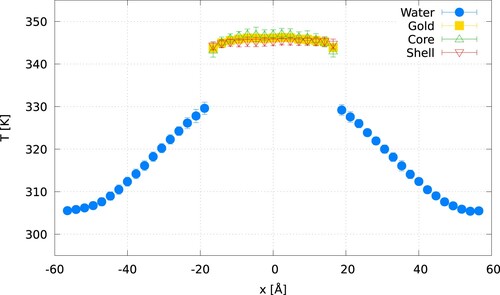In addition to the heat flux, $J_q$, the calculation of the thermal conductance, G, using NEMD requires the computation of the temperature ‘jump’, $\mathrm{\Delta }T$, across the interface, (7) $G=\frac{J_q}{\mathrm{\Delta }T}.$(7) Figure 5 shows representative temperature profiles for gold-water systems using the Langevin and CSVR thermostats. All the temperature profiles feature a well-defined temperature ‘jump’. We used the temperature difference at the gold-water interface to estimate $\mathrm{\Delta }T$ by fitting the temperature profiles to linear functions (shown as dashed lines in Figure 5) in a region spanning three atomic layers in gold and an equivalent distance for the fluid phase. The temperature ‘jump’ was estimated by evaluating the linear fits at the position of the interface, $x_i=\pm a{N}_l\sqrt{3}/6$, where $x_i$ is the coordinate of the gold surfaces, a is the lattice constant and $N_l$ is the number of atomic layers in the gold slab (indicated by the lines with arrows in Figure 5). The intersection of the regression lines with the interface plane defines the temperatures, $T_W$ and $T_{Au}$, and the interfacial temperature ‘jump’, $\mathrm{\Delta }T=T_{Au}-T_W$. The temperature of the oxygen and hydrogen atoms was calculated by assuming equipartition of the kinetic energy between the translational and rotational degrees of freedom of the rigid water molecule.

Figure 5. (Colour online) Temperature profiles obtained using the Langevin or CSVR thermostats with a damping time ${\tau }_D=0.1\mathrm{ps}$ (top) or ${\tau }_D=2.5$ (bottom). Both thermostats are applied to all the particles (core and shell) in the gold slab. For all the panels, the empty symbols represent the temperatures of the core or shell atoms, highlighting their temperature differences.‘Gold’ refers to the average temperature obtained using the temperatures of the core and shell particles. The arrows signal the interfacial region used to calculate the temperature jump.

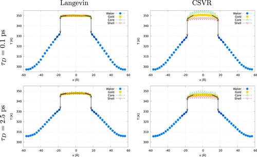
In all cases, the temperature profiles obtained with the Langevin thermostat show that the two particles in the gold slab, core and shell, are at the same temperature. For both the Langevin and CSVR thermostats, the shorter damping times lead to an average slab temperature closer to the target temperature of 350 K, while for longer damping, the temperature is below or above the target one for hot or cold thermostats, respectively. The differences between the calculated temperatures and the set ones can be explained in terms of the decreasing strength of the coupling with the heat bath at larger damping times. This effect has been observed in NEMD simulations of thermal transport in silicon [22].

The temperature profiles obtained with CSVR reveal some problems with this thermostatting approach. The temperatures of the gold-core and shell particles are different, with an average temperature difference of 5.9 K (${\tau }_D=0.1\mathrm{ps}$) and 3.6 K (${\tau }_D=2.5\mathrm{ps}$). While the CSVR thermostatting approach leads to the correct average target temperature, it breaks equipartition between the core and shell particles, as indicated by their different stationary temperatures This issue is problematic since the calculation of the thermal conductance in NEMD requires a precise estimate of the temperature ‘jump’. We explain below a procedure to solve this problem in the CSVR thermostat and assess its impact on the temperature ‘anisotropy’ on the computed thermal conductances.

Figure 6 shows results for the thermal conductances obtained with the Langevin and CSVR thermostats as a function of the simulation timestep and the damping time. For the calculations, we used two approaches: the average heat flux obtained from the energy exchanged in both thermostats or the heat flux obtained with the energy exchanged in the cold thermostat (which acts on water), only. The thermal conductances obtained with the Langevin thermostat and using the average heat flux show a strong dependence with both the damping time and the timestep. Short damping times, 0.1 ps, result in high thermal conductances, 784 MW/(m${}^2$ K), which decrease down to 647 MW/(m${}^2$ K) for the same damping time and a short time step (0.1 fs). These values reflect the impact of lack of energy conservation reported in Figure 3. There is also a clear dependence of the thermal conductance with the damping time for the same simulation timestep (see, e.g. symbols for $\delta t=0.1\mathrm{fs}$ and ${\tau }_D=0.1-2.5\mathrm{ps}$ in Figure 4(a)). Long relaxation times result in even lower thermal conductances, 524 MW/(m${}^2$ K) for ${\tau }_D=2.5\mathrm{ps}$ and $\delta t=0.1\mathrm{fs}$. Damping times longer than 1.5 ps do not influence the thermal conductance significantly. The results obtained with the CSVR thermostat show no significant dependence on ${\tau }_D$ and a small dependence on $\delta t$, with long time steps giving slightly higher thermal conductances. The timestep length is important when considering vibrational degrees of freedom, such as those included in the polarisable Drude model employed here. For the force constant and masses reported above, we get the ${\nu }_{Drude}=1.6\times {10}^{14}{\mathrm{s}}^{-1}$. To define the oscillatory motion accurately, a timestep of $\delta t\sim {\nu }_{Drude}^{-1}/10$ is desirable, giving a timestep of about 0.6 fs. Figure 6 shows that thermal conductances obtained with a time step of this order or lower are consistent with each other. At the same time, longer timesteps (1 fs) result in significant deviations of the thermal conductances obtained with either the Langevin or the CSVR thermostats. The heat fluxes used to estimate the thermal conductance also introduce some differences for the original Langevin and the Langevin/GJF thermostats and short damping times. The heat flux obtained from the average of the energy exchanged at both thermostats results in very high thermal conductance. The thermal conductance obtained with the energy exchanged in the cold thermostat is, as expected, lower but still far from the values obtained with the optimum conditions (longer damping and shorter timestep). The differences between these two approaches to compute the heat flux simply reflect the lack of energy conservation reported in Figure 3.

Figure 6. (Colour online) Thermal conductance for Langevin (top) and canonical velocity rescale (bottom) thermostats, as a function of the thermostat damping time. The thermal conductance was computed using the average of the energy exchanged in the hot and cold thermostats (filled points), or just the cold thermostat (empty points).

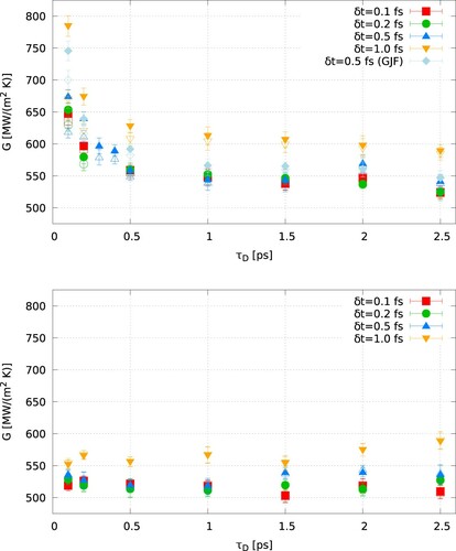
Table 2. Thermal conductances obtained in this work using different thermostats and damping constants.

		G [MW/(m${}^2$ K)]
$\delta t$ [fs]	${\tau }_D$ [ps]	Langevin	CSVR
0.5	0.1	$674\pm 10$ ($619\pm 10$)	$536\pm 8$ ($535\pm 8$)
0.5	2.5	$542\pm 10$ ($539\pm 11$)	$536\pm 14$ ($538\pm 14$)

Note: The results in parenthesis were obtained using the heat flux obtained from the energy exchanged at the cold thermostat only. The other results were obtained using the average of the heat fluxes of the cold and hot thermostat.

The main conclusion from the results presented above is that the Langevin thermostat leads to significant deviations in the computation of the thermal conductance. Generally, short time steps and long damping times lead to convergence of the simulated thermal conductances. The thermal conductance obtained with the CSVR thermostat features a small dependence with the timestep ($\delta t\ge 0.5\mathrm{fs}$) while it is independent of the damping time in the interval ${\tau }_D=0.1-2.5\mathrm{ps}$. The thermal conductance obtained with these two thermostats at the ‘optimum’ conditions are similar, 542 and 536 MW/(m${}^2$ K) (see Table 2). Overall, our results indicate that the type of thermostat employed in NEMD needs to be chosen with care when computing thermal conductances.

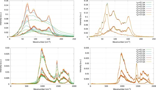
One question arising from our results is why the thermal conductances obtained with the Langevin thermostat depend so strongly on the damping time. This question can be addressed by computing the vibrational density of states (VDOS) and the heat flux correlation functions. We show in Figure 7 the VDOS of the interfacial gold atoms (the atoms in the surface layers of the gold slab) and water molecules in the interfacial region (highlighted in Figure 2, see green shadowed area). The VDOS of the water molecules, obtained with the optimum conditions for the Langevin thermostat, shows significant overlap with both the VDOS of the core and shell particles (see Figure 7). Figure 8 shows the impact of the Langevin and CSVR thermostats on the VDOS of gold for different damping times. Short damping times and the Langevin thermostat lead to a strong perturbation of the VDOS of the core particles. The distribution becomes wider, and the intensity of the peaks decreases (see the top-left panel in Figure 8). This result is in line with recent reports using this thermostat for purely atomistic solids [22]. The damping constant does not influence the density of states of the interfacial water molecules. The VDOS obtained with the CSVR thermostat is insensitive to the damping constant. This result is consistent with the lack of significant dependence observed in the thermal conductances that we reported above for this thermostat (see Figure 6). The substantial changes introduced by the Langevin thermostat in the VDOS of the core particles are correlated with the modification of the heat flux relaxation times. The relaxation time is given by the autocorrelation function (see Figure 1). For the model of polarisable gold employed here, the relaxation time (at NVE conditions) is $\sim$0.04 ps. However, when the heat flux autocorrelation function is computed only for the core particles, we obtain a relaxation time of $\sim$1.4 ps, much longer. This long relaxation time explains the need to increase the damping time to longer values, such as ∼2.5 ps, which lead to better energy conservation (see Figure 3). Also, it explains why the VDOS shows good convergence with the CSVR results (see Figure 8(a)) when we use longer damping times.

Figure 7. (Colour online) Vibrational density of states for the core (green) and shell (red) particles, and water (blue), using the Langevin thermostat with ${\tau }_D=2.5\mathrm{ps}$ for the gold slab. Individual components are shown with dashed (component parallel to heat flux) and dotted (component perpendicular to heat flux) lines. The total VDOS is calculated as the sum the three components, x, y and z. The VDOS of water shows significant overlap with both the core and shell particles.

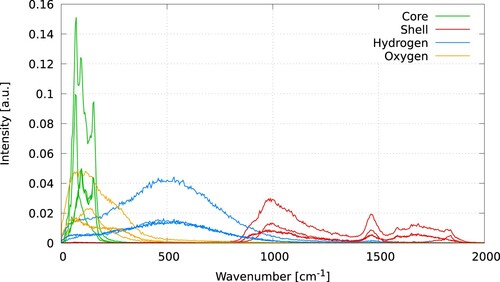
Figure 8. (Colour online) VDOS of the interfacial region, for the core (top) and shell (bottom) particles. The left (right) panels correspond to Langevin (CSVR) thermostats with different damping parameters.⁣⁣⁣⁣⁣⁣⁣

We have shown above that the width of the VDOS obtained with the Langevin thermostat increase significantly at short damping times. We analyse here the impact of these changes in VDOS on the overlap of the VDOS of gold and water, by calculating, (8) $S_{\alpha \beta }=\frac{{\int }_0^{\mathrm{\infty }}{D}_{\alpha }(\omega )D_{\beta }(\omega )\mathrm{d}\omega }{{\int }_0^{\mathrm{\infty }}{D}_{\alpha }(\omega )\mathrm{d}\omega {\int }_0^{\mathrm{\infty }}{D}_{\beta }(\omega )\mathrm{d}\omega }$(8) where $D_{\alpha }$ and $D_{\beta }$ 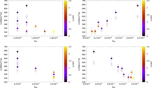are the density of states of the different atomic species. S increases with the overlap, and it was used in reference [38,39] to explain the changes in the thermal conductance of solid-solid interfaces. We show in Figure 9 the correlation plots between the thermal conductance and the overlapping, S, between different pairs of atoms and using the Langevin thermostat. The thermal conductance shows a correlation with the overlap between the hydrogen atoms and the core particles. The overlap becomes stronger at short damping times, where we observe higher conductances. This result supports our view that a large increase in G, as observed with the Langevin thermostat at short damping times, arises from the broadening of the VDOS of gold and the enhanced overlap between the vibrational modes of the core particles of gold and the hydrogen. While the oxygen power spectrum is associated to the intermolecular vibrations, the faster hydrogen modes arise from the librations of the water molecules [40,41], which we identify as the key contributor to the interfacial thermal conductance in the system studied here. As the damping time increases the VDOS approaches the equilibrium spectrum, and the thermal conductance obtained with the Langevin thermostat converges to values consistent with the CSVR thermostat. The important role of the core-hydrogen correlations can be assessed by calculating the overlap between other atomic pairs. The increased overlap of the shell-hydrogen, shell-oxygen and core-oxygen functions is not correlated with the enhancement of the thermal conductance observed in the simulations (see Figure 8).

Figure 9. (Colour online) Interfacial thermal conductance as a function of the VDOS overlap, S, between different atomic species. The calculations correspond to the Langevin thermostat applied to the gold atoms (core and shell). The heat flux has been calculated using the energy exchanged in both thermostats (filled symbols), or just the water thermostat (open symbols).

We conclude that the CSVR thermostat offers a better approach than the Langevin one since the former has little impact on the VDOS, and G features a weak dependence with either the timestep or the damping constant. However, this thermostat results in a breakdown of equipartition for the solid considered here, which includes intramolecular degrees of freedom (core-shell particles with large mass differences). To circumvent this problem, we implemented a ‘dual’ CSVR thermostat to ensure the temperatures of core and shell particles are consistently defined. The thermostats are applied separately to the core and shell particles in gold. Figure 10 shows the temperature profiles for the dual CSVR thermostat. A direct comparison with Figure 5 evidences that the use of a dual thermostat applied on individual degrees of freedom reduces the temperature difference between the core and shell particles, which have the same temperature within the statistical uncertainty of our computations.

Figure 10. (Colour online) Temperature profile using the dual CSVR thermostat with ${\tau }_D=2.5\mathrm{ps}$ and $\delta t=0.5\mathrm{fs}$.

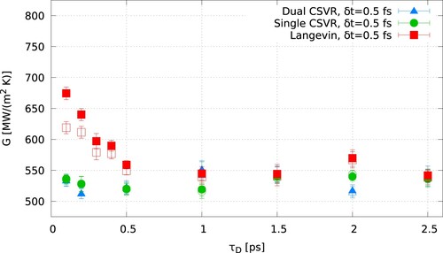
In Figure 11, we compare the interfacial thermal conductance for the 3 different thermostatting approaches investigated here, and $\delta t=0.5\mathrm{fs}$. Both CSVR thermostats (single or dual) show very similar results, and the thermal conductance does not feature a significant dependence with damping time. The thermal conductance obtained with the Langevin thermostat converges to the CSVR values at long damping times (${\tau }_D>1.5\mathrm{ps}$).

Figure 11. (Colour online) Comparison of the interfacial thermal conductance obtained with the 3 different thermostatting configurations. All the results were obtained with $\delta t=0.5\mathrm{fs}$.

4. Conclusions

The Langevin thermostat acts ‘locally’ on each particle, and therefore it has a considerable impact on the vibrational density of states (VDOS) of polarisable solids modelled with the Drude oscillators. Short damping times lead to a broadening of the VDOS and an artificial increase (up to 40%) of the thermal conductance and violation of energy conservation. The enhancement of the thermal conductance correlates with the increasing overlap of the interfacial VDOS of gold and water. Converging ITCs can be obtained using thermostatting damping times longer than the characteristic heat flux relaxation time of the solid of interest, $>2$ ps, for the gold model employed here.

Global thermostats such as the canonical velocity rescaling predict ITCs nearly independent of the damping constant. However, they introduce a break of equipartition in the Drude particles, manifested in different temperatures of the core and shell sites. This effect is likely connected to the large mass difference of the shell/core sites typically used in Drude polarisable models. We have proposed a solution to this problem that relies on using a dual thermostat for both core and shell sites.

Overall our work highlights the importance of the thermostatting approach used in NEMD simulations of the ITC. We expect these effects will be relevant in many systems. We have studied the impact of thermostatting on a polarisable solid, but the Drude approach is widely employed in molecules, too; hence thermostatting should be exercised with care in that case.

Disclosure statement

No potential conflict of interest was reported by the author(s).

Additional information

Funding

Financial support from the Leverhulme Trust (grant RPG-2018-384), and computational resources from the Imperial College High Performance Computing Service are gratefully acknowledged.

References

- Kapitza PL. Heat transfer and superfluidity of helium II. Phys Rev. 1941 Aug;60:354–355. Available from: https://link.aps.org/doi/https://doi.org/10.1103/PhysRev.60.354.
- Swartz ET, Pohl RO. Thermal boundary resistance. Rev Mod Phys. 1989 Jul;61:605–668. Available from: https://link.aps.org/doi/https://doi.org/10.1103/RevModPhys.61.605.
- Cahill DG, Braun PV, Chen G, et al. Nanoscale thermal transport. II. 2003–2012. Appl Phys Rev. 2014;1(1):Article ID 011305. Available from: https://doi.org/https://doi.org/10.1063/1.4832615.
- Ge Z, Cahill DG, Braun PV. Thermal conductance of hydrophilic and hydrophobic interfaces. Phys Rev Lett. 2006 May;96:Article ID 186101. Available from: https://link.aps.org/doi/https://doi.org/10.1103/PhysRevLett.96.186101.
- Bresme F, Lervik A, Armstrong J. Chapter 6 non-equilibrium molecular dynamics. In: Experimental thermodynamics volume X: non-equilibrium thermodynamics with applications. The Royal Society of Chemistry; 2016. p. 105–133. Available from: https://doi.org/http://dx.doi.org/10.1039/9781782622543-00105.
- Patel HA, Garde S, Keblinski P. Thermal resistance of nanoscopic liquid-liquid interfaces: dependence on chemistry and molecular architecture. Nano Lett. 2005 Nov;5(11):2225–2231. Available from: https://doi.org/https://doi.org/10.1021/nl051526q.
- Alexeev D, Chen J, Walther JH, et al. Kapitza resistance between few-layer graphene and water: liquid layering effects. Nano Lett. 2015 Sep;15(9):5744–5749. Available from: https://doi.org/https://doi.org/10.1021/acs.nanolett.5b03024.
- Bhattarai H, Newman KE, Gezelter JD. The role of polarizability in the interfacial thermal conductance at the gold-water interface. J Chem Phys. 2020;153(20):Article ID 204703. Available from: https://doi.org/https://doi.org/10.1063/5.0027847.
- Shenogina N, Godawat R, Keblinski P, et al. How wetting and adhesion affect thermal conductance of a range of hydrophobic to hydrophilic aqueous interfaces. Phys Rev Lett. 2009 Apr;102:Article ID 156101. Available from: https://link.aps.org/doi/https://doi.org/10.1103/PhysRevLett.102.156101.
- Lervik A, Bresme F, Kjelstrup S. Heat transfer in soft nanoscale interfaces: the influence of interface curvature. Soft Matter. 2009;5:2407–2414. Available from: https://doi.org/http://dx.doi.org/10.1039/B817666C.
- Tascini AS, Armstrong J, Chiavazzo E, et al. Thermal transport across nanoparticle-fluid interfaces: the interplay of interfacial curvature and nanoparticle-fluid interactions. Phys Chem Chem Phys. 2017;19:3244–3253. Available from: https://doi.org/http://dx.doi.org/10.1039/C6CP06403E.
- Hu M, Poulikakos D, Grigoropoulos CP, et al. Recrystallization of picosecond laser-melted ZnO nanoparticles in a liquid: a molecular dynamics study. J Chem Phys. 2010;132(16):Article ID 164504. Available from: https://doi.org/https://doi.org/10.1063/1.3407438.
- Neidhart SM, Gezelter JD. Thermal transport is influenced by nanoparticle morphology: a molecular dynamics study. J Phys Chem C. 2018;122(2):1430–1436. Available from: https://doi.org/https://doi.org/10.1021/acs.jpcc.7b12362.
- Xue L, Keblinski P, Phillpot SR, et al. Two regimes of thermal resistance at a liquid-solid interface. J Chem Phys. 2003;118(1):337–339. Available from: https://doi.org/https://doi.org/10.1063/1.1525806.
- Muscatello J, Chacón E, Tarazona P, et al. Deconstructing temperature gradients across fluid interfaces: the structural origin of the thermal resistance of liquid-vapor interfaces. Phys Rev Lett. 2017 Jul;119:Article ID 045901. Available from: https://link.aps.org/doi/https://doi.org/10.1103/PhysRevLett.119.045901.
- Volz SG, Chen G. Molecular-dynamics simulation of thermal conductivity of silicon crystals. Phys Rev B. 2000 Jan;61:2651–2656. Available from: https://link.aps.org/doi/https://doi.org/10.1103/PhysRevB.61.2651.
- Schelling PK, Phillpot SR, Keblinski P. Comparison of atomic-level simulation methods for computing thermal conductivity. Phys Rev B. 2002 Apr;65:Article ID 144306. Available from: https://link.aps.org/doi/https://doi.org/10.1103/PhysRevB.65.144306.
- Sellan DP, Landry ES, Turney JE, et al. Size effects in molecular dynamics thermal conductivity predictions. Phys Rev B. 2010 Jun;81:Article ID 214305. Available from: https://link.aps.org/doi/https://doi.org/10.1103/PhysRevB.81.214305.
- Iriarte-Carretero I, Gonzalez MA, Bresme F. Thermal conductivity of ice polymorphs: a computational study. Phys Chem Chem Phys. 2018;20:11028–11036. Available from: https://doi.org/http://dx.doi.org/10.1039/C8CP01272E.
- Li Z, Xiong S, Sievers C, et al. Influence of thermostatting on nonequilibrium molecular dynamics simulations of heat conduction in solids. J Chem Phys. 2019;151(23):Article ID 234105. Available from: https://doi.org/https://doi.org/10.1063/1.5132543.
- Daub CD, Åstrand PO, Bresme F. Thermo-molecular orientation effects in fluids of dipolar dumbbells. Phys Chem Chem Phys. 2014;16:22097–22106. Available from: https://doi.org/http://dx.doi.org/10.1039/C4CP03511A.
- Dunn J, Antillon E, Maassen J, et al. Role of energy distribution in contacts on thermal transport in SI: a molecular dynamics study. J Appl Phys. 2016;120(22):Article ID 225112. Available from: https://doi.org/https://doi.org/10.1063/1.4971254.
- Ghatage D, Tomar G, Shukla RK. Thermostat-induced spurious interfacial resistance in non-equilibrium molecular dynamics simulations of solid–liquid and solid–solid systems. J Chem Phys. 2020;153(16):Article ID 164110. Available from: https://doi.org/https://doi.org/10.1063/5.0019665.
- Geada IL, Ramezani-Dakhel H, Jamil T, et al. Insight into induced charges at metal surfaces and biointerfaces using a polarizable Lennard-Jones potential. Nat Commun. 2018;9(1):1–14. Available from: https://doi.org/http://dx.doi.org/10.1038/s41467-018-03137-8.
- Bussi G, Donadio D, Parrinello M. Canonical sampling through velocity rescaling. J Chem Phys. 2007;126(1). https://doi.org/https://doi.org/10.1063/1.2408420
- Dünweg B, Paul W. Brownian dynamics simulations without gaussian random numbers. Int J Mod Phys C. 1991;2(3):817–827. Available from: https://doi.org/https://doi.org/10.1142/S0129183191001037.
- Berendsen HJC, Grigera JR, Straatsma TP. The missing term in effective pair potentials. J Phys Chem. 1987;91(24):6269–6271. Available from: https://doi.org/https://doi.org/10.1021/j100308a038.
- Ryckaert JP, Ciccotti G, Berendsen HJ. Numerical integration of the cartesian equations of motion of a system with constraints: molecular dynamics of n-alkanes. J Comput Phys. 1977;23(3):327–341. Available from: https://www.sciencedirect.com/science/article/pii/0021999177900985.
- Schneider T, Stoll E. Molecular-dynamics study of a three-dimensional one-component model for distortive phase transitions. Phys Rev B. 1978 Feb;17:1302–1322. Available from: https://link.aps.org/doi/https://doi.org/10.1103/PhysRevB.17.1302.
- Brünger A, Brooks CL, Karplus M. Stochastic boundary conditions for molecular dynamics simulations of ST2 water. Chem Phys Lett. 1984;105(5):495–500. Available from: https://www.sciencedirect.com/science/article/pii/0009261484800986.
- Grønbech-Jensen N, Farago O. A simple and effective Verlet-type algorithm for simulating Langevin dynamics. Mol Phys. 2013;111(8):983–991. Available from: https://doi.org/https://doi.org/10.1080/00268976.2012.760055.
- Plimpton S. Fast parallel algorithms for short-range molecular dynamics. J Comput Phys. 1995;117(1):1–19. Available from: https://www.sciencedirect.com/science/article/pii/S002199918571039X.
- Woodcock L. Isothermal molecular dynamics calculations for liquid salts. Chem Phys Lett. 1971;10(3):257–261. Available from: https://www.sciencedirect.com/science/article/pii/0009261471802816.
- Lemak AS, Balabaev NK. On the Berendsen thermostat. Mol Simul. 1994;13(3):177–187. Available from: https://doi.org/https://doi.org/10.1080/08927029408021981.
- Harvey SC, Tan RKZ, Cheatham III TE. The flying ice cube: velocity rescaling in molecular dynamics leads to violation of energy equipartition. J Comput Chem. 1998;19(7):726–740. Available from: https://onlinelibrary.wiley.com/doi/abs/https://doi.org/10.1002/(SICI)1096-987X(199805)19:7%3C726::AID-JCC4%3E3.0.CO%3B2-S.
- Braun E, Moosavi SM, Smit B. Anomalous effects of velocity rescaling algorithms: the flying ice cube effect revisited. J Chem Theory Comput. 2018;14(10):5262–5272. PMID: 30075070; Available from: https://doi.org/https://doi.org/10.1021/acs.jctc.8b00446.
- Irving JH, Kirkwood JG. The statistical mechanical theory of transport processes. IV. the equations of hydrodynamics. J Chem Phys. 1950;18(6):817–829. Available from: https://doi.org/https://doi.org/10.1063/1.1747782.
- Li B, Lan J, Wang L. Interface thermal resistance between dissimilar anharmonic lattices. Phys Rev Lett. 2005 Sep;95:Article ID 104302. Available from: https://link.aps.org/doi/https://doi.org/10.1103/PhysRevLett.95.104302.
- Yang N, Zhang G, Li B. Carbon nanocone: a promising thermal rectifier. Appl Phys Lett. 2008;93(24):Article ID 243111. Available from: https://doi.org/https://doi.org/10.1063/1.3049603.
- Impey R, Madden P, McDonald I. Spectroscopic and transport properties of water. Mol Phys. 1982;46(3):513–539. Available from: https://doi.org/https://doi.org/10.1080/00268978200101361.
- Fois E, Gamba A, Redaelli C. Hydrophobic effects: a computer simulation study of the temperature influence in dilute O2 aqueous solutions. J Chem Phys. 1999;110(2):1025–1035. Available from: https://doi.org/https://doi.org/10.1063/1.478147.