Improved estimation of ultra-deep water pipe collapse pressures by using extreme value theory

Abstract

We examine safety margins between measured pipe collapse pressures and maximum external hydrostatic pressure exerted on pipeline on the seabed. We analyze collapse pressures measured on specimen rings cut from pipes, which are valid proxies for testing full length pipes. Our novel application of statistical models motivated by Extreme Value Theory provides a firmer basis for extrapolating collapse pressures than current practice which assumes a Gaussian distribution, and which gives over-conservative safety margins compared with our method. Our more accurate assessment of collapse pressures could give large cost savings in the manufacture of thick-walled pipe for ultra-deep water pipelines.

Keywords:

• Bayesian methods
• non-normal data
• probability distributions
• process improvement
• product reliability
• statistical modeling

Introduction

Over the past 20 years there has been considerable development in the design, manufacture, installation and operation of thick-walled pipelines in ultra-deep water. Design guidance in DNVGL OS F101 (2013) determines safety from pressure collapse failure during pipeline installation theoretically using empirical formulas. There are huge financial implications of loss of a very long pipeline during installation in ultra-deep water, so pipeline design is commonly validated further using pipe joint collapse tests. Pressure testing full-scale pipe joints is an expensive undertaking that requires a suitable pressure chamber. Walker, Chee, and Roberts (2017) describe an alternative approach to obtain collapse pressure data first introduced by Slater et al. (2011). In their approach, costly full-scale pipe tests are replaced by tests on ring specimens cut and machined from manufactured pipe joints. This innovation allows data on pipe collapse pressures to be collected in sufficient quantity to make statistical modeling of collapse pressure feasible. The current article presents a novel application of statistical models motivated by Extreme Value Theory (EVT) (Coles 2001) to data from ring tests.

Design criteria for installation require the probability of collapse to be around 1e − 07. The collapse event is sufficiently rare as to be effectively unobservable from any data sample of a practical and economically feasible size. Statistical models motivated by EVT have been developed expressly for the estimation of occurrence probabilities of extremely rare events. Many applications in engineering, environmental science, finance and others require estimation of the risk of rare events (such events include flooding, financial crashes, extreme loadings on structures caused by large weather events, etc.). These catastrophic events often lie well beyond levels observed in available data. Statisticians are naturally wary of extrapolating their fitted models beyond levels at which data can be used to validate model fit. Many practical applications therefore rely on statistical models motivated by EVT which provides additional theoretical justification for model extrapolation. EVT has been established for many years and offers a practical solution to the challenge of estimating the risk of rare events: see Finkenstadt and Rootzèn (2003), Coles (2001), and references therein. Statistical models motivated by EVT are widely used in coastal and offshore engineering applications where methods specifically suited to this setting have been developed by Haigh, Nicholls, and Wells (2010), Tawn (1992), and Dhanak and Xiros (2016). There is some history of these models being used in manufacturing engineering but the methods are still considered somewhat esoteric, Anderson et al. (2003) and Fougères, Holm, and Rootzèn (2006). Here we hope to illustrate the value of the proposed methods in this setting.

Current practice (Selker, Ramos, and Liu 2015) fits the ring test results with a Gaussian distribution of collapse pressures. Although that article is only meant to present typical statistical distribution for the central mass of the test results, one could quickly extrapolate this distribution to derive collapse pressures corresponding to tiny probabilities of collapse. We show that this approach overestimates the probability of collapse at external pressures, leading to grossly conservative safety margins. This raises a number of questions for an industry which is required to balance the safety of such installations with the reasonable expense of manufacture and installation. Our findings suggest that dramatic cost savings may be possible, whilst retaining an acceptable level of safety assurance.

The article is structured as follows: we introduce the proposed statistical modeling approach. We then describe detailed analysis of the data set, including the use of model diagnostics motivated by EVT. We go on to estimate the extrapolated collapse pressures of interest and assess sensitivity of these results to a range of features of our approach. We compare our results and conclusions with those derived from existing methods. Finally, we address some practical considerations for our proposed method in practice and conclude with a discussion of the potential wider impact of our approach.

Description of proposed statistical methodology

We propose the use of a threshold-based statistical model to describe the tail of collapse pressure data from ring tests. This model was introduced by Davison and Smith (1990), and provides an extremely flexible family of parametric models which can be used to extrapolate tail behavior beyond levels observed in data. The form of the model is derived from EVT (Leadbetter, Lindgren, and Rootzén 2012). This theory supplies an asymptotic justification for the form of model appropriate to describing the tails of probability distributions. The theory also motivates a collection of model diagnostics which are necessary to support our confidence in the model assumptions which underpin the extrapolation process.

The generalized Pareto distribution

We use the generalized Pareto distribution (GPD) ($\sigma ,\xi$) (Davison and Smith 1990), fitted to data beyond a suitably chosen threshold. In the literature, the GPD is usually expressed in its upper tail form, describing excesses over thresholds. We follow this format here; lower tail formulation is entirely equivalent. This statistical model arises from an asymptotic argument describing the behavior of random variables given that they exceed a threshold. EVT describes the full range of possible limiting behavior as the threshold increases to the upper limit of the underlying distribution. We assume variable X follows a GPD above a threshold u so that $X|X>u\sim$ GPD (${\sigma }_u,\xi$) with distribution function $$\text{Pr}(X<x|X>u)=1-{\left\{1+\xi \left(\frac{x-u}{{\sigma }_u}\right)\right\}}^{-1/\xi }\text{for}x>u,$$ where u is the threshold for fitting and ${\sigma }_u>0$ and −∞<ξ<∞ IR are scale and shape parameter, respectively. The shape parameter determines the manner in which the tail approaches its upper bound (this bound may be infinite). The distribution has a finite upper end point (short tailed) if the shape parameter is negative ($u<x\le u-{\sigma }_u/\xi$ if $\xi <0$) and an infinite tail otherwise ($u<x<\infty$ if $\xi \ge 0$). When ξ = 0, the GPD corresponds exactly to the Exponential distribution.

For x > u, the unconditional distribution of X is given by $$\text{Pr}(X<x)=1-\text{Pr}(X>x)=1-\text{Pr}(X>x|X>u\left)\text{Pr}\right(X>u)\text{for}x>u.$$

For application to data, the conditional probability $\text{Pr}(X>x|X>u)$ is estimated by using the fitted GPD and the probability of threshold excess $\text{Pr}(X>u)$ is estimated empirically by the proportion of datapoints exceeding the threshold u.

EVT tells us that as the threshold u tends to the distributional upper endpoint, the limiting distribution of the excesses must fall in the generalized Pareto family of distributions (given certain conditions concerning non-degeneracy of the limit distribution and smoothness of the distribution of the original variable). So whatever the original distribution of collapse pressure measurements, provided we choose an appropriate threshold, the conditional distribution of values beyond that threshold, given that they lie beyond the threshold, should be well approximated by a GPD. In practice, this asymptotic theory is applied at finite thresholds and so it is important to check necessary conditions for the suitability of the chosen threshold. These conditions motivate a range of diagnostic tools which we describe next.

Threshold selection

A crucial step in the fitting of the GPD is the selection of an appropriate threshold. EVT tells us that if a suitable threshold can be chosen, then the GPD is the appropriate model for values beyond this threshold, but it does not tell us what the threshold should be. We use two threshold diagnostics, which exploit the theoretical properties of the GPD to aid selection of a suitable threshold (Coles 2001). We describe these diagnostics now.

Mean residual life (MRL) plot

This diagnostic requires $\xi <1$ for expectations to be defined. It uses the linearity of the conditional mean excess function, defined as follows: for X as above, the mean excess of X over u is $$E(X-u|X>u)=\frac{{\sigma }_u}{1-\xi }.$$

The mean excess of X over v > u is linear in v with gradient $\xi /(1-\xi )$ $$E(X-v|X>v)=\frac{{\sigma }_u+v\xi }{1-\xi }$$

We plot the estimated mean excess above threshold against threshold for a range of threshold values. The plot will be approximately linear (up to estimation uncertainty) beyond an appropriately chosen threshold. The sign of the gradient in the linear part of the plot corresponds to the sign of the GPD shape parameter and hence indicates the tail shape. Negative gradient shows a short-tailed distribution, zero gradient shows an exponential type tail and a positive gradient suggests a heavy tailed distribution.

Threshold stability plot

We use a re-parametrization of the GPD, to $({\sigma }_m,\xi )$, where ${\sigma }_m={\sigma }_u-\xi u$ is a threshold-invariant version of the scale parameter σ_u, as its value does not vary with u. We plot estimates of $({\sigma }_m,\xi )$ against threshold over a range threshold values. The parameter estimates will be approximately constant above a suitably chosen threshold (up to estimation uncertainty).

Parameter estimation

The performance of parameter estimation procedures depends on the underlying parameter values themselves, specifically the shape parameter ξ. For all values of ξ greater than −1, maximum likelihood estimation of model parameters is consistent (as the sample size increases, the sampling distribution of the estimator increasingly concentrates around the true parameter value). However for $-1<\xi <-0.5$ (encountered in this application) the limit distributions of maximum likelihood estimators are non-normal (Smith 1987). This means that standard methods for deriving uncertainty summaries, including confidence interval calculation using the normal approximation, are not appropriate. We use Bayesian Markov Chain Monte Carlo (MCMC) methods to estimate model parameters and quantiles, with credible intervals to describe estimation uncertainty, Gilks, Richardson, and Spiegelhalter (1995). In practice, we work with ${\varphi }_u=\hspace{0.17em}\text{log}\hspace{0.17em}{\sigma }_u$, to aid numerical stability.

Application to pipe collapse data

The Appendix contains a copy of the original data and code to reproduce the article’s central analysis. We use R (R Core Team 2016), and the extreme values package texmex (Southworth, Heffernan, and Metcalfe 2016) for our analysis.

Collapse pressure measurements

In the example analyzed in this article, 32 in. diameter pipeline is intended for operation at a maximum water depth of 2,200 m. DNVGL formulas which provide guidance for pipe design require a design wall thickness of 36.5 mm for a maximum water depth of 2,200 m. Ultimately, a wall thickness of 39 mm was preferred for the project, which DNVGL calculates as providing a collapse pressure equivalent to 2,475 m water depth, giving an additional level of safety. DNVGL regulations require checks on two limit states: system collapse (pure collapse) and local buckling (combined with bending and axial force). The discussion presented in this work relates to collapse resistance.

Walker, Chee, and Roberts (2017) demonstrated that results from ring tests can be regarded as a viable proxy for pipe full-body collapse testing. We use collapse pressure data from 158 ring tests. These data represent collapse pressures measured on rings cut from unique pipes, from different manufacturing runs. The pipes shared identical specifications for materials, geometric properties and inspection requirements. Rings were prepared using the same procedure and tested using the same equipment. As such it is appropriate to assume that these collapse pressures represent statistically independent and identically distributed measurements which capture both pipe to pipe and long-term manufacturing variability in collapse pressure. The ring test procedure ensures that test results are consistent from one ring to another. By slowly increasing the pressure applied to the pressure chamber in the test, the loading on the ring replicates the conditions that would be applied to the pipe as it is lowered onto the seabed. Collapse pressures are measured in MPa and recorded to 1 decimal place resulting in some ties in the data. We therefore analyze the data as interval censored throughout.

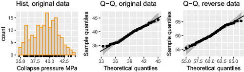
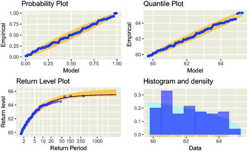
Figure 1 shows a histogram of the data which have an approximately bell or triangular-shaped distribution, with a single mode lying roughly centrally. The distinct data values are shown on the horizontal axis.

Figure 1. Histogram of original collapse pressure data and Q–Q plots for Normal model fitted to both original and reverse collapse pressures (MPa).

GPD fit to collapse pressure data

Interest is in the lower tail of the collapse pressure distribution, as this describes the potential behavior of the weakest pipes. EVT motivated statistical methods and associated software are generally set up for upper tail modeling, so we transform the data so that we can work with the upper tail and avoid having to re-express methods in their lower tail equivalents or re-write software. Model fitting following transformation is entirely equivalent. The original collapse pressure observations are transformed by negation and then adding 100 to the negated pressures so that the resulting values are positive. We refer to these transformed values as reverse collapse pressures. The transformation is linear, so results are correct when extrapolated values from the reverse collapse pressure scale are transformed back to the original scale by the inverse transformation for final reporting.

Threshold selection

Our reverse collapse pressure data have a unimodal distribution so we do not consider thresholds above the location of the mode (at around 59 MPa). All values above this level are considered as potential fitting thresholds.

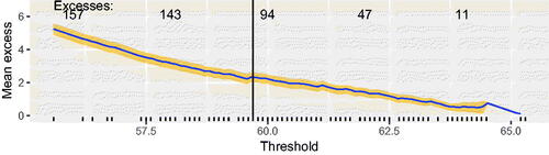
Figure 2 shows the calculated MRL plot. The solid line indicates the point estimate and the interval shows pointwise 95 percent confidence intervals. The vertical line at 59.7MPa indicates a potential lower bound for the threshold. Above this level, the plot shows fairly strict linearity, up to sampling variation. The pronounced negative gradient is a strong indication that the distribution of reverse collapse pressures has a short upper tail.

Figure 2. MRL plot for threshold selection, point estimates (solid line) and estimation uncertainty (shaded region). Bottom axis shows reverse collapse pressures (MPa). Top axis shows numbers of excesses of each threshold.

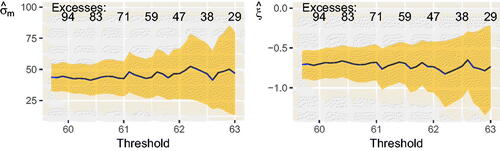
The threshold stability plots in Figure 3 show the parameter estimates are extremely stable over the range of thresholds examined. These plots show model parameters estimated using maximum likelihood, which is numerically efficient but can give poor estimates of uncertainty. The lowest threshold which we consider is that of 59.7 MPa, suggested by our MRL plot, above. The point estimates of the shape parameter ξ are well below zero. The tail behavior revealed in these and the MRL plots is inconsistent with the tails of a Normal model (since the Normal model has Exponential tails, we would anticipate ξ = 0 under this model).

Figure 3. Threshold stability plots for threshold selection, point estimates (solid line) and estimation uncertainty (shaded region). Bottom axis shows reverse collapse pressures (MPa). Top axis shows numbers of excesses of each threshold.

GPD model fitting

Having selected a suitable candidate threshold of 59.7 MPa, we look in more detail at the fit of the model at this threshold, and at sensitivity to threshold choice. This choice of threshold allows the largest possible number of threshold excesses to be used for estimation, and gives flexibility to increase the threshold if fit is found to be poor. For this threshold, we have 101 data points beyond the threshold which are used for estimation. The premise of EVT motivated statistical modeling is that information relevant to tail behavior lies in the tail of the data. So although we are discarding central data points, we retain all the information needed to model the tail and extrapolate to the levels of interest.

We use Bayesian MCMC methods to obtain posterior distributions of model parameters and derived quantities. We use a diffuse and uniformative Bivariate Normal prior on the parameter vector, with zero prior means, prior variances equal to 1e + 04 and zero prior correlation. All MCMC estimation is carried out by using a Metropolis Hastings algorithm, with chains run for 100,500 iterations, the first 500 being discarded as burn-in and the remaining 100,000 thinned to leave every 20th sample, to allow for the observed level of autocorrelation in the sampler output. Standard MCMC convergence diagnostics (not shown) were used to look for convergence issues and none were identified. Parameter estimates are illustrated in Table 1.

Table 1. Estimated model parameters for GPD fitted to reverse collapse pressures at a threshold of 59.7 MPa.

	Posterior mean	Posterior standard deviation
$\varphi$	1.366	0.116
ξ	−0.671	0.094

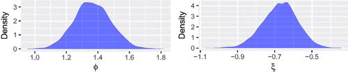
Figure 4 shows the posterior distributions of model parameters. These differ greatly from the uninformative priors, which are essentially flat on the scales plotted. The key parameter driving the tail shape is ξ. All posterior mass for ξ is well below 0 giving extremely strong evidence that the distribution of the underlying data is very short tailed.

Figure 4. Posterior distributions of model parameters, GPD fit to original reverse collapse pressure data. Plots show kernel density estimates of MCMC sampler output.

The diagnostic plots in Figure 5 show the good fit of the GPD to the data at this choice of threshold. The probability and quantile plots (top row) show sample versus theoretical quantiles, on different scales. Data points all lie within pointwise 95 percent prediction intervals. The return level plot is a standard diagnostic tool used to emphasize the extreme tail fit. It reveals the shape of the fitted tail: empirical (points) and model quantiles (fitted line) are expressed as return levels and plotted against associated return periods. The return period is the expected waiting time (number of independent observations) between excesses of the Return Level. Data points lie close to the line showing the fitted model, illustrating good model fit. The final plot in Figure 5 shows the fitted density, which matches closely the histogram of the data.

Figure 5. Diagnostic plots for GPD fit to original reverse collapse pressure data above a threshold of 59.7 MPa. The return period is the expected waiting time (number of independent observations) between excesses of the return level (MPa) shown on the vertical axis.

Diagnostics (not shown) for a range of thresholds from 59.7 to 61.7 MPa indicate that the quality of fit, and fit itself, are little affected by changes in threshold choice. Collapse pressure estimates are also affected very little by threshold choice in this range (see section on calculation of collapse pressures).

Normal model fit to collapse pressure data

Following Selker, Ramos, and Liu (2015), we fit the Normal distribution to the observed data. Fitted parameter values are: mean 39.2 MPa and standard deviation 2.1 MPa. Q–Q plots in Figure 1 show sample values plotted against the fitted Normal quantiles, for original and reverse pressure data. These plots show that the Normal model is not a poor fit to the data, as sample values lie within the prediction intervals. The Q–Q plots do not give strong evidence against the Normal model, but do show that the uppermost reverse collapse pressure observations do not follow exactly the line of equality. The diagonal line would form the basis of extrapolation of extreme quantiles under this model. The plots show that the upward growth of the largest reverse collapse pressures slows down compared with that of the Normal quantiles, above a reverse collapse pressure of around 63 MPa. Beyond this level, the observed tail shape is not closely matched by the tail of the fitted Normal model.

Other choices of statistical model

Extrapolation to pressures corresponding to the required very small probabilities is totally reliant on the choice of statistical model. We now consider another possible choice of statistical model in addition to the Normal and GPD. In the metocean industry, structural design criteria require extrapolation far into the tails of distributions of metocean variables, and it is common to compare fits from a range of distributions. Candidate models include GPD and Weibull distributions: the Weibull is often preferred since its exponentially decaying, unbounded tail can give realistic extrapolations where there is uncertainty about whether the underlying process has a finite endpoint (Dhanak and Xiros 2016).

We compare the Weibull distribution with the proposed GPD model (fit to all reverse collapse pressures above our threshold of 59.7 MPa) using diagnostic plots and formal goodness of fit tests such as Akaike Information Criterion (AIC) comparison. It is not possible to compare GPD and Normal fits in this way as these models are fit to different subsets of the data. Diagnostic plots (not shown) and AIC values show the GPD is a superior fit to the Weibull. For a threshold of 59.7 MPa (corresponding to fitting the models to 64 percent of the data), the AIC values were: GPD 344.9 and Weibull 355.8. A higher threshold of 62 improved the fit of the Weibull model, as judged by graphical diagnostics, but did not change our preference with AIC values of 114.7 (GPD) and 120.3 (Weibull). This is further strong evidence for the short-tailed nature of the collapse pressure data, and against the use of Normal or Weibull distributions which both have exponential type tails (data from these distributions have limiting GPD shape parameter ξ = 0).

Calculation of collapse pressures

We examine the effect of the following on the final collapse pressure estimates: threshold choice, the precise value of the single most extreme data point, and model choice.

Sensitivity checks

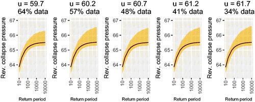
We estimate extreme quantiles of the fitted GPD using a range of threshold values. Figure 6 shows return level curves for each of these values. These plots show fits to the upper tail of the reverse collapse pressures distribution. Uncertainty associated with the estimated return level curves increases with estimation threshold, but the estimate itself is minimally affected by threshold choice.

Figure 6. Estimated quantiles and pointwise 95 percent credible intervals of reverse collapse pressure distribution, calculated for each of a range of threshold choices. The title of each plot shows the threshold u and the resulting proportion of data used for fitting at each choice of threshold. The horizontal axis shows the Return Period which is the expected waiting time (number of independent observations) between excesses of the level shown on the vertical axis.

We also examine the effect of the precise value of the smallest observed collapse pressure. We examine the impact of adding a single observation to the data set, lower than any observed collapse pressure. We re-fit the GPD model to the original data after the addition of a single point at 33.9 MPa and alternatively after the addition of a single point at 34.3 MPa. We use the original threshold of 59.7 MPa for all fitting. Adding these points does not materially change the character of the fitted tail. All posterior mass for ξ is concentrated away from zero. The original model fit (Figure 4) had the vast majority of mass on values of ξ less than −0.5, indicating an extremely short tail. Adding a single point at 34.3 MPa yields a greater proportion of mass on values above −0.5 (not shown), indicating a slightly lighter tail. Adding a single point further from the original data gives yet more mass assigned to values larger than −0.5 (also not shown), although there is still no mass assigned near 0. Our conclusions about tail behavior are therefore not changed by the addition of these points: the Normal model, which has exponential tails, is a poor description of the lower tail behavior of our data. We report results calculated under our alternative fitted models in the following section.

Estimated extreme quantiles of collapse pressure distribution

Tables 2 and 3 show estimates, with 95 percent credible intervals, of the following quantiles:

Table 2. Estimated lower quantiles and endpoint (MPa) for fitted collapse pressure distributions (all original data, with GPD model fitted at a range of thresholds).

Thresh =40.3 (0.64 quantile of data)		Thresh =39.3 (0.48 of data)	Thresh =38.3 (0.34 of data)
1e − 02	34.8 (34.3, 35)	34.8 (34.3, 35.1)	34.8 (34.3, 35.1)
1e − 03	34.6 (33.9, 34.7)	34.6 (33.7, 34.7)	34.5 (33.7, 34.7)
2e − 05	34.5 (33.6, 34.7)	34.5 (33.4, 34.7)	34.5 (33.2, 34.7)
1e − 07	34.5 (33.6, 34.7)	34.5 (33.4, 34.7)	34.5 (33.2, 34.7)
Endpoint	34.5 (33.6, 34.7)	34.5 (33.4, 34.7)	34.5 (33.2, 34.7)

Proportions of the original data lying beyond the fitting threshold, parentheses show 95 percent credible intervals.

Table 3. Estimated lower quantiles and endpoint (MPa) for fitted collapse pressure distributions (data supplemented by single point before GPD fitting, GPD threshold: 40.3 and Normal model fit to entire data set).

Quantile	Extra datum 34.3MPa	Extra datum 33.9MPa	Normal
1e − 02	34.5 (34, 34.8)	34.3 (33.6, 34.6)	34.2 (33.9, 34.5)
1e − 03	34.2 (33.3, 34.4)	33.8 (32.7, 34.1)	32.6 (32.2, 33)
2e − 05	34 (33, 34.3)	33.5 (32.2, 33.9)	30.4 (29.9, 30.9)
1e − 07	34 (33, 34.3)	33.5 (32.1, 33.9)	28.1 (27.5, 28.7)
Endpoint	34 (33, 34.3)	33.5 (32.1, 33.9)	NA (NA, NA)

Parentheses show 95 percent credible intervals.

• 0.01 quantile: 1 in 100 observations fall below this level. This is within our data range.

• 1e − 03 quantile: 1 in 1,000 observations fall below this level. Beyond our data range.

• 2e − 05 quantile: collapse probability 2e − 05, related to the number of pipe joints in the deepest water, that is, 50,000.

• 1e − 07 quantile: collapse probability 1e − 07, accords with DNVGL safety class very high.

• Endpoint: (for GPD with fitted negative shape parameter only; this does not exist for the Normal distribution) estimated minimum observable collapse pressure.

The lower endpoint of the fitted distribution is approached rather abruptly so that there is little physical difference between the estimated extreme quantiles. The GPD models fitted at the range of thresholds are the same to one decimal place. Quantile estimates are more sensitive to addition of points beyond the range of the data. This is hardly surprising, given that the two additional points considered both lie beyond estimated upper endpoint of the original distribution.

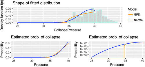
The estimated extreme lower quantiles calculated for the fitted Normal distribution are dramatically lower than those estimated by any of the GPD models. All of the point estimates of quantiles derived under the Normal model shown in Table 3 lie beyond the estimated lower endpoint derived under the GPD model. This shows that the tail behavior of the Normal distribution is totally incompatible with the shape revealed by the more flexible GPD family of models. The GPD family of models includes exponential tails – the tails of a Normal distribution – as a special case, and so if the Normal model was an adequate fit to these data then we would expect the extrapolation obtained under the fitted GPD and Normal models to agree, up to estimation uncertainty. Figure 7 highlights the difference between the Normal and GPD which have fundamentally different parametric forms and extrapolate very differently in spite of both appearing to fit the observed data tolerably well.

Figure 7. Comparison of fitted Normal and GPD densities, and impact on extreme quantile estimation.

Probability of pipe collapse on seabed

In the project described, the pipe was designed for placement at a seabed depth of 2,200 m and external pressure of approximately 22.3 MPa, when empty. The fitted GPD predicts a zero probability of pipe collapse at this depth. The Normal model predicts a 3e − 15 probability of occurrence. This suggests that the tested pipes would be in little danger of failure by collapse on the seabed.

The proposed method in practice

We now treat a number of practical questions which would need to be considered for the proposed procedure to be used in a practical setting.

Sample size considerations

We consider how many tests need to be carried out to prepare a test data base from which to determine the level of minimum collapse pressure with the necessary accuracy. Here, the estimation uncertainty will be influenced by a number of sources:

• Sample size (number of observations above threshold);

• The true underlying value of the shape parameter ξ;

• The true underlying value of the scale parameter σ_u;

• The accuracy of the GPD approximation to the underlying tail (this influences the threshold choice).

We give some guidelines for sample size choice in experimental design. We simulate from a GPD tail with given shape parameter ξ and scale parameter ${\sigma }_u=1$, and estimate GPD parameters and associated quantiles of the fitted tail for a range of sample sizes and values of ξ. We calculate relative error in the estimate ${\widehat{x}}_q$ of a true quantile x_q as $({\widehat{x}}_q-x_q)/x_q$. We explore a range of sample sizes and values of ξ. We avoid the need to explore different values of σ_u by reporting relative error in our calculations. We assume here that the GPD approximation is exact, in other words the threshold has been selected at a suitably extreme level for the GPD to give an exact representation of the tail behavior. In practice this would need to be examined by using the diagnostic tools illustrated above.

We generate 100 replicates of each experiment at each sample size/shape parameter combination and calculate the relative error for each replicate.

Figure 8 shows the mean relative error of our 100 replicates with pointwise 95 percent confidence intervals (estimated using the 0.025 and 0.975 quantiles of the corresponding 100 replicates). This figure shows the effect of sample size and the value of ξ on the estimation of extreme quantiles. For all fixed values of ξ, the effect of sample size is as anticipated, with accuracy increasing with the number of points lying beyond the threshold. However, the effect of ξ itself is marked with substantial decreases in accuracy as the underlying distribution becomes longer tailed (values of ξ closer to zero). This is true for all quantiles examined (the plots show relative error and so are comparable).

Figure 8. Relative error in estimate of collapse pressure with given probabilities of collapse, for different underlying shape parameter values and sample sizes n. Solid line indicates mean relative error and shaded region shows pointwise 95 percent confidence intervals, dashed line shows zero.

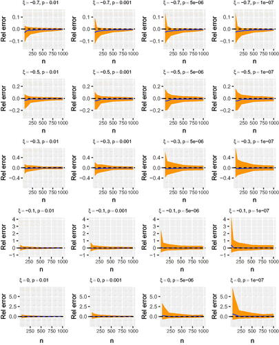
In the data application described here, the threshold excess sample size is 101 and the estimated value of ξ is −0.671. For such values of n and ξ, Figure 8 shows that the relative error of quantile estimates is typically less than 10 percent. Thus we benefit from the short tail exhibited by our sample. Data sets with heavier tails will have larger relative error and a bigger sample size would be needed to obtain a comparable level of accuracy.

Number of manufacture pipe joints in the project

The estimated distribution of collapse pressures describes the behavior of individual pipe sections. In a project, depending on the length of pipeline, there may be thousands – possibly tens of thousands – of pipe sections. Interest is in the probability of failure of the whole pipeline, in other words in the probability that at least one pipe section fails. This is straightforward to calculate from the fitted tail of the distribution of individual pipe collapse pressures under the assumption that the separate pipe sections behave independently of one and other. $\text{Pr}(N\text{section}\text{pipeline}\text{failure}\text{at}\text{pressure}X)$ is given by $1-\text{Pr}{(\text{Single}\text{pipe}\text{section}\text{does}\text{not}\text{fail}\text{at}\text{pressure}X)}^N$_, where the probability that a single section does not fail at pressure X is calculated using our approach for individual pipe collapse.

Discussion of results from statistical analysis

Figure 9 shows tail behavior for different values of ξ. Critical values of this parameter are:

Figure 9. Examples of densities of GPD lower tail models with different shape parameters. The location of the endpoint also depends on the scale parameter (not shown).

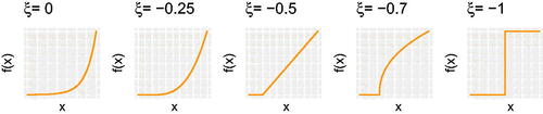
• $\xi >0$ heavy tails with polynomial tail decay, and an infinite endpoint;

• ξ = 0 exponential tails, and infinite endpoint;

• $-0.5<\xi <0$ light tails decaying to a finite endpoint, and concave density;

• $\xi =-0.5$ light tails decaying to a finite endpoint, and linear density;

• $\xi <-0.5$ light tails decaying to a finite endpoint, and convex density.

Our fitted collapse pressure distribution has $\widehat{\xi }=$−0.67, which explains the proximity of quantiles representing pressures with very different small probabilities of collapse.

Our approach has interesting implications for the minimum collapse pressure that would occur if many more tests were carried out. Under the Normal distribution assumption, as the number of tests is increased, the minimum observed pressure will reduce indefinitely. This contrasts with the short tail predicted by the GPD method, which suggests that no matter how many tests are carried out, the minimum observed collapse pressure will further reduce very little after a relatively small number of tests. In practice, an approximately constant minimum collapse pressure is likely to arise in the production process as a result of the inspection procedure which limits the minimum/maximum values of key variables controlling the collapse pressure in manufactured pipes. The short tail of the distribution revealed here is therefore more physically plausible and the GPD assessment of the minimum collapse pressure captures the effect of the pipe manufacture and inspection procedures.

The data set presented here is small compared with typical applications of EVT (see references in Introduction). In our application, the fitted tail is extremely short and super-efficiency of estimators works in our favor. The small sample size appears adequate for precise estimation of tail parameters and quantiles. In many applications of EVT motivated models, diagnostics support the use of (sometimes very) high quantiles as GPD fitting thresholds so that the vast majority of observations are excluded from GPD estimation. This is not the case in the current application where parameter and quantile estimates are robust threshold choice.

The estimated endpoint of our collapse pressure distribution is rather close to the lowest observed data point so that process control monitoring could in fact be rather straightforward. During testing of manufactured output, values observed beyond the estimated endpoint of the distribution (and certainly beyond the lower endpoint of the credible interval for this value) would be regarded as anomalous, and this may be an appropriate threshold to use to advise control procedures. The estimated low quantiles of this distribution lie close together, especially once estimation uncertainty is recognized, so that it may be pointless to attempt to distinguish between collapse pressures with probabilities of 2e − 05 and 1e − 07, since these estimated values are both very close to the estimated lower endpoint.

During manufacture, it would be straightforward to construct the set of k most recent measured collapse pressures of the manufactured product, and test for consistency between these and the observed distribution of collapse pressures obtained at the start of manufacture, or during experimental tests prior to production. Samples can be compared visually by using Q–Q plots such as that shown in Figure 5, or by using formal statistical testing of the null hypothesis that the underlying distributions are equal. Multiple testing will be an issue, and a significant result would be used to trigger further investigation rather than to conclude definitively about a problem with the manufacturing process.

We have compared an industry standard approach (Selker, Ramos, and Liu 2015, fitting and extrapolating under an assumed Normal distribution) with best practice from EVT motivated methods. We have illustrated that these two approaches give substantially different results for estimation of extreme quantiles. Our results give strong evidence that the Normal distribution is inappropriate for use in this setting, as its exponential lower tail does not describe well the true tail behavior of the data. We have shown that safety margins derived from current practice may be dramatically conservative. Our proposed method justifies rigorously the significant reduction of material and manufacturing costs, which would impact installation on a large scale for long distance pipe installation. Ring testing allows data to be collected in sufficient quantities to be used to assess the over-conservatism of the design method based on the DNVGL formulas. This has practical significance since there is a considerable financial penalty to be paid for increasing unnecessarily the wall thickness. Results from analysis of ring test data can be used to optimize pipe wall thickness and to balance safety and pipe manufacture costs. However, future deep water pipeline can only benefit if the method for assessing the collapse test results is appropriate and accurate.

Acknowledgments

The authors would like to thank VerdErg Pipe Technology Limited for commissioning the work which has resulted in the developments described in this article. We would also like to thank two anonymous referees for their constructive feedback which has substantially improved the presentation of our work.

Appendix

Data and R code for analysis

Original collapse pressure data (MPa): 40.4 39.4 39.7 41.6 40.5 40.9 41.5 42.4 39.5 38.5 38.4 38.4 38.4 35.8 36.2 37.9 37.0 37.1 37.9 34.7 36.8 37.2 38.6 39.0 39.5 39.4 38.9 39.5 38.1 38.1 37.8 38.5 38.3 36.8 37.8 36.7 37.6 38.4 39.3 40.6 40.1 39.8 39.8 35.8 36.1 36.1 37.3 36.0 40.3 41.2 40.4 40.4 40.4 43.6 42.1 42.6 41.5 41.0 41.1 38.0 38.0 40.1 39.2 39.4 41.1 42.0 42.1 42.5 41.4 37.5 36.5 36.7 36.7 36.9 35.5 35.5 36.0 37.3 38.5 36.2 35.6 38.1 37.2 36.2 35.6 36.3 36.0 37.3 34.7 40.1 39.1 41.2 37.1 38.9 34.8 35.9 36.0 35.7 36.7 40.3 40.1 39.9 38.9 38.9 44.4 43.8 43.3 42.1 43.2 39.2 42.4 41.7 40.4 41.1 40.4 40.9 40.9 41.2 41.7 40.4 41.1 40.4 40.9 40.9 41.2 39.4 39.3 39.5 40.8 41.4 40.4 38.7 38.9 39.6 40.8 40.2 39.0 39.7 39.8 39.3 41.7 40.2 40.0 43.2 41.2 38.9 38.9 41.9 38.1 37.8 38.4 40.4 41.9 37.7 37.9 37.3 40.3 42.2

The GPD fitting and diagnostic plots can be produced with the following lines of code. The 158 observed collapse pressures are held in the R object CPdat. Further information and guidance on using the R package texmex for extreme value analysis is given in the vignettes for this package.

library(texmex)trans <- function(x) -x + 100 # define transformationsrevTrans <- function(x) -(x - 100)revCP <- trans(CPdat) # calculate reverse collapse pressuresu <- 59.7 # thresholdgpd.fit <- evm(revCP,th = u, method="sim",thin = 20,iter = 100500) # fit GPD by using MCMCggplot(gpd.fit) # MCMC convergence diagnosticsggplot(gpd.fit$map) # GPD model fit diagnostics M <-c(10,20,50,100,200,500,1000,200010000)ggplot(predict(gpd.fit,M = M,ci.fit = TRUE)) # reproduce first plot inFigure 6M <- c(100, 1000, 20000, 10000000)p <- predict(gpd.fit, M = M,ci.fit =TRUE) # prediction on rev collapse pressure scale# transform back to original scale (note intervals are given with ends reversed!)lapply(p$obj,trans) # reproduces values inTable 2 column 1

References

- Anderson, C. W., G. Shi, H. V. Atkinson, C. M. Sellars, and J. R. Yates. 2003. Interrelationship between statistical methods for estimating the size of the maximum inclusion in clean steels. Acta Materialia 51 (8):2331–43.
- Coles, S. 2001. An introduction to statistical modeling of extreme values. London, UK: Springer.
- Davison, A. C., and R. L. Smith. 1990. Models for exceedances over high thresholds. Journal of the Royal Statistical Society. Series B (Methodological) 52 (3):393–442.
- Dhanak, M. R., and N. I. Xiros, eds. 2016. Springer handbook of ocean engineering. Cham: Springer.
- DNVGL Submarine Pipeline Systems. 2013. DNVGL OS F101.
- Finkenstadt, B., and H. Rootzèn, eds. 2003. Extreme values in finance, telecommunications, and the environment. Boca Raton, FL: CRC Press.
- Fougères, A.-L., S. Holm, and H. Rootzèn. 2006. Pitting corrosion: Comparison of treatments with extreme-value-distributed responses. Technometrics 48 (2):262–72.
- Gilks, W. R., S. Richardson, and D. Spiegelhalter, eds. 1995. Markov chain Monte Carlo in practice. Boca Raton, FL: CRC Press.
- Haigh, I. D., R. Nicholls, and N. Wells. 2010. A comparison of the main methods for estimating probabilities of extreme still water levels. Coastal Engineering 57 (9):838–49.
- Leadbetter, M. R., G. Lindgren, and H. Rootzén. 2012. Extremes and related properties of random sequences and processes. Dordrecht, Netherlands: Springer Science & Business Media.
- R Core Team. 2016. R: A language and environment for statistical computing. Vienna, Austria: R Foundation for Statistical Computing. https://protect-us.mimecast.com/s/s5SkC2kg95ip6oJmrInhljB?domain=r-project.org (accessed November 30, 2017)
- Selker, R., P. Ramos, and P. Liu. 2015. Interpretation of the South stream ring collapse test program results. International Journal of Offshore and Polar Engineering 25 (1):63–70.
- Slater, S., R. Devine, O. Aamlid, D. Hernandez, and D. Swanek. 2011. Qualification of enhanced collapse capacity UO deep water linepipe. Paper presented at Proceedings of the 36th International Conference on Ocean, Offshore & Arctic Engineering. American Society of Mechanical Engineers, Rotterdam, The Netherlands, June 19–24, 2011.
- Smith, R. L. 1987. Estimating tails of probability distributions. The Annals of Statistics 15 (3):1174–207.
- Southworth, H., J. E. Heffernan, and P. D. Metcalfe. 2016. Texmex: Statistical modelling of extreme values. https://cran.r-project.org/web/packages/texmex/citation.html. (accessed November 16, 2017)
- Tawn, J. A. 1992. Estimating probabilities of extreme sea-levels. Applied Statistics 41 (1):77–93.
- Walker, A., J. Chee, and P. Roberts. 2017. Assessment of thick-walled pipe for ultra-deep water pipelines. In Proceedings of ASME 36th International Conference on Ocean, Offshore and Arctic Engineering, ASME 2017-61083, Trondheim, Norway, June 25–30, 2017.