
 ?Mathematical formulae have been encoded as MathML and are displayed in this HTML version using MathJax in order to improve their display. Uncheck the box to turn MathJax off. This feature requires Javascript. Click on a formula to zoom.
Abstract
Acceptance sampling plans are used to determine whether production lots can be accepted or rejected. Existing tools only provide a limited functionality for the two-point design and the risk analysis of such plans. In this article, a web-based tool is presented to study single- and double-stage sampling plans. In contrast to existing solutions, the tool is an interactive applet that is freely available. Analytic properties are derived to support the development of search strategies for the design of double-stage sampling plans that are more efficient and accurate in comparison with existing routines. Several case studies are presented.
Introduction
Acceptance sampling is concerned with the design and implementation of sampling plans to inspect incoming or outgoing production lots. A typical application of acceptance sampling is the inspection by a company of a shipment of items from a supplier. These items are often components or raw material used in the company’s manufacturing process. A random sample is taken from the lot, and based on the inspection of some quality characteristic a decision is made to accept or reject the complete lot. The process of making this decision is also termed lot sentencing. Acceptance sampling plans can be classified according to the type of variables that are measured. Quality features that are measured on a numerical scale are used in variables sampling plans, while features that classify items as defective or non-defective lead to attributes sampling plans.
The use of acceptance sampling plans for inspection by attributes dates back to the seminal work of Dodge and Romig (Citation1941). The basic concepts and models of variables sampling plans were introduced by Jennett and Welch (Citation1939). During the past two decades of the 20th century, the research interest in acceptance sampling decreased. The use of acceptance sampling plans has been criticized as they are described as one-shot deals to test whether a production lot is conform to specifications without giving any feedback into either the production process or engineering design that would be necessarily for quality improvement (Montgomery Citation2013). However, acceptance sampling is still playing an important role in modern industrial environments and there has been a resurgence of interest in this field in the 21st century (Collani and Göb Citation2008). First, in many cases the producer has become increasingly removed from the consumer, not only by distance but also by language, culture and governmental differences (Schmueli Citation2016). There is a need for methods to keep generating pressure on suppliers in order that they maintain and improve the quality in their goods. Second, acceptance sampling plans are able to limit the risk for accepting lots of poor quality. In many applications the quality of incoming goods affect the efficiency of the production and the quality of the end product. For instance, for an egg processing company the freshness of the incoming eggs is essential to minimize drop-out during peeling of boiled eggs as will be discussed in more detail in case study II, presented later in this article. Other examples include the microbiological inspection of incoming goods in food industry for food safety and quality (Santos Fernãndez Citation2016). Finally, acceptance sampling can also be adapted to other verification problems as, for example, the verification of probabilistic design requirements using Monte Carlo simulation (White et al. Citation2009).
Single sampling plan (SSP) and double sampling plan (DSP) are among the most widely used acceptance sampling plans. In the procedure of an SSP plan a decision to accept or reject the lot is based on the result of one sample. The procedure of a DSP plan allows to take a second random sample from the lot when the information from the first sample raises too much doubt (Montgomery Citation2013). Sampling, however, involves the risk that the sample will not adequately represent an entire lot. There are two types of risk associated to each sampling plan: the producer’s (or supplier’s) risk and the consumer’s (or customer’s) risk. The producer’s risk reflects the probability to reject an acceptable lot that is defined as a lot with a proportion nonconforming of at most an acceptable quality level The customer’s risk reflects the probability to accept an unacceptable lot that is defined as a lot with a proportion nonconforming of at least a rejectable quality level
These risks are analytically studied by the operating characteristic (OC) curve which shows the probability of accepting a lot given various proportions nonconforming. A problem frequently encountered in quality control is the two-point design of a sampling plan where one is interested in the determination of sampling plans that reduce the producer’s and consumer’s risk below some predefined levels α and β, respectively (Taylor Citation1997). For this reason, several tables have been presented in the literature to select sampling plans (Duarte and Saraiva Citation2013; Sommers Citation1981). Commonly used tables are included in international standards as the ISO standards (and their ANSI/ASQC/BS or other counterparts (Neubauer and Luko Citation2012, Citation2013)). Such tables, however, are restricted to a limited number of values for
α and β and are not accompanied with user-friendly tools to evaluate the individual sampling plans regarding the risks associated with sampling error.
Furthermore, a limited number of computer programs are available to study sampling plans and only few offer the ability to design DSP as well as SSP plans. Commercial programs, for example, Minitab, Inc. (2018), only allow the two-point design of an SSP plan. Also, easy-to-use Excel sheets are available to study SSP plans (Bertoni Citation2016). Kiermeier (Citation2008) developed an R-package ‘Acceptance Sampling’ that allows to calculate OC-curves of SSP and DSP plans, but the functionality of a two-point design is limited to that of an SSP plan. Furthermore, Cheng and Chen (Citation2007) developed a computer program that is based on an evolutionary algorithm (Zelinka Citation2015) to design attributes DSP plans. Its interface, however, requires the interpretation of several parameters and its implementation is outdated.
The design of two-point sampling plans with an OC-curve that passes approximately through two designated points and
can be described by a system of algebraic equations. Since such system does not have a closed from solution for SSP and DSP plans, algorithms have been developed to search for feasible combinations of the parameters of the plan that ensure a producer’s and consumer’s risk below the predefined levels α and β, respectively. Existing routines to design two-point sampling plans can be classified into two main approaches: (i) search routines that perform an exhaustive search to find appropriate combinations of the parameters of a two-point sampling plan and (ii) optimization procedures where some cost function (e.g. the sample size or average sample number (ASN)) is minimized subject to the constraints induced by the two-point method. Optimization procedures have the advantage to be applicable to other types of sampling plans, for example, multiple dependent sampling plans (Balamurali and Jun Citation2007). However, convergence may not be guaranteed with such approaches and finding appropriate starting values may not be evident for the user (Balamurali and Usha Citation2013; Duarte and Saraiva Citation2013). The focus in this article is on search routines that do not depend on starting values and whose implementation will lead to a user-friendly tool to design and analyze DSP plans as well as SSP plans.
Early development of search routines for the design of sampling plans were performed with the programing language FORTRAN (Chow et al. Citation1972; Hailey Citation1980). A general algorithm to develop two-point SSP plans for inspection by attributes was introduced by Hailey (Citation1980). For variables SSP plans computational formulas are available (Schilling and Neubauer Citation2009). The two-point design of DSP plans, however, is more complex as more parameters are involved (two sample sizes n1 and n2 and two acceptance numbers c1 and c2 to test sample results). To reduce the number of possible combinations of parameters, a fixed relationship between the sample sizes n1 and n2 is often assumed. The most common constraint that has been used is to require that n2 is a multiple of n1, that is, (Montgomery Citation2013). For attributes inspection, previous developed search routines have assumed a Poisson distribution (Chow et al. Citation1972). In addition, additional constraints on the acceptance numbers (c1, c2) have been studied, for example,
or
(Newman and Yu Citation2018; Olorunniwo and Salas Citation1982; Vijayaraghavan Citation2007). For variables inspection, Sommers (Citation1981) has developed a table of DSP plans with a minimum ASN at
Unique DSP plans have been obtained by minimizing other cost functions as well, for example, the maximum ASN (Krumbholz and Rohr Citation2009; Vangjeli Citation2012).
In this article, we develop search routines for the design of attributes and variables DSP plans that minimize the ASN at For this purpose, it is assumed that n2 is a multiple of n1. Analytic properties of DSP plans are derived that are given a mathematical proof and that will support the development of the search routines. For attributes inspection, the number of nonconforming items in a lot is modeled by a binomial distribution. It is shown that several constraints hold on the parameters of an attributes DSP plan reducing the number of possible combinations of parameters that have to be considered during an exhaustive search routine (Olorunniwo and Salas Citation1982). For variables inspection, the measurement data are modeled using a normal distribution with known standard deviation σ. The search routine to design variables DSP plans is shown to result in more accurate minimum values of the ASN when compared to the routines introduced by Sommers (Citation1981). Furthermore, search routines are implemented in a user-friendly and interactive web tool to design and analyze SSP and DSP plans. Unlike previous developed solutions, the tool is an interactive applet that is easy and freely accessible and that supports the two-point design of DSP plans for inspection by attributes as well as variables. Several case studies from food industry are discussed to illustrate the use of the tool.
Note that the study of variables inspection plans is restricted to the case where one specification limit is defined and where measurements are drawn from a normal distribution with known variance. Extensions of the properties and design to the case of double specification limits or to the case where quality features are studied that follow other probability distributions (e.g., an exponential distribution) can be a subject of further research. The remainder of the article is structured as follows. Firstly, the reader is introduced to the necessary terminology and notations of acceptance sampling. Subsequently, several analytic properties of the OC-curves of DSP plans are derived. Moreover, search routines to develop two-point DSP plans are presented. Next, these routines, together with procedures to design SSP plans, are implemented in a web-based tool that is illustrated by several case studies. Finally, a conclusion is made.
Background on acceptance sampling
Firstly, an introduction is given to the risk analysis of acceptance sampling plans using OC-curves. Next, a general background on SSP and DSP plans is given.
Risk analysis and OC-curves
Sampling plans are subject to sampling error and therefore induce risks. A fundamental tool to describe the risks associated to a sampling plan is the OC-curve
which relates the proportion nonconforming present in the lot to the probability of acceptance of a lot using the plan
The statistical design of a sampling plan is based on two specific points on the OC-curve:
The producer’s risk point denoted as
The acceptable quality level
The consumer’s risk point denoted as
Ideally the quality engineer would like to set to design a sampling plan that would accept all lots with
and reject all lots with
However, such ideal plan can only be realized by 100% inspection, if the inspection would be error-free. Therefore, one sets
and a sampling plan is designed such that the OC-curve passes approximately through the points
and
[1]
[1]
The ideal OC-curve of a 100% inspection plan can be approached by increasing the sample size(s) of the sampling plan. The slope of the OC-curve is a measure for the discriminating power of the plan. In the next section, we will illustrate these principles on SSP and DSP plans.
Single sampling plans
An SSP plan for inspection by attributes is a procedure in which a decision is made to accept or reject a lot of size N based on the number of nonconforming items of a random sample of size n < N taken from it. Such a sampling plan is defined by two integers (n, c), with c < n, and where n denotes the sample size and c denotes the maximal number of nonconforming items c that are allowed in order to accept the lot under inspection (the so-called acceptance number).
When the lot size is large (), the number of nonconforming items D that is found in samples of size n drawn from the lot follows approximately a binomial distribution, that is,
where p denotes an (unknown) lot fraction nonconforming p. The OC-curve
of an SSP-(n, c) plan is given by:
[2]
[2]
and a statistical design is a solution of the system of EquationEq. [1]
[1]
[1] that is given by:
[3]
[3]
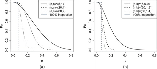
shows how the OC-curves of attributes SSP plans change when the sample size n and the acceptance number c change. The OC-curve becomes more like the idealized OC-curve when the sample size n increases. Plans with a lower acceptance number c provide more discriminating power at lower proportions nonconforming. Minimal sample sizes can be achieved by considering zero acceptance number sampling plans (Hahn Citation1974).
Figure 1. OC-curves of several sampling plans where Pa denotes the acceptance probability: (a) attributes sampling plans and (b) variables sampling plans. The idealized OC-curves corresponding with complete inspection are shown in gray.
When a continuous variable X in a lot of size N is inspected, one can use an SSP plan for inspection by variables. Such plan assumes that the variable X follows a normal distribution with mean μ and a known standard deviation σ. When an upper-specification limit U on the variable X is defined, a single lot is accepted under the condition
where k is a continuous acceptance constant indicating the minimal standardized distance between the sample mean
and the upper-specification limit U. Similarly, when a lower-specification limit L is used, the condition is given by
In both cases the OC-curve for a variables SSP-(n, k) plan is defined by:
[4]
[4]
where
and
denotes the cumulative distribution function of a variable Z following a standard normal distribution N(0, 1).
shows how the OC-curves of variables SSP plans change as the sample size n and the acceptance constant k change. A higher acceptance constant implies a higher discriminative power at lower proportions nonconforming. Larger sample sizes result in a better protection of producers and consumers and lead to OC-curves that become more like the idealized OC-curve.
In case the measurements show a strong deviation from normality, cautionary is required in applying formula Equation[4][4]
[4] . Alternative variables SSP
plans exist for exponential, gamma and Weibull distributions. An overview is given by White and Johnson (Citation2013).
Double sampling plans
A DSP plan allows to take a second random sample when the information from the first sample raises to much doubt about the decision whether to accept or reject the lot. When a second sample is taken, the information from the first and second sample is combined in order to decide whether to accept or reject the lot.
Following Montgomery (Citation2013), a DSP plan for attributes inspection is defined by four parameters with
and operates as follows:
Stage I. A random sample of size n1 is taken from the lot. If the number of nonconforming items D1 that is found in the first sample does not exceed the first sample acceptance number c1, the lot is accepted; If D1 exceeds the second sample acceptance number c2, the lot is rejected.
Stage II. If
The OC-curve of a DSP- plan is given by:
[5]
[5]
In contrast to an SSP plan, the total number of inspected items is not constant, but depends on the number of nonconforming items found in the first sample. The probability of drawing a second sample varies with the proportion nonconforming that determines the ASN. The ASN of a DSP plan is determined by:
[6]
[6]
where PI is the probability that the lot is accepted or rejected on the first sample, that is,
The ASN curve shows the ASN as a function of the lot fraction nonconforming p.
For variables inspection, we follow Sommers (Citation1981) and define a DSP plan by four parameters with
and with the following operating procedure:
Stage I. A random sample of size n1 is taken from the lot. When the standardized difference between the sample mean and the lower (or upper) specification limit, that is,
Stage II. When
The OC-curve of a DSP- plan is given by:
[7]
[7]
where
and P2 is a cumulative probability associated to a bivariate normal distribution
with:
[8]
[8]
and
[9]
[9]
The dependency between the variables W1 and W2 in the expression of is due to the dependency of the result in the second stage and the result in the first stage. Indeed, the decision in the second stage is based on
and therefore depends on the result of the sample taken in the first stage (Sommers Citation1981).
The expression for the ASN curve is based on Equation[6][6]
[6] . The probability PI is now given by:
[10]
[10]
Search procedures for double sampling plans
In this section, we provide the reader with algorithms to design DSP plans. A statistical design relies on a solution of the system of EquationEq. [1][1]
[1] that ensures that the OC-curve passes approximately through the two points
and
As the parameters of DSP plans are non-negative integers, one can rely on mixed integer non-linear programing techniques. However, convergence may not be guaranteed by such approaches and finding appropriate starting values may not be evident for the user (Duarte and Saraiva Citation2013). Alternatively, routines can be developed that list all possible parameter combinations of DSP plans that solve Equation[1]
[1]
[1] . To keep the computation time limited, an additional constraint is chosen on the sample sizes of the plans requiring that n2 is a multiple of n1. A unique sampling plan is returned by minimizing the ASN at
Design of two-point attributes double sampling plans
Let us first recall some properties of the design of an SSP-(n, c) plan. Geometrically, a two-point SSP-(n, c) plan with an OC-curve that approximately passes through the points and
will be situated in a region of the nc-plane consisting of all the points (n, c) that satisfy
with:
[11]
[11]
and where nl and nu are non-decreasing as a function of c. If
there does not exist a two-point SSP-(n, c) plan for the points
and
In what follows,
denotes the minimal acceptance number such that
Setting
leads to the two-point SSP-
plan with minimum sample size
(Luca Citation2018).
In the following property, the effect is studied of changes in sample sizes or acceptance numbers on the OC-curve of a two-point DSP- plan. A proof is given in Appendix A. The property will support the development of an efficient search procedure for the design of a two-point DSP plan.
Property 1.
Consider a DSP- plan and it’s corresponding OC-curve:
The OC-curve of a DSP-
In particular, if
Consider the SSP-
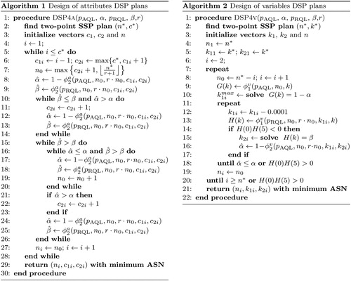
In Algorithm 1, we present the pseudo-code of a search procedure for a two-point DSP- plan with
(
) and with a minimum ASN such that the OC-curve passes through two specified points
and
The first step in designing a two-point attributes DSP-
plan is to search the corresponding SSP-
plan with an OC-curve that passes through the two points
and
From Property 1 (iv), it follows that an exhaustive search on the parameters
can be restricted to acceptance numbers (c1, c2) satisfying
The latter restriction leads to a more efficient search when compared to existing procedures that test every combination of the acceptance numbers c1 and c2 (Olorunniwo and Salas Citation1982). Furthermore, because
one finds
such that
The search strategy of Algorithm 1 (see ) calculates for each first sample acceptance number a corresponding second sample acceptance number
and sample sizes
that are required to assure that as well the producers as the consumers are protected. For a given c1, one starts with initialization by considering the sampling plan with n1 and c2 as small as possible. When
and
the while loops between line 10 and line 26 are not entered and the sampling plan
is chosen. When the consumer’s risk is lower than the requested limit β and the producer’s risk is higher than α, an increase of the acceptance number c2 is considered (which increases the consumer’s risk but lowers the producer’s risk due to Property 1(i)) while keeping the sample size as low as possible (such that the producer’s risk is at its minimum) until the producer’s risk is lower than α or the customer’s risk exceeds β. At the end of the while loop starting at rule 10 of Algorithm 1, either
and
leading to the desired sampling plan or
In the latter, one enters the while loop at rule 15 where the sample size is increased when the producer’s risk is lower than α (Property 1(ii)). At rule 20 the desired plan is found or
such that the acceptance number c2 has to be increased to reduce the producer’s risk. The while loop that started at line 15 continues when
Next, c1 is increased and the while loop over i that started at line 5 restarts a next iteration.
Figure 2. Algorithms for the design of two-point DSP plans. The parameters of the procedures determine the producer’s and consumer’s risk point. A constraint on the sample sizes can be chosen by specifying
At the end, the procedure has calculated a series of DSP- plans with
and
and with OC-curves that pass through the two points
and
Using EquationEq. [6]
[6]
[6] , the sampling plan with the minimum ASN can be returned.
Remark that Algorithm 1 can be adapted to the hypergeometric case where the lot size N is an additional parameter. Indeed, the dependency on the sample sizes and criteria of the acceptance probability related to a hypergeometric distribution is similar to the dependency on the sample sizes and criteria of the acceptance probability of a binomial distribution such that Property 1 will also hold for the hypergeometric case. Furthermore, other constraints on the sample sizes can be considered by replacing in Algorithm 1 by another function f.
Design of two-point variables double sampling plans
The following property studies the effect of the changes in the parameters of a two-point variables DSP- plan on its OC-curve. Due to the scalar nature of the criteria (k1, k2), the proof of Property 2 requires a different reasoning than the proof of Property 1 (see Appendix A).
Property 2.
Consider a variables DSP- plan and it’s corresponding OC-curve:
There exist
The OC-curve of a DSP-
If k1 = k2, the DSP-
Consider the SSP-
The procedure to calculate a DSP plan for variables inspection is given in Algorithm 2. As with attributes inspection, the procedure starts with the design of an SSP- plan with an OC-curve that passes through two points
and
such that
becomes an upper bound of n1 (Property 2(iv)). For each
criteria (k1, k2) are calculated that guarantee a producer’s risk and a consumer’s risk of at most α and β, respectively. For this purpose, an SSP-
plan is calculated to find an upper bound on k1 that corresponds to a producer’s risk α (Property 2(ii)). Consequently, a grid search is performed to find appropriate values for k1 and k2 in the repeat loop starting at rule 7. By lowering k1, the consumer’s risk increases which can be compensated by an increase in k2 such that the consumer’s risk is at most β (Property 2(i)). At the same time, it is checked whether the producer’s risk stays below α. When n1 is chosen too low, the consumer’s risk will be too high and no solution won’t be found for
such that the loop terminates (Property 2(ii)). Choosing a range of
for k2 enables to find solutions for a wide range of values for the parameters of DSP plans (see Table B1 in Appendix B). Finally, the plan is returned with the minimum ASN by use of Equation[6]
[6]
[6] and Equation[10]
[10]
[10] .
Tabulated single and double sampling plans
To illustrate the use of Algorithms 1 and 2, we present a table of matching SSP and DSP plans for variables and attributes inspection in Appendix B. The SSP plans are calculated using the search routines described by Kiermeier (Citation2008). The DSP plans are calculated by minimizing the ASN at The plans are matched such that the OC-curves pass through the two points
and
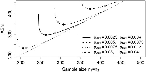
The DSP plans for inspection by variables are defined following the principles of Sommers (Citation1981). In contrast to the procedure proposed by Sommers (Citation1981), the use of Algorithm 2 resulted in more accurate minima of the ASN at To illustrate this, shows the ASN at
as a function of the sample size n1 = n2 of the DSP-
plans that pass through the two points
and
The curves correspond to several choices of
and
The gray dots indicate the plans tabulated by Sommers (Citation1981), while the black dots indicate the plans obtained by using Algorithm 2. Clearly, the use of Algorithm 2 results in sample sizes that correspond more accurately to a minimum of the ASN curve.
Figure 3. The ASN at as a function of the sample size n1 = n2 for several two-point DSP-
plans that pass through two points
and
The dotted identity line correspond to an SSP-(n1, k1) where ASN
The gray and black dots correspond to the plans obtained by Sommers (Citation1981) and Algorithm 2, respectively.
A web tool to design and study sampling plans
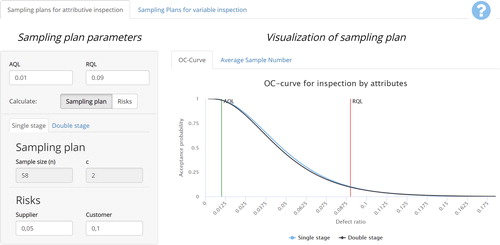
In this section a web tool is presented to develop and study SSP and DSP plans. The web tool is available at https://www.acceptancesampling.com/ and aims at providing a user-friendly way to develop and analyze two-point sampling plans. The tool is organized in two sheets: one sheet for attributes inspection and one sheet for variables inspection (). Routines underlying the statistical computations were implemented in R (R Core Team Citation2018). The web interface is based on the PHP-language and the HTML-library bootstrap (Duckett Citation2014; Spurlock Citation2013). The use of four different types of sampling plans was implemented:
Figure 4. The interface of our web tool that consists of a left panel to set the sampling plan parameters and a right panel to visualize the plan with an OC-curve and an ASN curve. The selection of the main sheet determines the type of inspection: attributes inspection or variables inspection. The left panel allows to implement single-stage and double-stage sampling plans.
SSP plans for inspection by attributes based on the binomial distribution.
SSP plans for inspection by variables based on a normal distribution with a known standard deviation σ.
DSP plans for inspection by attributes based on the binomial distribution.
DSP plans for inspection by variables based on a normal distribution with a known standard deviation σ.
Each sheet consists of a left and a right panel of which the structure and functionality are very similar across the different types of plans to enhance user-friendliness.
Introducing the panels of the web tool
The interface consists of a left panel that shows the parameters of a plan and a right panel that visualizes a plan by the OC-curve or the ASN curve (). In particular, the left panel shows the sample sizes and relevant criteria of the sampling plan together with the risks related to sampling error. To increase the ease of interpretability for practitioners the terms supplier’s risk and customer’s risk are used. A typical application of the tool is the inspection by a company (the customer) of an incoming lot from a supplier. Furthermore, the quality levels can be specified: the acceptable quality level, abbreviated as AQL and the rejectable quality level, abbreviated as RQL. A help page is available at the top right corner to introduce the user to the functionality of the tool and the terminology that is used.
The use of the left panel is implemented in two directions: (i) one can calculate a sampling plan given the parameters and
or (ii) the risks α and β are calculated given the sampling plan and the quality levels
and
The sampling plans are obtained by an implementation of Algorithms 1 and 2. Risks can be calculated using formulas Equation[2]
[2]
[2] , Equation[4]
[4]
[4] , Equation[5]
[5]
[5] , Equation[7]
[7]
[7] , and Equation[9]
[9]
[9] .
The layout of the left panel depends on the type of sampling plan (). For a variables SSP-(n, k) plan, lot acceptance can also be described by an upper bound M on an unbiased estimate of the lot fraction nonconforming (the so-called M-method). When the standard deviation is known, this upper bound may be found by for
(Schilling and Neubauer Citation2009).
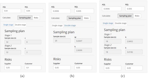
Figure 5. Left panels of the interface: (a) the parameters of a DSP- plan for inspection by attributes, (b) the parameters of an SSP-(n, k) plan for inspection by variables, and (c) the parameters of a DSP-
for inspection by variables. The panel in (a) is part of the main sheet entitled sampling plans for attributes inspection as shown in . The panels in (b) and (c) are part of the main sheet entitled sampling plans for variables inspection.
When the sampling plans at the left panel are entered, the right panel visualizes the plan by an OC-curve or a plot of the ASN as a function of the lot fraction nonconforming. As well the acceptable quality level as the rejectable quality level
are indicated on the OC-curve by vertical lines. The acceptance probability at
should be approximately
the acceptance probability at
should be approximately the customer’s risk β. The ASN curves are calculated using formulas Equation[6]
[6]
[6] and Equation[10]
[10]
[10] . For the SSP plans, the ASN curve will be given by a horizontal line. For a DSP plan, the lots will usually be accepted in the first stage when the quality is very good and rejected in the first stage when the quality is very bad. When lots are of intermediate quality, a second sample will be required and the total number of items that need to be inspected will increase.
Case studies
We discuss three case studies at three different companies that are active in the food industry: (i) an apple juice company, (ii) a cheese company, and (iii) a company that processes eggs.
Case study I
An apple juice company inspects a lot of 150,000 apples. Each lot is conforming or nonconforming towards the amount of rotten apples (an apple is rotten when patulin is present). The company uses an SSP plan by attributes with sample size n = 50 and an acceptance number c = 2 and is interested whether a DSP plan is more appealing concerning average inspection effort.
The company has agreed with local farmers to set the acceptable quality level to 1% and the rejectable quality level to
The company is interested in an answer on the following questions:
What is the supplier’s and customer’s risk of the SSP-(50, 2) plan?
Which two-point SSP plan corresponds to a supplier’s and customer’s risk of 5 and 10%, respectively?
Which corresponding two-point DSP plan can be used and will this plan lead to a decrease of the ASN at an operating proportion nonconforming of
To answer question 1, the left panel of the attributes inspection sheet can be used. The supplier’s risk and customer’s risks of the operating attributes SSP-(50, 2) plan are returned as 1.38 and 16.05%, respectively after entering the sampling plan parameters. Switching to the calculation of an SSP (), the web tool advices an SSP-(58, 2) answering question 2. For a DSP plan, sample sizes and criteria
are advised (). An ASN of approximately 41 is returned by reading the value of the ASN curve (complete inspection) corresponding to
Case study II
An outgoing shipment of 2500 pieces of cheese is inspected. The pH of such a shipment should be at most U = 7.00. The quality levels and
are set to 0.06% (6 out of 10,000) and 0.5%, respectively. The company is interested in the following questions:
Which two-point SSP and DSP plan is appropriate to limit producer’s and customer’s risk to 5%?
What is the maximum sampling effort that can be expected when the DSP plan is used?
shows how to obtain the desired SSP and DSP plan, respectively. For an SSP plan, a sample size of n = 25 and an acceptance constant k = 2.91 is advised. Equivalently, an estimation of the lot fraction nonconforming should be below in order to accept the lot. For a DSP plan, the sample sizes are given by
and the criteria in the first and second stage are given by
and
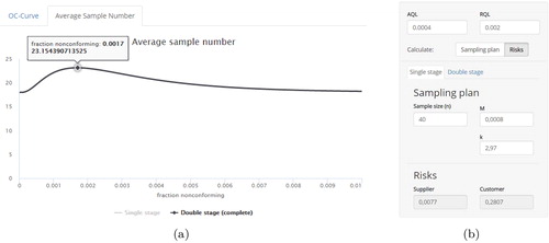
respectively. The corresponding ASN curve shows a maximum sample size of approximately 23 at
which gives an indication of the maximum sampling effort that can be expected ().
Figure 6. (a) The ASN curve of a DSP- for variables inspection. (b) The risks associated to an individual ISO 3951-1 SSP-
plan for inspection by variables.
Case study III
A food company that is specialized in egg processing daily receives multiple shipments of eggs that are being cooked and peeled. The freshness of the eggs is essential to minimize drop-out during peeling. For this purpose, the Haugh unit is measured, which is a measure of egg protein quality that is based on the height of the thick albumen (egg white) that immediately surrounds the yolk. Testing is destructive as the Haugh unit can only be measured by breaking the egg. The frequency of shipments is 4 per day where each lot consists of 324,000 eggs. The company and supplier who delivers the eggs agree to set the quality levels and
as 0.04 and 0.2%, respectively. The supplier’s and customer’s risk are set to 5 and 10%, respectively. A lower specification limit of L = 65 is set to the measured Haugh unit.
The use of the tables of the ISO 3951-1 results in an SSP- (standard inspection level II, σ-method). Associated supplier’s and customer’s risk are given by 0.77 and 28.07%, respectively (). The focal point of the ISO 3951-1 standard is the acceptable quality level which ranges from 0.01% to 10%. To control the customer’s risk up to a certain level, three general levels are available. The use of level III results in a sample size of n = 50 and an acceptance constant of k = 3.01 and reduces the customer’s risk to 17.56%. However, by use of the web tool one can achieve a two-point SSP-
plan corresponding to a supplier’s and customer’s risk not exceeding 5 and 10%, respectively. Alternatively, a matching two-point DSP-
can be used.
Conclusion
In this article, we introduced novel search routines for the design of DSP plans for inspection by attributes and variables. Analytic properties of DSP plans were derived that were given a mathematical proof. We found that several constraints hold on the sample sizes and the criteria of two-point attributes DSP plans leading to a more efficient search routine compared to existing ones. For variables DSP plans, a routine was developed that lead to more accurate sample sizes when compared to existing tables and routines.
Furthermore, we introduced and discussed a user-friendly and interactive web tool to design and analyze SSP and DSP plans and that is freely available at www.acceptancesampling.com. In comparison with existing solutions the tool is an interactive applet that supports a two-point design of DSP plans as well as SSP plans. The use of the web tool was demonstrated on several case studies. In comparison with international standards the tool can be used to obtain a statistical interpretation of the sampling plans in terms of the consumer’s and the producer’s risks.
Several interesting future research directions are possible. First, extensions of our search routines to the design of sampling plans with more than two stages can be studied. Second, the design of variables DSP plans can be extended to the case of unknown variance or double specification limits. Third, algorithms can be developed that are independent of constraints on the sample sizes n1 and n2.
About the authors
Stijn Luca holds a MSc in Mathematics from KU Leuven (Belgium, 2003) and a PhD in mathematics from Hasselt University (Belgium, 2007). Currently, he is an assistant professor at the Department of Data Analysis and Mathematical Modelling of the Faculty of Bioscience Engineering at Ghent University (Belgium). Previously, he was a postdoctoral fellow at KU Leuven (Belgium) and a visiting scholar at the University of Oxford (2014–2015). Luca’s research interests surround the theory and methods of statistical data analysis and its applications.
Johan Vandercappellen obtained a MSc in Bio-engineering from KU Leuven and postgraduates in Quality Management and ICT from UHasselt. He is founding manager of VDC Consulting bvba, a successful consultancy company in the domain of quality management consulting and of Quasydoc a SAAS application for Quality Management in food production plants both situated at Hasselt, Belgium. He has more than 30 years of experience in quality management for companies including Mora NV (Unilever), Konings NV, Irish Dairy Board. Besides, he is a lector in quality assurance and food safety management at university college PXL.
Johan Claes is professor in food engineering at the Department of Microbial and Molecular Systems (KU Leuven). He obtained his M.Sc. in Food Technology and a PhD in Bio-Engineering from KU Leuven. After finishing his PhD, he became program coordinator of the Master in Biosciences, Food Technology and started the research group Lab4Food both at Campus Geel of KU Leuven. His main research area is food texture, rheology and sensory analysis. In addition, he is also consulting food companies about food quality systems and legislation.
References
- Adams, R., and C. Essex. 2009. Calculus: A complete course. 7th ed. Canada: Pearson Education.
- Balamurali, S., and C.-H. Jun. 2007. Multiple dependent state sampling plans for lot acceptance based on measurement data. European Journal of Operational Research 180 (3):1221–30. doi: 10.1016/j.ejor.2006.05.025.
- Balamurali, S., and M. Usha. 2013. Optimal designing of variables chain sampling plan by minimizing the average sample number. International Journal of Manufacturing Engineering 2013:1–12. doi: 10.1155/2013/751807.
- Bertoni, C. 2016. Sample simplification. Quality Progress 8:23–7.
- Cheng, T.-M., and Y.-L. Chen. 2007. A GA mechanism for optimizing the design of attribute double sampling plan. Automation in Construction 16 (3):345–53. doi: 10.1016/j.autcon.2006.07.003.
- Chow, B., P. Dickinson, and H. Hughes. 1972. A computer program for the solution of double sampling plans. Journal of Quality Technology 4 (4):205–9. doi: 10.1080/00224065.1972.11980552.
- Collani, E. V., and R. Göb. 2008. Acceptance sampling in modern industrial environments. In Encyclopedia of statistics in quality and reliability, eds. F. Ruggeri, R. Kenett, and F. Falting. Hoboken, NJ: John Wiley & Sons.
- Dodge, H., and H. Romig. 1941. Single sampling and double inspection tables. Bell System Technical Journal 20 (1):1–61. doi: 10.1002/j.1538-7305.1941.tb00851.x.
- Duarte, B., and P. Saraiva. 2013. An optimization-based framework for designing acceptance sampling plans by variables for non-conforming proportions. International Journal of Quality & Reliability Management 27 (7):794–814. doi: 10.1108/02656711011062390.
- Duckett, J. 2014. Web design with HTML, CSS, JavaScript and jQuery set. IN: Wiley.
- Hahn, G. 1974. Minimum size sampling plans. Journal of Quality Technology 6 (3):121–7. doi: 10.1080/00224065.1974.11980633.
- Hailey, W. 1980. Minimum sample size single sampling plans: A computerized approach. Journal of Quality Technology 12 (4):230–5. doi: 10.1080/00224065.1980.11980970.
- Jennett, W., and B. Welch. 1939. The control of proportion defective as judged by a single quality characteristic varying on a continuous scale. Supplement to the Journal of the Royal Statistical Society 6 (1):80–8. doi: 10.2307/2983626.
- Kiermeier, A. 2008. Visualizing and assessing acceptance sampling plans: The R package acceptance sampling. Journal of Statistical Software 26 (6):1–20. doi: 10.18637/jss.v026.i06.
- Krumbholz, W., and A. Rohr. 2009. Double ASN minimax sampling plans by variables when the standard deviation is unknown. Asta Advances in Statistical Analysis 93 (3):281–94. doi: 10.1007/s10182-009-0111-8.
- Luca, S. 2018. Modified chain sampling plans for lot inspection by variables and attributes. Journal of Applied Statistics 45 (8):1447–64. doi: 10.1080/02664763.2017.1375084.
- Minitab, I. 2018. Minitab 18 statistical software. www.minitab.com.
- Montgomery, D. C. 2013. Introduction to statistical quality control. 7th ed. USA: John Wiley & Sons.
- Neubauer, D., and S. Luko. 2012. Comparing acceptance sampling standards, part 1. Quality Engineering 25 (1):73–7. doi: 10.1080/08982112.2013.738146.
- Neubauer, D., and S. Luko. 2013. Comparing acceptance sampling standards, part 2. Quality Engineering 25 (2):181–7. doi: 10.1080/08982112.2013.758557.
- Newman, R., and S. Yu. 2018. An alternative approach to accept on zero and accept on one sampling plans. Quality Engineering 30 (2):183–94. doi: 10.1080/08982112.2017.1328064.
- Olorunniwo, F., and J. Salas. 1982. An algorithm for determining double attribute sampling plans. Journal of Quality Technology 14 (3):166–71. doi: 10.1080/00224065.1982.11978810.
- R Core Team. 2018. R: A language and environment for statistical computing. Vienna, Austria: R Foundation for Statistical Computing.
- Santos Fernãndez, E. 2016. Acceptance sampling for food quality assurance. Ph.D. thesis, Massey University.
- Schilling, E. G., and D. V. Neubauer. 2009. Acceptance sampling in quality control. 2nd ed. Statistics: A series of textbooks and monographs. Boca Raton, FL: CRC Press.
- Schmueli, G. 2016. Practical acceptance sampling: A hands-on guide. 2nd ed. USA: Axelrod Schnall Publishers.
- Sommers, D. 1981. Two-point double variables sampling plans. Journal of Quality Technology 13 (1):25–30. doi: 10.1080/00224065.1981.11980982.
- Spurlock, J. 2013. Bootstrap. USA: O’Reilly Media, Inc.
- Taylor, W. 1997. Selecting statistically valid sampling plans. Quality Engineering 10 (2):365–70. doi: 10.1080/08982119708919144.
- Vangjeli, E. 2012. ASN-minimax double sampling plans by variables for two-sided specification limits when the standard deviation is known. Statistical Papers 53 (1):229–38. doi: 10.1007/s00362-010-0331-8.
- Vijayaraghavan, R. 2007. Minimum size double sampling plans for large isolated lots. Journal of Applied Statistics 34 (7):799–806. doi: 10.1080/02664760701240287.
- White, K. P. J., and K. Johnson. 2013. A framework for the derivation and verification of variables acceptance sampling plans. Revista Investigación Operacional 34 (3):220–9.
- White, K. P., J. Johnson, K. J. Creasey. and R. R. 2009. Attribute acceptance sampling as a tool for verifying requirements using Monte Carlo simulation. Quality Engineering 21 (2):203–14. doi: 10.1080/08982110902723511.
- Zelinka, I. 2015. A survey on evolutionary algorithms dynamics and its complexity – Mutual relations, past, present and future. Swarm and Evolutionary Computation 25:2–14. doi: 10.1016/j.swevo.2015.06.002.
Appendix A: Proofs
Proof of Property 1
Due to EquationEq. [5]
and
showing that is strictly increasing as a function of c1 and c2.
(ii) Due to the properties of the binomial distribution the probabilities
(iii) From the operating procedure of a DSP plan, we know that when the number of nonconforming items D1 in the first sample is situated between c1 and c2, the lot sentencing depends on a second sample taken from the lot. Clearly, for an SSP-(n1, c2), the lot is always accepted for
(iv) First, note that, due to Property (ii), we can find (analogously as in Equation[11]
To prove the constraint we consider a two-point DSP-
and verify that:
such that
by the definition of
given in Equation[11]
[11]
[11] . Note that, for
as
Therefore, for fixed n2,
tends to
as c2 tends to
Similarly, by replacing
by
in the above inequality, one can show that
tends to
as c2 tends to
We proceed by proving that For
this is obvious as
Consider some fixed first sample acceptance number
and let
and
Clearly, if c2 = c1, then
and
due to Property 1(iii). Therefore, as
For large c2,
tends to
and
tends to
such that
for large c2. Denote
as the minimum number c2 such that
For
a two-point DSP-
is equivalent with an SSP-(n1, c2) plan for which
when
Thus, for
the minimum acceptance number
is given by
For choices
the minimum value
for c2 cannot be smaller than
in order to maintain a producer’s risk of at most α (Property 1(i)). Therefore,
In , the intersection of the curves
and
is illustrated for fixed choices of c1 and n2.
For any DSP plan with and
a sample size
is required to keep the consumer’s risk below β. Indeed, the consumer’s risk of any DSP-
plan will be higher than that of an SSP-
plan as (due to (i)):
[A.2]
[A.2]
Therefore, due to (ii), a consumer’s risk lower than β can only be obtained for sample sizes when
Thus, as c1 approaches
a minimum sample size n1 is achieved by the SSP-
plan. Finally, a two-point DSP with an OC-curve passing through
and
obviously exists for
and
as the SSP-
is one such plan with
and
As n2 increases, the consumer’s risk decreases and the minimum sample size n1 won’t exceed
Proof of Property 2
In the following lemma, we derive some important integrals of the density function of the bivariate normal distribution that will be required to prove Property 2.
Lemma A.1.
Consider the density function f(u, v) of the bivariate normal distribution with covariance Σ as in Equation[8]
[8]
[8] :
[A.3]
[A.3]
with
. For each
and
, the following identities apply:
[A.4]
[A.4]
and:
[A.5]
[A.5]
Proof.
The expression of f(u, v) can be integrated with respect to the variable v and using a substitution
The identity Equation[A.5][A.5]
[A.5] immediately follows by applying the symmetry property of f(u, v) about the line v = u, that is,
□
We now proceed by proving Property 2:
Clearly when the acceptance constant k1 increases the size of the probability event in Equation[9]
as the marginal distribution of W2 is a standard normal distribution N(0, 1).
ii. To study the dependency on n1 and n2, we consider the expression of the OC-curve defined by EquationEqs. [7]
with f(u, v), the density function of the bivariate normal distribution as defined in Equation[A.3]
[A.3]
[A.3] and
The boundaries as well as the integrand f(u, v) in Equation[A.6]
[A.6]
[A.6] depend on the sample sizes n1 and n2 leading to complex expressions of the derivatives with respect to n1 and n2. Instead, we will study the slopes:
using Lemma A.1 and we will show that these are increasing with respect to n1 and n2 for proportions nonconforming near zero and near 1. In particular for and some
we will show that there exists some
(resp.
) such that for p in
(resp. for p in
):
[A.7]
[A.7]
and therefore by integration over (resp.
), one obtains for p in
(resp. for p in
):
[A.8]
[A.8]
Moreover, due to the continuity of the OC-curves of DSP plans, the OC-curves of the DSP- and DSP-
will intersect somewhere in
A similar reasoning can be used to study the dependency on n2.
We proceed by proving the inequalities in Equation[A.7][A.7]
[A.7] . The slope of the first term is given by:
[A.9]
[A.9]
where we used (inverse function theorem (Adams and Essex Citation2009)):
[A.10]
[A.10]
To study the dependency on n1 of this slope, we calculate the following second order partial derivative using Equation[A.9][A.9]
[A.9] :
[A.11]
[A.11]
which is clearly positive when
which holds for p close to zero (resp. close to 1) because
as
(resp.
). Note that the definition of the acceptance probability
can be extended to allow positive real numbers n1 and n2 such that partial derivatives to n1 and n2 are well-defined.
Taking the derivative of the second term in Equation[A.6][A.6]
[A.6] , which we denote as P2, leads to:
where, based on Lemma A.1, we defined:
The functions f0, g0 and h0 increase as a function of n1 for p near zero. Indeed, the dependency of the exponential factors are similar to Equation[A.9][A.9]
[A.9] while the probabilistic factors clearly increase as a function of n1. We now obtain:
[A.12]
[A.12]
where
and
are positive for p near zero. Furthermore, by using Equation[A.11]
[A.11]
[A.11] and Equation[A.10]
[A.10]
[A.10] , we find:
[A.13]
[A.13]
where we defined the probability:
Clearly βp increases as a function of n1 such that For p near zero, one can suppose that
implying that the expression in Equation[A.13]
[A.13]
[A.13] is positive. From Equation[A.12]
[A.12]
[A.12] , we conclude that
for p near zero. Also, proportions nonconforming p near 1 lead to positive expressions in Equation[A.13]
[A.13]
[A.13] and Equation[A.12]
[A.12]
[A.12] such that the inequalities in Equation[A.7]
[A.7]
[A.7] hold. A similar reasoning can be used to prove that the slopes
are increasing as a function of n2 for p near 0 (resp. near 1).
(iii) The proof proceeds completely similar to the proof of Property 1(iii).
(iv) Following the same lines as in the proof of Property 1(iv), one obtains for
Only a sample size n1 of at least can result in a consumer’s risk below β, when
Therefore, as
a minimum sample size n1 is achieved by the SSP-
plan. Furthermore, a two-point DSP with an OC-curve passing through
and
obviously exists for
as the SSP-
is one such plan with
and
As n2 increases, the consumer’s risk decreases and the minimum sample size n1 won’t exceed
To prove that we show that both
and
are not possible. Indeed, for
and
one finds (due to (i) and (ii), assuming
):
such that the consumer’s risk exceeds β. Similar, for
and
one finds (due to (i), (ii) and (iii) and assuming
):
such that the producer’s risk exceeds α.
Figure A1. Examples of curves and
as defined in Equation[11]
[11]
[11] for an SSP-
plan and
and
as defined in Equation[A.1]
[A.1]
[A.1] for a DSP-
plan with fixed choices of c1 and n2: (a)
and
with
and
(b)
and
with
and
Risks are set to
The gray and black dotted lines correspond to the curves
and
respectively to which
and
converge for large c2.
![Figure A1. Examples of curves nl(c2) and nu(c2) as defined in Equation[11][11] nl(c)=inf{n|ϕassp(pRQL,n,c)≤β} and nu(c)=sup{n|ϕassp(pAQL,n,c)≥1−α},[11] for an SSP-(n,c2) plan and n1l(n2,c1,c2) and nu(n2,c1,c2) as defined in Equation[A.1][A.1] n1l(n2,c1,c2)=inf{n1|ϕadsp(pRQL,n1,n2,c1,c2)≤β} and n1u(n2,c1,c2)=sup{n1|ϕadsp(pAQL,n1,n2,c1,c2)≥1−α}.[A.1] for a DSP-(n1,n2,c1,c2) plan with fixed choices of c1 and n2: (a) c1=0 and n2=50, with pAQL=1% and pRQL=10%, (b) c1=10 and n2=350, with pAQL=2% and pRQL=4%. Risks are set to α=β=5%. The gray and black dotted lines correspond to the curves nl(c2)−n2 and nu(c2)−n2 respectively to which n1l(n2,c1,c2) and nu(n2,c1,c2) converge for large c2.](/cms/asset/9684c95a-4cd2-4513-8d4e-13714454836e/lqen_a_1641207_a0001_b.jpg)
Appendix B: Table of matching single and double sampling plans
Table B1. Table of two-point SSP and DSP plans indexed by and