Simulating site-specific nitrogen mineralization dynamics in a Swedish arable field

Abstract

The objective of this work was to test whether a dynamic soil C and N model using site-specific information improved estimates of apparent net N mineralization compared with regressions only based on static soil properties. This comparison was made using data from a 34-point sampling grid within a Swedish arable field during two growing seasons, using a simple carbon balance and nitrogen mineralization model (ICBM/N) for the dynamic approach. Three free model parameters were simultaneously optimized using non-linear regression to obtain the best model fit to the data from all grid points and both years. Calculated annual mean net mineralization (Nm_sim) matched the measured Nm mean exactly, and was 44 and 71 kg N ha⁻¹ for the two growing seasons 1999 and 2000, respectively. However, the variability in calculated Nm_sim values among the 34 grid points was smaller than that measured, and only a small proportion of the variation within a single year was explained by the model. Despite this, the model explained 56% of the total variation in Nm during the two growing seasons, mainly due to the good fit to the seasonal overall difference. Significant factors influencing net mineralization included the soil environment controlling mineralization, total N in soil organic matter and N in crop residues. Uncertainties in estimation of θ _fc and θ _wp (soil water content at saturation and wilting point) and the possible influence of unknown horizontal and vertical water flows made high-precision calculations of soil water content difficult. The precision and general applicability of the actual measurements thus set limits for estimating critical parameters, and the limitations of both the experimental design and the model are discussed. It is concluded that improvements in precision in sampling and analysis of data from the grid points are needed for more critical hypothesis testing.

Keywords:

• ICBM
• modelling
• nitrogen mineralization
• precision agriculture
• soil organic matter

Introduction

Nitrogen is often the limiting factor for growth and yield of arable crops, such that increased supply or improved use efficiency increases yields. Both the nitrogen supply through mineralization and the plant demand vary in space and time within a single field. Heterogeneity of soil properties causes local differences in mineralization rates within a field and variable weather conditions cause temporal variations on hourly, daily and yearly time scales. These differences also affect crop growth and thus crop demand for nitrogen (see e.g. Delin & Lindén, 2002; Godwin et al., 2003; Joernsgaard & Halmoe, 2003). Accounting for this site-specific variation when applying N fertilizer in arable fields may result in higher profits for the farmer and lower N losses to the environment (Biermacher et al., 2006). For example, current crop biomass and nitrogen status within a field can be estimated with high spatial resolution using ‘remote sensing’ of radiation reflected at certain wavelengths (Reusch, 1997). Together with this knowledge of current crop status, calculations of expected N mineralization for the remaining growing season at the same spatial scale should lead to improved precision of spatially specific fertilizer recommendations.

Harvest maps from previous years can be used to estimate between-year and within-field variation in soil N supply, estimated as the amount of N taken up by the crop. However, both nitrogen supply and nitrogen demand by the crop vary considerably between years due to different weather conditions and the highest supply and/or demand may shift between years within a field (Joernsgaard & Halmoe, 2003; Reuter et al., 2005). Net N mineralization may thus be higher in low-lying (and wetter) parts of a field during a dry year, while field locations at higher elevations may be more favourable for mineralization during a rainy growing season, when the low-lying parts are waterlogged.

Another approach is to search for correlations between net N mineralization rates and measured soil characteristics such as soil organic matter (SOM), clay and sand content (e.g. Börjesson et al., 1999; Stenberg et al., 2002). However, agricultural fields often show a smaller variation in total SOM than in net N mineralization at the areal resolution of an experimental plot. Exact measurements are also difficult, so regressions of net N mineralization against SOM often have a low predictive strength.

The amount and quality of crop residues from previous years, which may cause net N mineralization or immobilization, as well as prevailing or expected weather conditions often have a higher explanatory value (see e.g. Kätterer & Andrén, 1996; Andrén & Kätterer, 2001, Karlsson et al., 2003). This approach necessitates the use of more or less complex dynamic models which keep track of crop residues from a preceding crop and calculate soil C and N fluxes under a given set of weather conditions. In the ideal case, if we could predict the spatial distribution of potential N demand and amounts of N that will be mineralized between the time when the farmer has to decide upon fertilizer application and the end of the ripening stage, then site-specific fertilization would result in more optimal N use efficiency. Although we will probably never have exact weather information due to the inherent limitations in weather forecasts extending more than a few days, we could use a priori information regarding crop performance during preceding years for estimating probability density functions for future crop performance. These projections could then be used to support the farmer's decision on fertilizer application rates within fields.

The objective of our work was to test if the inclusion of site-specific information commonly available in modern agriculture (i.e. soil texture and yield maps from previous years) as well as daily climatic data, improved estimates of apparent net N mineralization compared with linear regressions based only on static soil properties such as clay or SOM content. Based on this a priori information, we adapted a simple dynamic model (Kätterer & Andrén, 2001) consisting of two soil C and N pools to 34 locations in a field and compared the model outputs with measurements of apparent net N mineralization.

Materials and methods

Site description and measurements

The field (15 ha) is located in south-west Sweden (58° 06′ N, 12° 51′ E) and was selected due to its high areal variation in soil texture (from sandy loam to silt loam). The distribution of soil texture is bimodal and the field was divided in two zones, one ‘clayey’ (15 grid points) and one ‘sandy’ (19 grid points) zone (Delin & Söderström, 2002). The clay content varies between 0.18 and 0.28 in the former and between 0.068 and 0.14 g g⁻¹ soil in the latter zone. Correspondingly, the sand content varies from 0.17 to 0.36 and from 0.44 to 0.73 g g⁻¹ soil, respectively. Within the field (n = 34), SOC varied between 26.5 and 45.5 g C kg⁻¹ dry soil with a mean of 35.3 g kg⁻¹. A detailed description of the sampling and analysis of crop and soil can be found in Delin and Lindén (2002).

During the three growing seasons 1998–2000, global radiation, air temperature, precipitation, humidity, wind speed and soil temperature (T; at 10 cm depth) were recorded hourly at one location in the field (Delin & Berglund, 2005). Daily mean values from these records were used in our calculations. Records from a nearby meteorological station (Såtenäs) were used for the periods outside the growing season.

The crops were oats (Avena sativa L.), winter wheat (Triticum aestivum L.), spring barley (Hordeum vulgare L.) and winter wheat in 1997, 1998, 1999 and 2000, respectively. Sowing and harvest dates were recorded as well as grain yields and N in grain and straw at harvest (N _c ) during 1998–2000 in 34 unfertilized plots (6×10 m) within the field. Mineral N concentrations (ammonium and nitrate) were measured in the topsoil down to 0.2 m depth in spring before sowing or before significant crop growth started (31 March 1998, 26 April 1999 and 10 April 2000) and after harvest (15 October 1998, 31 August 1999 and 7 September 2000). These dates delimit the growing seasons as defined in this study, thus giving a growing season of 199 days in 1998, 128 days in 1999 and 151 days in 2000.

Carbon and nitrogen concentrations were converted to amounts per unit area and 0.20 m topsoil depth using dry bulk density, which was estimated from soil texture and SOC concentrations using pedotransfer functions developed from a Swedish soil data base (Kätterer et al., 2006).

Apparent net N mineralization (Nm) was calculated as described by Delin and Lindén (2002) as the sum of N _c and the change in soil mineral N stored in topsoil (ΔNmin) during the growing season. Thus, Nm=N _c +ΔNmin (Table I).

Table I. Average amounts (kg ha⁻¹) and standard deviations (σ) of N in above-ground biomass (N _c ); changes in soil mineral N from the start to the end of the growing seasons (N _gs ); apparent net N mineralization (Nm) and number of observations (n).

	N c		N gs		Nm
	Average	σ	Average	σ	Average	σ	n
1999	44.6	16.5	−0.3	12.8	43.8	15.9	34
2000	70.5	14.1	0.4	12.3	71.0	15.6	33
1999–2000	57.3	20.0	0.0	12.5	57.2	20.8	67

Model description

A C/N model was used to dynamically calculate nitrogen mineralization rates from the measurements described above (Figure 1). General field measurements as well as grid point-specific data were used in calculations of variables used in the model, together with constants taken from the literature. The steps are described below.

Figure 1.  Data flows and calculations for deriving parameters and driving variables for the ICBM/N model. Model structure also provided. See text and Table II for further explanation of variables.

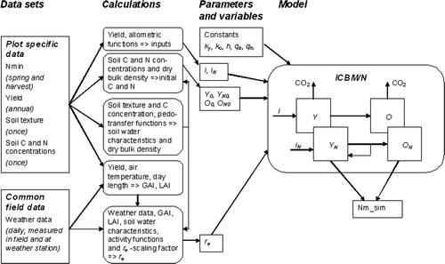
ICBM/N model

The ICBM family of analytically solved soil carbon and nitrogen models is described in detail by Andrén and Kätterer (1997) and Kätterer and Andrén (2001) and only a brief description of the coupled C/N model used (ICBM/N) will be given here (see http://www-mv.slu.se/vaxtnaring/olle/forprogramsinExcelandSAS).

Two C and two organic N pools are defined (Figure 1, inside box); young and old carbon (Y and O) and young and old nitrogen (Y _N and O _N ). C and N in crop residues (i, i/q _i ) are input to Y and Y _N , respectively. During decomposition, C will be lost either as carbon dioxide or enter the O pool according to the value of the humification coefficient (h), while N will be mineralized or immobilized according to the Y/Y _N ratio, the C/N ratio of the organism community (q _b ) and its yield efficiency (e _y ). The amount of N entering O _N is determined by the C/N ratio O/O _N (q _h ). Outflows from the pools follow first-order kinetics and the rate constants k _y and k _o are modified by a factor (r _e ), into which all external effects (soil moisture and temperature in our application) are condensed (Andrén & Kätterer, 1997). Initial states and parameter values are presented in Table II.

Table II. Initial conditions, driving variables and parameter values, symbols and units used in this application of the ICBM/N model.

Model input	Symbol	Unit	Notes	References^a
Initial conditions
Initial total C mass	C 0	kg ha^−1	Average 52 104, min 41 827, max 62 080	1
Initial C mass of the ‘young ’ pool	Y 0	kg ha^−1	Average 6000, min 5025, max 6731	2
Initial C mass of the ‘old’ pool	O 0	kg ha^−1	= C 0 –Y 0 , Average 46 104, min 36 280, max 56 008	1
Initial total N mass in soil organic matter	N 0	kg ha^−1	Average 4014, Min 2988, Max 5211	1
Initial N mass of the 'young’ pool	Y N0	kg ha^−1	Y N0 = Y 0 /q Y0 . Average 192, min 157, max 219	2
Initial N mass of the 'old’ pool	O N0	kg ha^−1	O N0 = N 0 –Y N0 . Average 3822, min 2814, max 5041	1
Driving variables
Annual C input to soil	i	kg year^−1	Inputs for harvest year 1998 are included in Y 0	1
			1999: Average 4435, min 3664, max 5107
			2000: Average 3053, min 2328, max 3634
Quality, C/N ratio of Y0	q Y0		Average 31
Quality, C/N ratio of input, i	q i	–	Inputs for harvest year 1998 are included in Y N0	1
			1999: Average 53.7
			2000: Average 53.7
Climate response	r e	–	See Materials and methods
Fixed parameters
Decomposition rate constant for young pool	k y	year^−1	0.8	3
Decomposition rate ‘constant’ for the old pool	k o	year^−1	0.006	3
Humification coefficient, fraction of ‘young’ outflux to O	h	–	0.125	3
C/N ratio of soil organism biomass	q b	–	5	4
C/N ratio of the ‘humification’, the influx to O	q h	–	10	4
Optimized parameters
External response factor that affects out flux from ‘young’ and ‘old’	k r	–	10.5	5
Water filled porosity at maximum mineralization rate	γ	–	0.5 (bounds: 0.5< γ <1)	5
Efficiency, the fraction of C flux from Y allocated to organism growth	e y	–	0.211 (bounds: 0.2< e y <0.3)	5
^a(1) derived from measurements; (2) from previous experience; (3) Andrén and Kätterer (1997); (4) Kätterer and Andrén (2001); (5) estimated by non-linear regression analysis (see Materials and methods).

Calculating the external response (re)

A daily decomposer activity factor, r _e , is calculated from soil water content (θ; m³ m⁻³) and soil temperature (T; °C). This factor is the product of the daily outputs of the response functions r _T and r _θ , depending on θ and T, respectively. T is assumed to affect decomposer activity according to a quadratic relationship (Ratkowsky et al., 1982), which was normalized for 30 °C, roughly the maximum soil temperature occurring at the site:

1

where activity is zero at T _min = − 3.8 °C (Kätterer et al., 1998).

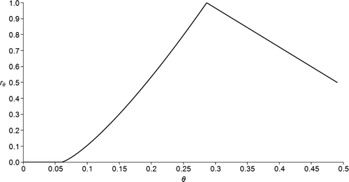
The moisture response function (r _θ ) was assumed to depend on θ in the following way:

2

where microbial activity increases from zero at a certain fraction (α; here set to 0.5) of the water content at wilting point (θ _wp ) to a maximum at the optimal water content (γθ _s ), corresponding to a fraction γ of the saturated water content (θ _s ). Above γθ _s , r _θ decreases again to a minimum of r _s at θ _s . The parameter β (=1.3) defines the shape of the function between αθ _wp and γθ _s (Figure 2). This water response function is similar to those implemented in other decomposition and ecosystem models like NLEAP (Schaffer et al., 2001), and is based on the experimental work by Linn and Doran (1984) and Lomander et al. (1998). The values for θ _wp and θ _s were estimated from soil texture and carbon concentrations using pedotransfer functions (Kätterer et al., 2006).

Figure 2.  Example of relation between θ (soil water content) and the value of r _θ (moisture response function) according to eq. (2). θwp =0.12, θfc =0.35 and ε =0.49.

The product r _T r _θ gives only relative response values since the default decomposition rate constants, k _Y and k _O , in the model refer to annual mean r _e -values, which are normally close to unity in the climate conditions of central Sweden (i.e. in the Uppsala region; Andrén & Kätterer, 1997). Thus, r _T r _θ must be scaled so that the sum of all daily products over the year corresponds to r _e in ICBM:

3

where the scaling factor, k _r , was used as a free scaling parameter in the calculations (see below).

The resulting daily r _e -values (r _{e_day} ) were summed over the experimental period. When applying the ICBM model to the data, in analogy with the use of temperature sums, we replaced time (t) as the independent variable by r _e , the ‘climate sum’:

4

Thus, we did not have to run simulations, since the model is analytically solved and both t and r _e are quasi-continuous variables. Instead, solutions could be found using non-linear regression (Kätterer & Andrén, 2001).

Soil temperature and moisture data are needed for calculating r _e (according to Eqs 1 and 2). For the periods outside the growing season soil temperature was not measured, but instead estimated from air temperature and leaf area using an empirical model driven by air temperature and leaf area index (Bolinder et al., 2008; Kätterer & Andrén, 2008). Simple soil water balance calculations based on FAO concepts (Allen et al., 1998) were used to calculate daily soil water content for each plot within the field. Inputs are daily weather station data (daily mean air temperature, precipitation and reference evapotranspiration), soil water characteristics and green area index of the crop. The soil characteristics needed for running this model for a certain soil (i.e. water content at wilting point, θ _wp and field capacity, θ _fc ) were estimated from soil texture and carbon concentrations using the pedotransfer functions proposed by Kätterer et al. (2006). Green area index, GAI, here defined as the area of all plant parts that are visibly green (only one side of leaves is counted) represents the influence of the crop on the soil water balance. GAI dynamics over the growing season were described by a bell-shaped function (Bolinder et al., 2008):

5

where t is day of year, µ is the day at which GAI=GAI _max (maximum GAI) and σ determines the crop-specific width of this distribution function. Values for σ were estimated from Swedish data sets for winter wheat and spring barley (Flink et al., 1995). An empirical relationship between the amplitude of this function (GAI _max ) and grain yield (Mg ha⁻¹ dry matter) was calculated using experimental results for barley and winter wheat (n = 28) compiled from Swedish and Danish field experiments (Pettersson, 1989; Flink et al., 1995; Olesen et al., 2002). For the Danish data set, a harvest index of 0.4 was assumed for winter wheat. The resulting regression equation (GAI _max =0.073*Yield ² +0.408*Yield) explained 89% of the variation in GAI _max . Accordingly, GAI _max was calculated from grain yield records for each year in the 34 plots.

The scaling of this function in time from the date of sowing, which was known, to emergence and anthesis (where GAI was assumed to be maximum) was performed using empirical functions for phenological development of the canopy, which were driven by air temperature sums and day length (T _sd ) according to Pettersson (1989) and Olesen et al. (2002).

Model application

Three model parameters were optimized simultaneously for all 34 locations within the field by minimizing the deviations between apparent Nm and calculated Nm_sim. The optimized parameters were the scaling factor for the decomposition rates (k _r ), which only scales the rate and does not affect differences between plots, the proportion of water-filled pore space when r _θ is optimum (γ) and the efficiency of soil microorganisms in converting C into biomass (e _y ). All other parameter values were either taken from previous publications, based on measurements, or estimated from pedotransfer functions (Table II).

The inputs of C and N (i and i/q _i , respectively) to the soil were assumed to occur once a year, at ploughing in the autumn. No straw was removed from the field during the experiment. The amounts of straw, other above-ground residues and roots including root turnover and root exudates were calculated from grain yield data using allometric relationships (Andrén et al., 2004). The amount of N in straw and other crop residues was assumed to be 8.2 mg g⁻¹ dry matter and for the below-ground C input we assumed a C/N ratio of 50 (Andrén et al., 1990). All parameter values are listed in Table II.

For 1998, the model was executed only to allow the model pools to adjust to known inputs and conditions, and Nm values from 1998 were not used for the optimization. Y and Y _N were initialized assuming quasi steady-state conditions. On 1 January 1998, an average C or N mass of 6.0 and 0.19 Mg ha⁻¹ in Y and Y _N , respectively, which approximately correspond to the average steady-state values of these pools over the field, was distributed between the 34 grid points according to the relative differences between the simulated pool sizes on 1 January 1999, 2000 and 2001.

Statistical analyses

The model was run using SAS software (SAS Inst. Inc., 2004). Model parameters were optimized using a modified Gauss–Newton method (non-linear regression analysis, Proc NLIN; SAS Institute Inc., 2004). Bounds for parameter values are presented in Table II. To avoid local minima in the optimization function, the model was initialized with several different combinations of parameter values within these bounds. All runs resulted in the same parameter estimate (Table II). We also used stepwise linear regression for evaluating the relationship between different explanatory variables and apparent net N mineralization. The adjusted coefficient of determination () was used as a criterion of model fit (Minitab Inc, 2007).

Results

Apparent net N mineralization (Nm) regressed on different explanatory variables

We tested the ability of nine potential predictor variables (growing season, i, i/q _i , C ₀ , N ₀ , Y _N0 , clay, silt, and sand) to explain Nm (Table III). In a stepwise linear regression analysis, the variable growing season explained 43% of the variation in Nm between plots during the two seasons. The initial amount of total soil N (N ₀ ) explained an additional 14% and silt and i/q _i explained another 4 and 2%, respectively. Taken together, these four variables explained 62% of the total variation. When applying the regression model on each growing season separately, a considerably smaller proportion of total variation was explained for 1999 (22%) and an intermediate proportion (42%) in 2000.

Table III. Cumulative -values according to stepwise linear regression analysis starting with nine variables (growing season, C ₀ , N ₀ , Y _N0 , i, i/q _i , clay, sand, silt) potentially explaining the variation in apparent net N mineralization. The critical p-value for variable exclusion was 0.15. NA = not applicable.

	1999	2000	1999–2000
Explanatory variable	n = 34	n = 33	n = 67
Growing season	NA	NA	0.43
Growing season, N 0	0.14	0.34	0.57
Growing season, N 0, Silt	0.22	0.37	0.60
Growing season, N 0, Silt, i/q i	–	0.42	0.62

Calculation of soil water characteristics

Despite relatively large differences in soil texture between the plots, the differences in θ _wp and θ _fc between clayey and sandy plots as estimated with the pedotransfer functions were relatively small and the difference in resulting plant available water storage capacity (θ _fc −θ _wp ) was even smaller (Table IV). In clayey plots, water storage capacity was 0.28–0.32 and in sandy plots 0.25–0.34 m³ m⁻³. Consequently, soil water dynamics were similar in all plots (Figure 3). This graph also reflects the fact that precipitation was relatively high during the growing seasons of 1999 and 2000. Soil water content never came close to θ _wp . On some days, soil water content was higher than θ _fc , which is a consequence of the design of the water balance model, in which water above θ _fc is drained the day after the precipitation event.

Figure 3.  Dynamics of soil water content (θ; m³ m⁻³) in 0–0.2 m depth in one ‘sandy’ plot (a) and in a clayey plot (b). The dotted lines show θ _fc and θ _wp .

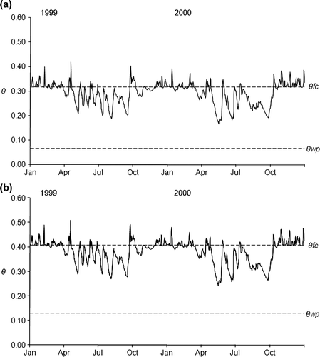
Table IV. Mean, minimum and maximum values and standard deviations (σ) of physical soil properties in the clayey and sandy areas within the experimental field. Wilting point, field capacity, plant available water capacity, porosity and dry bulk density calculated from pedotransfer functions (Kätterer et al. 2006).

	Symbol	Mean	Min	Max	σ
Clayey plots
Silt		0.524	0.451	0.577	0.001
Wilting point	θ wp	0.117	0.0988	0.130	0.00724
Field capacity	θ fc	0.422	0.401	0.438	0.0109
Plant available water capacity	θ fc – θ wp	0.305	0.277	0.318	0.0115
Porosity	ε	0.515	0.493	0.529	0.0111
Dry bulk density, Mg m^−3	ρ	1.28	1.25	1.33	0.0242
Sandy plots
Silt		0.275	0.193	0.412	0.003
Wilting point	θ wp	0.0764	0.0628	0.087	0.00714
Field capacity	θ fc	0.369	0.317	0.426	0.0295
Plant available water capacity	θ fc – θ wp	0.293	0.250	0.345	0.235
Porosity	ε	0.514	0.480	0.554	0.0204
Dry bulk density, Mg m^−3	ρ	1.27	1.17	1.36	0.0539

Optimized parameters

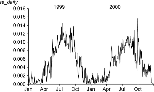
The optimized values of the three free parameters are presented in Table II. The value for γ (fraction of water-filled porosity at maximum heterotrophic soil activity) was 0.5, which was the lower boundary set in the optimization procedure, and which corresponds to γθ _s values of between 0.24 and 0.28 m³ m⁻³ in the plots. The estimated value for k _r (10.5) implies that annual r _e was 1.72 for 1999 and 1.73 for 2000 and r _e during the growing seasons of 1999 and 2000 was 1.05 and 1.13, respectively.

The temporal dynamics of r _e during the two years are exemplified for one plot (Figure 4). The optimized value for e _y (microbial growth efficiency) was 0.21 and was only moderately correlated with k _r (r = − 0.23). No correlation was calculated for γ since it reached the lower allowed limit of the parameter interval.

Figure 4.  Daily values of the climate response variable, r _e , in one ‘sandy’ plot during 1999 and 2000.

Net N mineralization

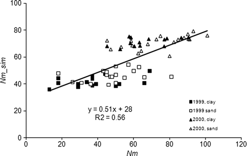
The estimated mean Nm_sim values matched the measured mean Nm values exactly, which were 44 and 71 kg N ha⁻¹ during the growing seasons 1999 and 2000, respectively. However, the model underestimated the variation in Nm among the 34 grid points. Corresponding standard deviations of the estimated mean values were 7.1 and 5.4 and those for the measurements were 15 and 16 kg N ha⁻¹ in 1999 and 2000, respectively. For both years together, the model explained 56% of the total variation (Figure 5). The largest deviation from measured Nm was 34 kg ha⁻¹. The standard deviation of the difference between Nm_sim and Nm was 13.8 kg ha⁻¹, while approximately half of the estimated values deviated by less than 10 kg ha⁻¹ from the mean. For the years 1999 and 2000 separately, the standard deviation of the differences were 14.8 and 13.5 kg for the estimated and 34 and 30 for the measurements, respectively, and the model explained 20% and 27% of the variation.

Figure 5.  Relationship between measured (Nm) and estimated apparent net N mineralization (Nm_sim) during 1999 and 2000.

Regression including r_e

The estimated climate factor r _e accounted for the mean differences in Nm between the two growing seasons. r _e was the first variable to be included in the stepwise multiple linear regressions described above, and it explained 36% of the variation. Thereafter, only N ₀ (2%) was significant. For single growing seasons, N ₀ was the most significant variable. In 1999, N ₀ explained 14% of the variation and silt explained another 8%. In 2000, N ₀ explained 34% of the variation and r _e explained 8%.

Discussion

The observed Nm values during 1999 were similar to previous measurements in this area, whereas those for 2000 were generally higher (Lindén et al., 1992). According to a previous study, partly using the same data set (Delin & Lindén, 2002), within-field variation in Nm was moderately but significantly positive correlated with total soil C and N concentrations during three years (correlation coefficients between 0.34 and 0.49). Correlations between Nm and clay content were not consistent between years: Nm at a certain location could be relatively large during one year compared with the field mean and relatively small during the other years at the same location.

According to the regression on input variables in this study, total N in soil organic matter N ₀ was the second most important variable after growing season over the two seasons, and the most significant within each year. It is not surprising that the amount of N potentially available for mineralization is crucial for determining how much N is mineralized. N ₀ accounted for 67–75% of the fraction of the within-seasonal variation in Nm that was explained by the regression model. The next most important variable for explaining the variation in Nm was i/q _i (N input into soil), which had some significance during the two seasons 1999 – 2000 and for the single season 2000 (Table III). The positive sign of the regression coefficient indicates that N added in plant residues may have contributed to net mineralization during the year after incorporation and not to net immobilization of N, as could be expected from their high C/N ratio. Silt was the third factor included in the regression model for 1999–2000. According to Kätterer et al. (2006), the plant available water storage capacity is highly correlated with silt in Swedish soils and it is probable that N mineralization was higher at locations with higher water storage capacities, as shown by others (e.g. Smithwick et al., 2005).

In the regression model, the effect of growing season could to a great extent be substituted by r _e which indicates that the climate factor could account for the major differences in Nm between the two growing seasons. The dynamic model accounted for 56% of the variation in Nm during the two years, but a smaller proportion of the within-year variation in Nm could be explained. In the context of using this approach in practical applications, to adjust fertilizer doses to within-field variation in soil properties, predictive power has to be improved. The moderate precision is probably due to both model assumptions and limitations of the measurements as discussed below.

Model limitations

The description of carbon and nitrogen turnover in our model is similar to those implemented in many other soil C and N models. ICBM/N has earlier been applied to data series at different time scales and proved to give valid results (Kätterer & Andrén, 2001). Three parameters were optimized in the simulation. The optimized k _r -value (normalization constant) resulted in values for r _e within the range of values observed in earlier Swedish applications with the ICBM model (Kätterer & Andrén, 1999; Kätterer et al., 2004; Andrén et al., 2007; Bolinder et al., 2007; Kätterer et al., 2008). The optimized value for e _y (microbial growth efficiency) was within reasonable limits (Kätterer & Andrén, 2001). During the optimization of γ, the lower allowed limit in the fitting procedure (0.5) was reached. This means that biological activity in the model was highest when 50% of the soil pores were filled with water and that N mineralization rates decreased between 50 and 100% water-filled pores (according to eq. 2). This may indicate N losses at high water content such as denitrification and N leaching, as also discussed by Delin et al. (2005). The variation in simulated apparent net N mineralization (Nm_sim) was smaller than that in the measurements, something that has also been noted in other modelling exercises (Kersebaum et al., 2005). Besides r _e , initial total N as well as C and N inputs from previous years were site-specific variables. Since these were only moderately correlated with Nm, the variation in Nm_sim should have been mainly generated by the variation in r _e . However, the variation in r _e was much smaller than that of Nm. The fact that we did not have high-resolution site-specific information on soil temperature may be one possible reason for this. The assumptions behind the water balance model and the estimation of dry bulk density set other limitations, which are further discussed below. We tested different temperature response functions (Kätterer et al., 1998), but these affected the model outcome only marginally. The simulated soil water content at the different locations was probably more critical for the model outcome. However, the calculated variation in plant available water between locations was small, which is in accordance with measurements at other locations in the same field (Delin et al., 2005).

How to account for the effects of soil water content on biological activity is still actively discussed in the literature (e.g. Schjønning et al., 2003; Thomsen et al., 2003; Cook & Orchard, 2008) and water response functions vary considerably between different decomposition and ecosystem models (e.g. Rodrigo et al., 1997). The approach used here should be reasonably valid since the critical parameter was free to vary within certain limits in the simulations. The uncertainty introduced by the estimation of the two key parameters in the water balance model, θ _fc and θ _wp , is probably more problematic. Although the overall performance of the pedotransfer functions used to estimate these parameters is quite good, the accuracy for the prediction of individual values is low (Kätterer et al., 2006). The same applies to the estimates of dry bulk density. The other components of the water balance such as precipitation and evapotranspiration were probably also sources of error which will interact with horizontal and vertical soil water flows due to topographic position, capillarity, distance to drainage pipes and ground water level. However, the spatially explicit calculation of these processes is sometimes ambiguous even when using complex water and heat models (Schmidt & Persson, 2003; Reuter et al., 2005; Bechtold et al., 2007) and the use of two- or three-dimensional complex models is not realistic for practical applications.

Measurements

The uptake of N from below 0.2 m depth was not considered in the calculation of Nm_sim. Although uptake from deeper layers can be considered as a minor part of crop N uptake (Johansson, 1992), it will result in an overestimation of Nm_sim if not counteracted by a corresponding downward transport of mineral N during the growing seasons. However, within-field variation in Nm_sim will not be affected if this error is similar between field locations and does not change with time. N in roots is not included in the estimates, which again should not significantly affect the relative difference between field locations. Nevertheless, differences in rooting pattern and N uptake from different depths between spring barley (1999) and winter wheat (2000) may have introduced some bias in Nm_sim.

Considerable small-scale spatial variation of soil and crop variables due to landscape heterogeneity is often observed (Lindén, 1981; Strong et al., 1998; Giebel et al., 2006). In an agricultural field in Germany, 35–49% of the total spatial variation in mineral N originated from small-scale variability observed at distances of < 5 m and from sampling and analytical errors (Giebel et al., 2006). No spatial structure in mineral N may be found in highly heterogeneous forest soils (Smithwick et al., 2005, Garten et al., 2007) but in more homogeneous landscapes, autocorrelations within a distance of 40 m have been found in an agricultural soil (Van Meirvenne et al., 2003).

In a Swedish field experiment with winter wheat, Kätterer and Andrén (1996) found that variation in above-ground crop N at harvest was almost as large within experimental units as between them. The average standard deviations were 16 and 19 kg N ha⁻¹, respectively. In our experiment, changes in mineral N between spring and autumn were much smaller than the amount of N found in the above-ground crop, and thus the variation in Nm mainly depended on differences in the estimates of crop N uptake.

Thus, small-scale variation means that a correct sampling strategy is of the utmost importance. Sampling should be done with a suitable number of sub-samples and it is equally vital that the samples refer to the same spatial scale (Western & Blöschl, 1999). In this experiment, texture and SOC concentrations were sampled for each plot at the initiation of the experiment and mineral N and crop was sampled in subplots every year. This was necessary, since the experimental plots were moved slightly from year to year to an untreated position that was fertilized in the same way as the field as a whole according to prevailing farming practices. Between two adjacent plots, 50 m apart, SOC amounts varied from 52 to 69 Mg ha⁻¹. However, the variability of SOC inside plots is unknown. In a study on arable fields in south eastern Norway, Kværnø et al. (2007) estimated the variogram range for carbon concentrations to be about 40 m. In grassland, SOC storages varied by a factor two within fields and a high nugget/sill ratio indicating a high degree of small-scale variation (Don et al., 2007). Similar results were presented by Mestdagh et al. (2006). Therefore, variation in SOC storage is probably a main source of error in the calculations, and this constitutes a major hurdle for testing the validity of soil carbon models and hypotheses (Andrén et al., 2008). A perfect match between model and observations cannot be expected due to the high variation in observations at small scales and uncertainty in input data. Every effort should be made to reduce these errors and uncertainties (Kersebaum et al., 2005; Foereid et al., 2007; Pedersen et al., 2007).

In the experiment, N mineralization was estimated as Nm=N _c +ΔNmin. This implies the assumption that no N other than that taken up by the crop is lost from the topsoil. However, during the experimental period heavy rains resulted in water surplus at several occasions. This could have led to redistribution of water within the field due to surface runoff and consequently to losses of N through both denitrification and leaching, predominantly at the wettest locations within the field. Modelling the distribution of rainfall and redistribution of water in the field due to topography and variation in water conductivity is generally a complex task (Schmidt & Persson, 2003) and outside the scope of this paper. Nevertheless, we simulated ponding water within the field using a simple water balance model. However, this did not result in any significant correlation between simulated excess water and the deviation between Nm and Nm_sim within the growing seasons (data not shown). Even if a model accurately could estimate amounts of N mineralized at each location within a field, it would be of limited practical value if the N losses are large compared with N mineralization. In these cases, a model predicting losses is more useful than a mineralization model. Although ICBM/N was able to represent variation in net N mineralization between growing seasons the full spatial variation could not be matched. Nevertheless, we believe that it is extremely important to publish results not giving significant correlations, since only selecting ‘successful’ model exercises gives a biased view of the actual problems remaining (Andrén et al., 2008).

N mineralization models have proven to be useful for illustrating principles, the main variables involved, and significant mass flows in the mineralization process. Nevertheless, with present techniques used in practical farming, it is difficult to measure the key variables in a field with adequate precision for accurate modelling of N mineralization at medium to high resolution in space in time. Considerable improvements to the current methodology as well as new approaches are necessary.

Acknowledgements

Financial support was provided from the Swedish Farmer's Foundation for Agricultural Research

References

- Allen , R. G. , Pereira , L. S. , Raes , D. and Smith , M. 1998 . Crop evapotranspiration. Guidelines for computing crop water requirements , Rome : FAO .
- Andrén , O. and Kätterer , T. 1997 . ICBM: The Introductory Carbon Balance Model for exploration of soil carbon balances . Ecological Applications , 7 : 1226 – 1236 .
- Andrén , O. and Kätterer , T. 2001 . “ Basic principles for soil carbon sequestration and calculating dynamic country-level balances including future scenarios ” . In Assessment methods for soil carbon , Edited by: Lal , R. , Kimble , J. M. and Follett , R. F. 495 – 511 . New York : Lewis Publishers .
- Andrén , O. , Kihara , J. , Bationo , A. , Vanlauwe , B. and Kätterer , T. 2007 . Soil climate and decomposer activity in sub-Saharan Africa estimated from standard weather station data: A simple climate index for soil carbon balance calculations . AMBIO: A Journal of the Human Environment , 36 : 379 – 386 .
- Andrén , O. , Kätterer , T. and Karlsson , T. 2004 . ICBM regional model for estimations of dynamics of agricultural soil carbon pools . Nutrient Cycling in Agroecosystems , 70 : 231 – 239 .
- Andrén , O. , Kirchmann , H. , Kätterer , T. , Magid , J. , Paul , E. A. and Coleman , D. C. 2008 . Visions of a more precise soil biology . European Journal of Soil Science , 59 : 380 – 390 .
- Andrén , O. , Lindberg , T. , Boström , U. , Clarholm , M. , Hansson , A.-C. , Johansson , G. , Lagerlöf , J. , Paustian , K. , Persson , J. , Pettersson , R. , Schnürer , B. , Sohlenius , B. and Wivstad , M. 1990 . “ Organic carbon and nitrogen flows ” . In Ecological Bulletines , Edited by: Andrén , O. , Lindberg , T. , Paustian , K. and Rosswall , T. Vol. 40 , 85 – 126 . Copenhagen : Munksgaard International Booksellers .
- Bechtold , I. , Kohne , S. , Youssef , M. A. , Lennartz , B. and Skaggs , R. W. 2007 . Simulating nitrogen leaching and turnover in a subsurface-drained grassland receiving animal manure in Northern Germany using DRAINMOD-N II . Agricultural Water Management , 93 : 30 – 44 .
- Biermacher , J. T. , Epplin , F. M. , Brorsen , B. W. , Solie , J. B. and Raum , W. R. 2006 . Maximum benefit of a precise nitrogen application system for wheat . Precision Agriculture , 7 : 193 – 204 .
- Bolinder , M. A. , Andren , O. , Kätterer , T. , de Jong , R. , VandenBygaart , A. J. , Angers , D. A. , Parent , L. E. and Gregorich , E. G. 2007 . Soil carbon dynamics in Canadian Agricultural Ecoregions: Quantifying climatic influence on soil biological activity . Agriculture, Ecosystems & Environment , 122 : 461 – 470 .
- Bolinder , M. A. , Andren , O. , Kätterer , T. and Parent , L.-E. 2008 . Soil organic carbon sequestration potential for Canadian Agricultural Ecoregions calculated using ICBMregion . Canadian Journal of Soil Science , 88 : 1 – 10 .
- Börjesson , T. , Stenberg , B. , Linden , B. and Jonsson , A. 1999 . NIR spectroscopy, mineral nitrogen analysis and soil incubations for the prediction of crop uptake of nitrogen during the growing season . Plant and Soil , 214 : 75 – 83 .
- Cook , F. J. and Orchard , V. A. 2008 . Relationships between soil respiration and soil moisture . Soil Biology and Biochemistry , 40 : 1013 – 1018 .
- Delin , S. and Berglund , K. 2005 . Management zones classified with respect to drought and waterlogging . Precision Agriculture , 6 : 321 – 340 .
- Delin , S. and Lindén , B. 2002 . Relations between net nitrogen mineralization and soil characteristics within an arable field . Acta Agriculturae Scandinavica. Section B, Soil and Plant Science , 52 : 78 – 85 .
- Delin , S. , Linden , B. and Berglund , K. 2005 . Yield and protein response to fertilizer nitrogen in different parts of a cereal field: Potential of site-specific fertilization . European Journal of Agronomy , 22 : 325 – 336 .
- Delin , S. and Söderström , M. 2002 . Performance of soil electrical conductivity and different methods for mapping soil data from a small data set . Acta Agriculturae Scandinavica. Section B, Soil and Plant Science , 52 : 127 – 135 .
- Don , A. , Schumacher , J. , Scherer-Lorenzen , M. , Scholten , T. and Schulze , E.-D. 2007 . Spatial and vertical variation of soil carbon at two grassland sites – Implications for measuring soil carbon stocks . Geoderma , 141 : 272 – 282 .
- Flink , M. , Pettersson , R. and Andrén , O. 1995 . Growth dynamics of winter wheat in the field with daily fertilization and irrigation . Journal of Agronomy and Crop Science , 174 : 239 – 252 .
- Foereid , B. , Barthram , G. T. and Marriot , C. A. 2007 . The CENTURY model failed to simulate soil organic matter development in an acidic grassland . Nutrient Cycling in Agroecosystems , 78 : 143 – 153 .
- Garten , C. T. Jr , Kang , S. , Brice , D. J. , Schadt , C. W. and Zhou , J. 2007 . Variability in soil properties at different spatial scales (1 m–1 km) in a deciduous forest ecosystem . Soil Biology and Biochemistry , 39 : 2621 – 2627 .
- Giebel , A. , Wendroth , O. , Reuter , H. I. , Kersebaum , K. C. and Schwarz , J. 2006 . How representatively can we sample soil mineral nitrogen? . Journal of Plant Nutrition and Soil Science , 169 : 52 – 59 .
- Godwin , R. J. , Wood , G. A. , Taylor , J. C. , Knight , S. M. and Welsh , J. P. 2003 . Precision farming of cereal crops: a review of a six year experiment to develop management guidelines . Biosystems Engineering , 84 : 375 – 391 .
- Joernsgaard , B. and Halmoe , S. 2003 . Intra-field yield variation over crops and years . European Journal of Agronomy , 19 : 23 – 33 .
- Johansson , G. 1992 . Below-ground carbon distribution in barley (Hordeum vulgare L.) with and without nitrogen fertilization . Plant and Soil , 144 : 93 – 99 .
- Karlsson , T. , Andrén , O. , Kätterer , T. and Mattsson , L. 2003 . Management effects on topsoil carbon and nitrogen in Swedish long-term field experiments – budget calculations with and without humus pool dynamics . European Journal of Agronomy , 20 : 137 – 147 .
- Kätterer , T. , Andersson , L. , Andrén , O. and Persson , J. 2008 . Long-term impact of chronosequential land use change on soil carbon stocks on a Swedish farm . Nutrient Cycling in Agroecosystems , 81 : 145 – 155 .
- Kätterer , T. and Andrén , O. 1996 . Measured and simulated nitrogen dynamics in winter wheat and a clay soil subjected to drought stress or daily irrigation and fertilization . Fertilizer Research , 44 : 51 – 63 .
- Kätterer , T. and Andrén , O. 1999 . Long term agricultural field experiments in Northern Europe: Analysis of the influence of management on soil carbon stocks using the ICBM model . Agriculture, Ecosystems and Environment , 72 : 165 – 179 .
- Kätterer , T. and Andrén , O. 2001 . The ICBM family of analytically solved models of soil carbon, nitrogen and microbial biomass dynamics – descriptions and application examples . Ecological Modelling , 136 : 197 – 207 .
- Kätterer , T. & Andrén , O. 2008 Predicting daily soil temperature profiles in arable soils in cold temperate regions from air temperature and leaf area index . Acta Agriculturae Scandinavica. Section B, Soil and Plant Science , doi: DOI: 10.1080/09064710801920321 .
- Kätterer , T. , Andrén , O. and Jansson , P. E. 2006 . Pedotransfer functions for estimating plant available water and bulk density in Swedish agricultural soils . Acta Agriculturae Scandinavica. Section B, Soil and Plant Science , 56 : 263 – 276 .
- Kätterer , T. , Andrén , O. and Persson , J. 2004 . The impact of altered management on long-term agricultural soil carbon stocks – a Swedish case study . Nutrient Cycling in Agroecosystems , 70 : 179 – 187 .
- Kätterer , T. , Reichstein , M. , Andrén , O. and Lomander , A. 1998 . Temperature dependence of organic matter decomposition: A critical review using literature data analyzed with different models . Biology and Fertility of Soils , 27 : 258 – 262 .
- Kersebaum , K. C. , Lorenz , K. , Reuter , H. I. , Schwarz , J. , Wegehenkel , M. and Wendroth , O. 2005 . Operational use of agro-meteorological data and GIS to derive site specific nitrogen fertilizer recommendations based on the simulation of soil and crop growth processes . Physics and Chemistry of the Earth, Parts A/B/C , 30 : 59 – 67 .
- Kværnø , S. H. , Haugen , L. E. and Børresen , T. 2007 . Variability in topsoil texture and carbon content within soil map units and its implications in predicting soil water content for optimum workability . Soil and Tillage Research , 95 : 332 – 347 .
- Lindén , B. 1981 . Ammonium- och nitratkvävets rörelser och fördelning i marken. II Metoder för mineralkväveprovtagning och analys (Movement and distribution of ammonium- and nitrate-N in the soil. II Methods of sampling and analysing mineral nitrogen) . Swedish University of Agricultural Sciences, Dept. of Soil Sciences, Division of Soil Fertility , Rep. No. 137 , Uppsala (in Swedish)
- Lindén , B. , Lyngstad , I. , Sippola , J. , Søegard , K. and Kjellerup , V. 1992 . Nitrogen mineralization during the growing season I. Contribution to the nitrogen supply of spring barley . Swedish Journal of Agricultural Research , 22 : 3 – 12 .
- Linn , D. M. and Doran , J. W. 1984 . Effect of water-filled pore space on carbon dioxide and nitrous oxide production in tilled and no-tilled soils . Soil Science Society of America Journal , 48 : 1267 – 1272 .
- Lomander , A. , Kätterer , T. and Andrén , O. 1998 . Modelling the effects of temperature and moisture on CO2 evolution from top- and subsoil using multi-compartment approach . Soil Biology and Biochemistry , 30 : 2023 – 2030 .
- Mestdagh , I. , Lootens , P. , Cleemput , O. V. and Carlier , L. 2006 . Variation in organic-carbon concentrations and bulk density in Flemish grassland soils . Journal of Plant Nutrition and Soil Science , 169 : 616 – 622 .
- Minitab Inc. Minitab 15 2007 . Minitab Inc .
- Olesen , J. E. , Petersen , B. M. , Berntsen , J. , Hansen , S. , Jamieson , P. D. and Thomsen , A. G. 2002 . Comparisons of methods for simulating effects of nitrogen on green area index and dry matter growth in winter wheat . Field Crops Research , 74 : 131 – 149 .
- Pedersen , A. , Petersen , B. M. , Eriksen , J. , Hansen , S. and Jensen , L. S. 2007 . A model simulation analysis of soil nitrate concentrations – Does soil organic matter pool structure or catch crop growth parameters matter most? . Ecological Modelling , 205 : 209 – 220 .
- Pettersson , R. 1989 . Above-ground growth dynamics and net production of spring barley in relation to nitrogen fertilization . Swedish Journal of Agricultural Research , 19 : 135 – 145 .
- Ratkowsky , D. A. , Olley , J. , McMeekin , T. and Ball , A. 1982 . Relationship between temperature and growth rate of bacterial cultures . Journal of Bacteriology , 149 : 1 – 5 .
- Reusch , S. 1997 . Entwiklung eines reflexionsoptischen sensors zur erfassung der stickstoffversorgung landwirtschaftlicher kulturpflanzen . Dissertation, Kiel .
- Reuter , H. , Giebel , A. and Wendroth , O. 2005 . Can landform stratification improve our understanding of crop yield variability? . Precision Agriculture , 6 : 521 – 537 .
- Rodrigo , A. , Recous , S. , Neel , C. and Mary , B. 1997 . Modelling temperature and moisture effects on C-N transformations in soils: Comparison of nine models . Ecological Modelling , 102 : 325 – 339 .
- SAS Institute Inc . 2004 . SAS 9.1.3 help and documentation . Cary, NC : SAS Institute Inc .
- Schaffer , M. , Lasnik K , O X. & Flynn , R. 2001 . NLEAP internet tools for estimating NO3-N leaching and N2O emissions . In M. Schaffer , L. Ma , and S. Hansen Modeling carbon and nitrogen dynamics for soil management , pp. 403 426 . Boca Raton, FL : CRC Press .
- Schjønning , P. , Thomsen , I. K. , Moldrup , P. and Christensen , B. T. 2003 . Linking soil microbial activity to water- and air-phase contents and diffusivities . Soil Science Society of America Journal , 67 : 156 – 165 .
- Schmidt , F. and Persson , A. 2003 . Comparison of DEM data capture and topographic wetness indices . Precision Agriculture , 4 : 179 – 192 .
- Smithwick , E. A. H. , Mack , M. C. , Turner , M. G. , Chapin , F. S. I. , Zhu , J. and Balser , T. C. 2005 . Spatial heterogeneity and soil nitrogen dynamics in a burned black spruce forest stand: Distinct controls at different scales . Biogeochemistry , 76 : 517 – 537 .
- Stenberg , B. , Börjesson , T. & Jonsson , A. 2002 . Near infrared reflectance spectroscopy – a rapid method for predictive field mapping of soil-N mineralization? DIAS Report 84, Plant Production .
- Strong , D. T. , Sale , P. W. G. and Helyar , K. R. 1998 . The influence of the soil matrix on nitrogen mineralization and nitrification. I. Spatial variation and a hierarchy of soil properties . Australian Journal of Soil Research , 36 : 429 – 447 .
- Thomsen , I. K. , Schønning , P. , Olesen , J. E. and Christensen , B. T. 2003 . C and N turnover in structurally intact soils of different texture . Soil Biology and Biochemistry , 35 : 765 – 774 .
- Van Meirvenne , M. , Maes , K. and Hofman , G. 2003 . Three-dimensional variability of soil nitrate-nitrogen in an agricultural field . Biology and Fertility of Soils , 37 : 147 – 153 .
- Western , A. W. and Blöschl , G. 1999 . On the spatial scaling of soil moisture . Journal of Hydrology , 217 : 203 – 224 .