Exploring structural sediment connectivity via surface runoff in agricultural lands of Finland

ABSTRACT

Spatial information on the distribution of erosion areas and sediment transport pathways within agricultural landscapes is limited. Thus, we assess structural sediment connectivity via surface runoff by using a digital elevation model (2 × 2 m²) and RUSLE-based erosion estimates to compute index of connectivity (IC) and sediment delivery estimates. The variables were analyzed within and between two topographically contrasting subcatchments. We found greater spatial variability of IC within a subcatchment than between the subcatchments. The majority of field parcel areas (65%–97%) were structurally connected to adjacent open ditches and streams. Areas with high erosion estimates also tended to be structurally well-connected, both at the pixel (Pearson r = 0.58–0.63) and parcel scale (r = 0.49–0.67). The IC model was not highly sensitive to parameter variations. In contrast, the magnitude of sediment delivery estimates was highly sensitive to parameter variations. However, based on the high rank correlation (Spearman r_s > 0.95) between computed sediment delivery estimates, the tool provided consistent information on potentially high sediment delivery areas. More empirical data and dynamic model applications could be applied to improve the accuracy of the estimates. The method provides a feasible tool to generate open data on connectivity.

KEYWORDS:

• Connectivity
• lowlands
• erosion
• RUSLE
• connectivity index

Introduction

Processes leading to soil erosion and consequent sediment transport are affected by multiple interlinked landscape characteristics that vary spatially (e.g. Turunen et al. 2017). These characteristics include terrain topography, soil properties, farming practices and drainage installations (Turtola et al. 2007; Puustinen et al. 2010; Ulén et al. 2012; Turunen et al. 2017). The variability induces differences in sediment loads between and within catchments (e.g. Ulén et al. 2012). The sediment loads and associated nutrients cause water quality problems (e.g. Ulén et al. 2012) and agricultural land areas in particular tend to be a major source of erosion (Garcia-Ruiz et al. 2015). However, spatial information on the distribution of sediment source areas and transport pathways within agricultural landscapes is still limited.

The concept of sediment connectivity is useful for understanding how different erosion source areas contribute to the loads and how areas are linked to one another in terms of sediment transport. The degree of connectivity describes the extent of the linkages and facilitates the comparison of different areas in terms of sediment delivery (Wainwright et al. 2011). Improved knowledge of sediment connectivity at different scales and locations would advance understanding of erosion and sediment delivery and would consequently enhance possibilities to target water protection measures more efficiently within and between field parcels. Different methods have been developed to estimate spatial variability in erosion and sediment transport (Ulén et al. 2012; Warsta et al. 2014; Hamel et al. 2015), but sediment connectivity has not been previously estimated in the agricultural landscapes of Finland, where topographic variations and erosion magnitudes are low compared to many regions (e.g. Panagos, Borrelli et al. 2015).

Sediment connectivity consists of several distinct compartments, including transport via horizontal surface runoff (e.g. López-Vicente et al. 2013) and transport of fine-grained and colloidal sediment via vertical connectivity to subsurface drains (e.g. Øygarden et al. 1997; Ulén 2004; Turtola et al. 2007) and possibly also via horizontal groundwater flow (McKay et al. 1993; Turunen et al. 2017; Fresne et al. 2022). In the current study, we focus on sediment connectivity via surface runoff. The role of surface runoff is distinct, since its routing is controlled particularly by elements on the soil surface (e.g. terrain topography and vegetation cover) and its quality can be partly controlled by spatially targeted measures on the soil surface (e.g. buffer strips). Studying the surface runoff connectivity also has clear practical implications, since the feasibility of implementing such measures is dependent on whether the surface runoff is controlled by local topographic depressions or whether the runoff is directed from the fields towards adjacent surface waters or open ditches. The routing of surface runoff is largely controlled by topographic variations (e.g. Taskinen and Bruen 2007) and is also affected by soil surface properties (e.g. Turunen et al. 2020). These structural landscape elements are relatively stationary compared to hydrological dynamics (e.g. Turunen et al. 2020) and represent the key controls. However, connectivity also has a more dynamic dimension that is affected by several connected site-specific factors and hydrometeorological variables (such as soil hydraulic properties and temporal variability of precipitation) that control hydrological variability (e.g. Warsta et al. 2014).

Despite the complex dynamics of sediment connectivity via surface runoff, the concept of structural sediment connectivity (e.g. Wainwright et al. 2011) provides a widely utilised and feasible indicator for estimating the degree of connectivity within large land areas. The indicator excludes the dynamic dimension (which is often called functional connectivity) and can be computed based on landscape elements such as elevation and roughness. Particularly the combination of the index of connectivity (IC, Borselli et al. 2008) with erosion estimates has been considered to be among the most promising methods to analyze structural sediment connectivity and sediment delivery via surface runoff at different scales (Vigiak et al. 2012). Often the widely used revised universal soil loss equation (RUSLE) is applied to estimate erosion in such analyses (e.g. Hamel et al. 2017; Zhao et al. 2020). RUSLE predicts long-term average erosion rates based on rainfall erosivity, soil erodibility, topographical properties, surface cover, agricultural management methods, and support practices (Renard et al. 1997). Recent studies have shown that the magnitude and spatial variability of erosion and sediment connectivity via surface runoff can be reasonably described with simplistic models and low data availability (e.g. Borselli et al. 2008; Hamel et al. 2017; Zhao et al. 2020). Structural sediment connectivity via surface runoff has not been previously studied in the lowland agricultural areas of Finland. Studying sediment connectivity via surface runoff in these lowland areas can increase understanding of the connectivity in different environments and can be beneficial to the design and targeting of local water protection measures.

Based on the above premises, the aim of this study was to provide the first large-scale quantitative estimate on the degree and variability of structural sediment connectivity via surface runoff in agricultural lands of Finland. The analysis is based on combining IC (Borselli et al. 2008) with recently generated erosion data (Räsänen 2021; Räsänen et al. in review) and focuses on two topographically different subcatchments. The quantitative estimates of this study are considered to advance the current understanding of connectivity and its spatial variability.

Materials and methods

Our analysis focused on agricultural lands of two subcatchments with contrasting topographical characteristics. We combined previously produced high-resolution RUSLE-data from the catchments (Räsänen 2021) with the index of connectivity (Borselli et al. 2008) and sediment delivery (Zhao et al. 2020) computations. The approach has been shown to reasonably describe connectivity and sediment delivery between and within catchments with varying characteristics (e.g. Borselli et al. 2008; Hamel et al. 2017; Zhao et al. 2020). We also computed the share of areas that are structurally connected to open ditches and streams (e.g. Kebede et al. 2021). All of the computations were conducted using the ArcGIS software and Whitebox Geospatial Analysis Tools (Lindsay 2019) was used for data processing.

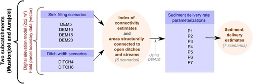
These computations (IC, sediment delivery, and connected areas) were subjected to sensitivity analyses to explore the variability of the results due to uncertain model parameters in the IC and sediment delivery computations. The data and the methods are schematically summarised in Figure 1 and described in more detail below. The results were analyzed at the pixel scale and field parcel scale, and the results between the two subcatchments are compared.

Figure 1. Schematic overview of the utilised data and the conducted scenarios and computations.

While the computations were conducted at the pixel scale (2 × 2 m²), the results were spatially aggregated to the parcel scale. The aggregation of the IC and erosion values was conducted by calculating their mean values for each parcel. Parcel scale sediment delivery was calculated as the sum of delivered sediment mass from each pixel within a parcel divided by the area of the parcel. The results are interpreted using standard statistical metrics, namely Pearson correlation and Spearman rank correlation. Pearson correlation is applied to provide quantitative insight into the relationship between variables. Spearman correlation is used to provide information particularly on the dependence between the rankings of variables at the parcel scale. The ranking of the variables is of practical interest at the parcel scale since agricultural management choices are conducted at that scale.

Catchment characteristics and field parcel data

The study area consists of two subcatchments of Mustionjoki (60.5325°N, 22.4371°E) and Aurajoki (60.1232°N, 23.7409°E) in southwestern Finland draining directly into the Baltic Sea (hereafter referred to as the Mustionjoki and Aurajoki subcatchments). The Mustionjoki subcatchment (116.2 km²) is dominated by clay soils (Vertic Luvic Stagnosols), with small areas of siltic and loamic soils (Stagnic Regosols) and more muddy soils (Umbric Gleysols). The Aurajoki subcatchment (146.6 km²) is located 86 km southwest of Mustiojoki, and its agricultural areas are dominated by clay soils (Vertic Luvic Stagnosols). The two subcatchments have contrasting topographic characteristics. Their key properties are summarised in Table 1.

Table 1. Key characteristics of the studied subcatchments.

	Mustionjoki	Aurajoki
Area (km^2)	116.2	146.6
Agricultural area (%)	30	34
Topography	Gently undulating	Gently flat, with steep slopes near rivers and streams
Average slope (%)	4.9	2.7
Soil type	Clay soil	Clay soil

The agriculture in both subcatchments is dominated by spring and winter cereals (about 60% of the field area) and perennial grass and hay-type crops. Typically, over 50% of the total field area has a wintertime vegetation cover (grass and hay, winter cereals or stubble) (Finnish Food Authority). The fields are commonly plowed in autumn with conventional moldboard plowing, but reduced tillage is also used. Riparian buffer strips are a common practice for reducing sediment and nutrient loading to surface waters, particularly at the Aurajoki subcatchment. The agricultural lands of the subcatchments are artificially well drained. That is, individual field parcels are generally surrounded by open ditches and drained by subsurface drains.

The field parcel borders for the Aurajoki and Mustionjoki subcatchments were taken from the field parcel data of the Finnish Food Authority, which contains over one million vectorised field parcels for the whole of Finland, accounting for nearly all agricultural land. According to the field parcel data, the Aurajoki subcatchment has 1766 field parcels with an average size of 2.8 ha (standard deviation 3.8 ha), and the Mustionjoki subcatchment has 1009 field parcels with an average size of 3.4 ha (standard deviation 4.9 ha).

Digital elevation models, disconnectivity elements, connected areas and related scenarios

The digital elevation model for the Aurajoki and Mustionjoki subcatchments was taken from a 2 × 2 m² resolution LiDAR-based digital elevation model (DEM) of Finland (National Land Survey of Finland 2020). The dataset is based on aerial laser scanning with point density of at least 0.5 points per square metre, providing a comprehensive spatial description of spatial elevation variation. According to the DEM product quality model, the root mean square error (RMSE) of the elevation data is guaranteed to be less than 0.3 m on slopes having the maximum steepness of 47% (National Land Survey of Finland 2017). In an external quality testing, the RMSEs of the DEM have been shown to be on average as low as 0.11 m and even lower on the mildest slopes (Oksanen 2013). RMSEs higher than 0.3 m were found only on very steep slopes covering 1.5% of the study area of the test (Oksanen 2013). In the current study, the terrain slopes were modest (Table 1) and only <0.1% of the area of the subcatchments had the slope ≥47%.

DEMs can include sinks (topographical depressions) of different sizes. While the sinks can markedly affect structural connectivity, small sinks in DEMs occur partly due to the noise in the data (Lane et al. 2017), and some sinks can be practically too small to induce structural disconnectivity (e.g. Turunen et al. 2020). We estimated that a threshold value between 0.05 and 0.20 m (see Supplement 1) can reasonably differentiate between sinks that can or cannot induce structural disconnectivity. Sinks with a lower depth than the threshold value were spatially sporadic small depressions with a small surface area, and larger sinks were larger local depressions controlling overland flow. Based on the estimation, filling sinks with a depth ≤0.10 m was interpreted as the most plausible scenario to exclude spurious sinks from the DEM, as it removed such sinks that had a small surface area and consequently a limited ability to induce structural disconnectivity (Supplement 1). The results of the external quality testing of the DEM (Oksanen 2013) justifies the use of the threshold value in the mildly undulating terrains. The value of 0.1 m also corresponds with such topographical variations that do not prevent runoff occurrence (Turunen et al. 2020). However, we recognise that the interpretation includes a degree of subjectivity. To understand how the sink treatment can affect our results, all IC computations were conducted using four different DEMs, including DEMs where sinks with depths of 0.05, 0.10, 0.15 and 0.20 m were filled. The sinks were filled using the FillDepression algorithm of Whitebox Geospatial Analysis Tools (Lindsay 2019). The computational scenarios are hereafter called DEM5, DEM10, DEM15, and DEM20, respectively (Figure 1). The computations with the different DEMs were considered to provide a range of plausible connectivity scenarios. Conceptually, the selected scenarios were also in line with the DEM-treatment concept of Lane et al. (2017), who suggested that removing noise from DEMS can be conducted by gradually filling sinks to a threshold where contributing areas to outlets do not considerably decrease. Note, however, that the study setup of Lane et al. (2017) differed from the current study for example in terms of DEM properties and catchment characteristics.

Locations of open ditches and streams were adopted from the field parcel data. The parcel boundaries typically closely match with the open ditch lines (or streams) in the landscape. The ditch and stream locations were used when computing the share of the field area connected to them. That is, in the DEMs, the ditches and streams were represented by those pixels that were located adjacent to the field parcel boundaries. The proportion of the areas that were structurally connected to open ditches and streams was estimated based on the DEM-based flow direction (the D8 algorithm) and flow accumulation computation using ArcGIS software (e.g. Kebede et al. 2021). To consider the sensitivity of the results due to possible variations in the width of the open ditches, we conducted computational scenarios where the ditch widths were extended by 4 and 6 m. That is, in these scenarios, the ditches were widened by two or three pixels, respectively, to analyze how variability in their widths and possible inaccuracies in their locations can affect our results. These scenarios are hereafter called DITCH4 and DITCH6 (Figure 1), respectively.

RUSLE data

RUSLE data for the subcatchments were taken from the existing national dataset (Räsänen 2021; Räsänen et al. in review). The dataset is based on the method of Renard et al. (1997): (1) $A=R\times K\times LS\times C\times P$(1) where A is the annual average erosion (t ha⁻¹ yr⁻¹), R is the rainfall-runoff erosivity factor (MJ mm ha⁻¹ h⁻¹ yr⁻¹), K is the soil erodibility factor (t ha h ha⁻¹ MJ⁻¹ mm⁻¹), LS is the slope length and steepness factor (−), C is the cover-management factor (−), and P is the support practice factor (−).

The dataset includes only the R, K and LS factors, and it is calculated for all agricultural lands of Finland at a two-metre resolution. In the dataset, the R factor is from a 1 km resolution gridded European scale dataset that is based on observational data (Panagos, Ballabio et al. 2015), where the R data for Finland was calculated from hourly precipitation data measured at 64 stations during the years 2007–2013. Based on this, the R-value for Aurajoki and Mustionjoki are 360 and 314 MJ mm ha⁻¹ t⁻¹yr⁻¹, respectively, while the national average is 273 MJ mm ha⁻¹ h⁻¹ yr⁻¹ with annual average precipitation of 660 mm.

The K factor is from the Finnish Soil Database (Lilja and Nevalainen 2006; Lilja, Uusitalo et al. 2017), which was supplemented with soil-specific K values (Lilja, Hyväluoma et al. 2017; Lilja, Puustinen et al. 2017). The soil database contains vector data (1:200,000) describing the Finnish soils classified according to the World Reference Base for Soil Resources (IUSS Working Group WRB 2015) with the smallest spatial feature of 6.25 ha. According to this data, the dominating agricultural soils at the Aurajoki and Mustionjoki subcatchments – Vertic Luvic Stagnosols (clay) and Stagnic Regosols (sand, silt, and loam) – have K values of 0.040 and 0.057 t ha h ha⁻¹ MJ⁻¹ mm⁻¹, respectively.

The LS is calculated from the two-metre resolution LiDAR-based digital elevation model (DEM) of Finland (National Land Survey of Finland 2020) by using the method of Desmet and Govers (1996) in the SAGA GIS module LS factor (Conrad 2003). The method computes the LS value for each grid cell by estimating the slope steepness (S) and substituting the original slope length (L) (Foster and Wischmeier 1974) with the unit contributing area, which in turn is calculated using a multiple flow direction algorithm (Quinn et al. 1991). The data for Finland uses default settings of the SAGA GIS module LS factor (rill/interrill erosivity ratio = 1 and stability = stable). The field borders were considered according to the field parcel data from the Finnish Food Authority. According to the data, the average LS value of agricultural lands of Aurajoki and Mustionjoki are 0.470 and 0.830, respectively.

In the current study, all fields were considered under uniform crop cover and management to facilitate comparability between the structural connectivity of the field parcels and the two subcatchments. Spring cereals are the most common crops in Finland, and we used the corresponding C factor value of 0.211 (spring cereals with autumn plowing) (Räsänen et al., in review).

Connectivity index computations

Following Borselli et al. (2008), the index of connectivity (IC [−]) at each pixel was computed based on an upslope (D_up [−]) and downslope (D_down [−]) factor: (2) $IC=lo{g}_{10}\left({\displaystyle \frac{D_{up}}{D_{down}}}\right)$(2) Low IC values denote areas with a lower degree of connectivity compared to higher IC values. D_up is computed as: (3) $D_{up}=\overline{WS}\sqrt{A}$(3) where $\overline{W}$ [−] is the average weighing factor for the upslope area, $\overline{S}$ [m m⁻¹] is the average terrain slope of the upslope area, and A [m²] is the upslope area. D_down is calculated as follows: (4) $D_{down}=\sum _{i=1}^n{\displaystyle \frac{d_i}{W_i{S}_i}}$(4) where n is the total number of pixels along the downslope flowpath, d_i [m] is the length of the ith pixel along the downslope flowpath (2.0 m or 2.8 m, depending on the direction of flow in the eight-direction model), W_i [−] is the weighing factor of the ith pixel, and S_i [m m⁻¹] is the terrain slope of the ith pixel. W_i describes local conditions affecting connectivity and thus relates to vegetation cover and land use. W_i was given the parameter value of the RUSLE C factor (Borselli et al. 2008), which is considered to provide an integrated description of vegetation cover and farming practices. The downslope flowpath was calculated from every pixel to the ditches and streams surrounding the field parcel.

Sediment delivery computations

Based on the computed IC values, we estimate sediment delivery rate (SDR) with a sigmoid-type function as follows (e.g. Vigiak et al. 2012; Hamel et al. 2017; Zhao et al. 2020): (5) $SD{R}_i=SD{R}_{max}{(1+\exp \left({\displaystyle \frac{I{C}_0-I{C}_i}{K_{IC}}}\right))}^{-1}$(5) where SDR_max [−] is the maximum SDR (ranging from 0 to 1.0), IC_i [−] is the computed IC value at the ith pixel, IC₀ [−], and K_IC [−] are empirical parameters. Sediment delivery is consequently estimated as (e.g. Zhao et al. 2020): (6) $Q_p={\displaystyle \frac{{\sum }_{i=1}^N{E}_{i}SD{R}_i}{a_p}}$(6) where Q_p [t ha⁻¹ yr⁻¹] is the sediment delivery via surface runoff from field parcel p, N is the total number of pixels in the field parcel, E_i [t yr⁻¹] is the erosion (RUSLE data) in the ith pixel, and a_p [ha⁻¹] is the area of the field parcel. Thus, the resulting pixel scale SDR_i values describe the share of erosion that is delivered from a pixel to the ditches and streams that surround the field parcel containing the pixel. Consequently, the Q_p values describe the amount of sediment that is delivered from a parcel to the ditches and streams.

We explored the sensitivity of the results to the parameter variation (IC₀ and K_IC) of Equation (5) by identifying different parameterizations from the literature and using local data (hereafter called P1–P7, Table 2, and Figure 1). Since sediment yield observations at the parcel scale are rare, we explored the sensitivity of the results using a wide range of possible parameterizations. P1 was set according to a widely applicable parameterisation that was previously used globally in different locations (Vigiak et al. 2012; Hamel et al. 2015; Zhao et al. 2020) and therefore may be applicable to different landscapes. P2–P4 represented a range of different parameterizations used in different locations globally (see Hamel et al. 2017) and were considered to represent a wide but possible variability in the parameter values.

Table 2. The applied parameterizations for the sensitivity analyses regarding the sediment delivery rate calculations (Equation 5).

Parameterisation	IC0	KIC	Description
P1	0.5	2.0	Widely used parameterisation
P2	0.5	1.8	Literature value
P3	0.5	3.5	Literature value
P4	0.1	2.0	Literature value
P5	−4.7	1.0	Reflects local data
P6	−3.3	1.0	Reflects local data
P7	−5.7	1.0	Reflects local data

P5–P7 were set to reflect local conditions in Finland, as follows. Sediment load via surface runoff has been observed to vary between 10% and 50% of the total load (defined as the sum of the load via surface runoff and subsurface drains) (Turtola et al. 2007; Warsta et al. 2014; Turunen et al. 2017; Finnish Environment Institute 2019). Furthermore, our preliminary computations showed median IC values of −5.2 in the studied areas. Therefore, the parameterizations P5–P7 were consequently determined by setting the SDR value at the median IC to 0.3, 0.1, and 0.5 (reflecting the typical range of surface runoff load shares from previous studies) in the parameterizations P5, P6, and P7, respectively. See Figure 2 for details. The parameterizations P5–P7 were considered to reasonably reflect the previously observed shares (10%–50%) of sediment transport via surface runoff in local conditions. Note also that while sediment is eroded on the field surface in the local conditions (Uusitalo et al. 2001), it can thereafter be efficiently transported forward via overland flow or through the soil to subsurface drains (e.g. Turtola et al. 2007; Turunen et al. 2017). While Equation (5) describes the share of eroded material that is transported by surface runoff from a pixel to open ditches and streams, the rest of the sediment is considered be either deposited on the soil surface or transported to the subsurface flow pathways. While our study focuses on the share of sediment transported by surface runoff, conceptually the parameterisation is in line with previous empirical studies.

Figure 2. Surface runoff sediment delivery rate as a function of the index of connectivity with the applied parameterizations P1–P7.

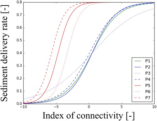
The resulting parameterizations and related sources are shown in Table 2. For all of the parametrizations (P1–P7), the SDR_max (Equation 5) was set to the widely applied value of 0.8 (Hamel et al. 2015; Liu et al. 2020; Gashaw et al. 2021; Duan et al. 2022). The consequent relationship between each parameterisation and IC values is shown in Figure 2. The sediment delivery computations were conducted using DEM10 (see Figure 1).

Results

Pixel-scale IC and erosion values and areas structurally connected to open ditches and streams

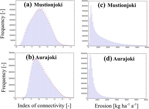
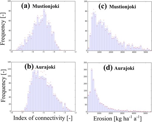
The computed IC values varied from −8.6 to −1.2 (median = −6.0 … −5.9, standard deviation σ = 1.1) in the Mustionjoki subcatchment and from −8.1 to −0.4 (median = −5.9 … −5.8, σ = 1.0–1.1) in the Aurajoki subcatchment. Their pixel scale distributions were centred around the median values and were slightly positively skewed (Figure 3a–b). Differences between the computational scenarios (DEM5–20 and DITCH4–6, Figure 1) and between the subcatchments were clearly smaller than the variability within the subcatchments (Figure 3a–b). At the Mustionjoki subcatchment, there was a wider range of IC values between the low end and the median of the distribution compared to the corresponding distribution of the Aurajoki subcatchment (Figure 3a–b), reflecting differences in catchment topographical properties. The IC distributions clearly differed from the erosion distributions (Figure 3a–d). However, there was a statistically significant relationship between the IC and logarithmic (base 10) erosion values at both of the subcatchments (Pearson r = 0.58–0.59, p < 0.01 at the Mustionjoki subcatchment and r = 0.63, p < 0.01 at the Aurajoki subcatchment), demonstrating a degree of spatial correspondence between the two spatial variables.

Figure 3. Distribution of pixel scale (a–b) index of connectivity (IC) and (c–d) erosion values at the Mustionjoki and Aurajoki subcatchments. The red lines denote the minimum and the maximum from the different computational scenarios (DEM5–20 and DITCH4–6). The low IC values denote areas with a lower degree of connectivity compared to higher IC values.

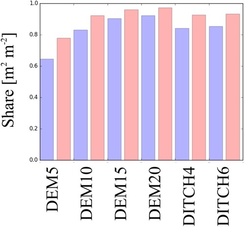
Our analysis with the different DEM treatment and ditch width scenarios (Figure 1) showed that the majority of the field area (65%–92% and 78%–97% at the Mustionjoki and Aurajoki subcatchments, respectively) was structurally connected to the adjacent ditches (Figure 4). These results on the degree of connectivity were more sensitive to the computational scenarios at the Mustionjoki subcatchment than at Aurajoki subcatchment (Figure 4).

Figure 4. The share of field area connected to open ditches and streams from the total field area with the six different computational scenarios. The blue and red bars denote the share at Mustionjoki and Aurajoki subcatchments, respectively.

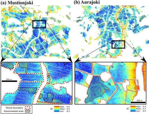
The disconnected field areas were sporadically located in the landscape and were mostly due to local depressions (Figure 5a–b). The connectivity pathways were dominated by spatially sporadic flow accumulation networks, controlled by elevation differences in the model (Figure 5a–b). At the Aurajoki subcatchment the most connected areas were concentrated near to the Aurajoki stream (Figure 5b), while at Mustionjoki, they were distributed more evenly in the landscape (Figure 5a).

Parcel scale IC and erosion values

Regarding parcel scale, the distributions of the connected mean IC values were skewed (Figure 6a–b) and differed from those of the mean parcel scale erosion values (Figure 6c–d). There was a statistically significant relationship between the mean IC and logarithmic (base 10) erosion values at the Mustionjoki subcatchment (Pearson r = 0.49, p < 0.01), and the relationship was stronger at the Aurajoki subcatchment (r = 0.67–68, p < 0.01).

Figure 6. Distribution of the mean parcel scale (a–b) index of connectivity and (c–d) erosion values at the two subcatchments. The red lines denote the minimum and maximum.

There was also a significant rank correlation between the mean parcel scale IC and erosion values at the Mustionjoki (Spearman r_s = 0.49–0.51, p < 0.01) and Aurajoki (Spearman r_s = 0.60–0.67, p < 0.01) subcatchments. As demonstrated in Figure 7a–b, the parcels with the highest mean erosion values often corresponded with the highest mean IC values. However, the relationship was not as straightforward regarding the mid-range values (Figure 7a–b).

Figure 7. A representative snapshot of (a–b) the spatial distribution of the mean parcel scale index of connectivity (IC) and (c–d) erosion [kg ha⁻¹ a⁻¹] values at the Mustionjoki and Aurajoki subcatchments.

Sediment delivery computations

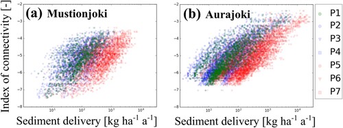
The parcel scale SDR values (parameterizations P1–P7) varied widely, ranging from 0.01 to 0.72 at the Mustionjoki subcatchment and from 0.01 to 0.74 at the Aurajoki subcatchment. Regarding the computed parcel scale sediment delivery, the estimates with different parameterizations (P1–P7) varied by several orders of magnitude (Figure 8a–b), demonstrating the high sensitivity of the delivery estimates to the parameter variations (Table 2). The mean parcel scale deliveries and logarithmic (base 10) erosion values correlated significantly at the Mustionjoki (Pearson r ≥ 0.92, p < 0.01) and Aurajoki (Pearson r ≥ 0.99, p < 0.01) subcatchments.

Most interestingly, the rank correlations between the computed deliveries regarding all scenarios (P1–P7) were high in both of the catchments (Spearman r_s> 0.95 and p < 0.01). This demonstrates a similar ranking of the parcels in terms of sediment delivery despite differences in the computed magnitude of the deliveries.

Discussion

The computed IC value ranges in the two studied catchments overlapped, but catchment characteristics also resulted in differences in the IC distributions. Previous connectivity index computations have concentrated in areas with larger topographic variations (e.g. Borselli et al. 2008; Gay et al. 2016; Hamel et al. 2017; Ortíz-Rodríguez et al. 2017; Zhao et al. 2020), and our analysis shows how IC distributions can differ in lowland areas. The difference in the median IC between the two studied subcatchments was <1.0, and the IC values varied between −8.6 and −0.4 (median −6.0 … −5.8). Topographic variations in Finland are modest, and thus the variability in Finnish catchments can be assumed to be typically higher within catchments than between catchments. However, the variability between catchments should be analyzed by studying a larger number of catchments to reach definitive conclusions. For reference, Zhao et al. (2020) reported IC values between −10.3 and 5.4 in the Yellow River catchment area (China). Gay et al. (2016) reported mean IC values between −3.9 and 10.0 in the lowlands of France. Cantreul et al. (2018) reported median IC values between −8.0 and −6.5 in a lowland area in Belgium. Note, however, that the values from the previous studies are not directly comparable with our results, as the application differed in terms of the applied data, parameterizations, and methodological choices. However, the comparison can provide insight into the variability of connectivity within different catchments. Gay et al. (2016) also developed a model to consider infiltration and saturation processes in the IC computations, which may provide insight into more comprehensive connectivity assessments in humid lowland areas.

The correlation between the IC and RUSLE values (at the both pixel and field parcel scales) as well as between the sediment delivery and RUSLE values suggests that areas with high computed erosion also tend to be structurally well-connected to adjacent open ditches. The IC and erosion values correlated more in the Aurajoki subcatchment than in the Mustionjoki subcatchment. The difference was likely due to the clear topographical slopes adjacent to the Aurajoki stream and the more evenly distributed topographical variations in the Mustionjoki subcatchment. Previously Hamel et al. (2017) also showed that there can be a relationship between IC and sediment delivery at the catchment outlets. The RUSLE results reflect the connectivity magnitude, but the applied IC model further improves the understanding of sediment connectivity by providing quantitative estimates of the variability of connectivity in structurally varying landscapes. There was a relationship between the IC and RUSLE results particularly since the LS parameter of RUSLE (the slope length and steepness factor) and the upslope factor of the IC computations both contained information on the landscape structure upslope from each pixel. The IC computations, however, also considered the landscape structure downslope from each pixel (see Equation 4). The downslope factor did not dominate the result due to the relatively small mean area of the field parcels (mean 2.8–3.4 ha). However, we identified two cases where the relationship between erosion and connectivity was not strong. Areas with high erosion and low IC were located in regions where the downslope flow pathway was long and ran through relatively flat areas. Areas with high IC and low erosion were often located in relatively flat areas that had a relatively large upslope area and were located close to a ditch or stream.

Our analysis showed that the structural surface runoff connectivity was often dominated by spatially sporadic networks with relatively high IC values (Figure 5). Thus, while there were apparent differences between field parcels in terms of connectivity, they often had similarities in terms of spatial patterns of connectivity. Tree-like spatial connectivity structures were particularly prominent and they are often found in landscapes likely due to landscape evolution and the formation of efficient surface runoff drainage networks (e.g. Kwang et al. 2021). The results also demonstrate that the majority of agricultural land areas can be structurally connected to the adjacent open ditches and streams (in terms of surface runoff) (Figure 4). Previous field-scale studies (e.g. Uusi-Kämppä et al. 2000; Uusi-Kämppä and Jauhiainen 2010) showed that buffer strips can efficiently reduce sediment loads by mitigating erosion on steep slopes and retaining settled soil particles, but our study showed how the potential relates to a spatially larger view. Since the field parcels are connected to the adjacent ditches and streams, buffer strips can have a role in reducing sediment loads on a large scale by retaining settled soil particles if they are well-targeted and can efficiently reduce sediment loads via concentrated surface runoff fluxes. Also, so-called grassed waterways established on concentrated water flows in the field may efficiently decrease erosion and sediment load in overland flow channels. In further studies, the computational model of the current study could be applied to estimate the potential impacts of spatially targeted buffer strips, grassed waterways, and other environmental measures (e.g. wintertime vegetation cover) on sediment delivery. Practically, such analysis can be conducted by describing the effects of land cover on connectivity with the spatially distributed C and P factors of RUSLE (Equation 1) and W factor of the IC computations (Equations 3 and 4) (e.g. Foerster et al. 2014).

Figure 5. A representative snapshot of the pixel scale spatial distribution of the index of connectivity (IC) at the (a) Mustionjoki and (b) Aurajoki subcatchments. Ditches and streams surrounding the parcels are located in the same places as the parcel boundaries.

The topographic variations in the studied catchments were modest (mean slope ≤5%), which is typical in Finland. While the utilised DEM with the resolution of 2 × 2 m² represents macrotopographic features, the choices of farming practices (particularly tillage method and direction) can be assumed to have a role in controlling surface runoff. For example, contour tillage may reduce runoff and sediment loads (Jia et al. 2020). One of the practical applications of spatially distributed IC data would be the identification of those locations where contour tillage can have a high potential to control runoff and sediment load. Hypothetically, contour tillage can have a high impact on connectivity, particularly in field parcels where the spatial IC networks are connected to a ditch or stream via several different locations throughout a hillslope (i.e. the surface runoff fluxes are not too concentrated to constantly increase the flow depth above the tillage furrows).

While the studied differences in the sediment delivery parameterizations (Equation 5, Figure 2) resulted in widely varying sediment delivery magnitudes, the rank correlation between the parcel-scale deliveries with the different scenarios was high (Spearman r_s> 0.95). This means that despite the differences in the delivery magnitudes, the different parameterizations resulted in a similar ranking of the field parcels (in terms of sediment deliveries). This capability of the model to produce consistent estimates to discern which field parcels can potentially have both high erosion and high connectivity values can be practically interesting from the point of view of targeting sediment load mitigation measures. However, regarding the sediment delivery magnitudes and choice of related parameterizations, our study did not reach any conclusions. Previously Hamel et al. (2015), who studied sediment export in North Carolina (US), also showed that the applied computational approach can be a useful tool in ranking sediment transport areas and prioritising the targeting of environmental measures.

It is also noteworthy that in addition to surface runoff, comprehensive sediment connectivity assessments should consider subsurface sediment delivery. Soil particles eroded on the soil surface can be vertically transported particularly to subsurface drains and, thereafter, directly to adjacent surface water (Øygarden et al. 1997; Uusitalo et al. 2001; Foster et al. 2003; Turtola et al. 2007; Turunen et al. 2017), bypassing any disconnectivity elements on the soil surface. Our approach considers only structural sediment connectivity via surface runoff. The applied approach has been tested in several studies and different data (e.g. Borselli et al. 2008; Hamel et al. 2017; Zhao et al. 2020). According to physics-based surface runoff models (e.g. Taskinen and Bruen 2007) terrain elevation difference is a primary factor controlling runoff routing. Thus, the concept of structural connectivity via surface runoff is well-justified. However, studying connectivity dynamics, for example, with dynamic sediment delivery simulations (e.g. Warsta et al. 2014) would further improve the understanding of how connectivity can vary in space and time. Consideration of infiltration processes (e.g. Gay et al. 2016) could also further improve our estimate but would require consideration of factors such as soil hydraulic properties and subsurface drainage parameters. Also, calibration and validation of the sediment delivery rate equation (Equation 5, Figure 2) with local data would further improve the accuracy of the results.

Despite the involved uncertainties and limitations, our analysis provides the first large-scale sediment connectivity analysis in the agricultural lands of Finland. The approach also involved an exploration of the sensitivity of the results to key uncertainties (Figure 1). The exploration showed that the key results are not highly sensitive to variation in the studied variables. Note, however, that while the ranking of the field parcels according to sediment delivery was not highly sensitive to the parameter variations, the sediment delivery magnitudes were very sensitive to the variations (Figure 8). The practicality of our approach is highlighted by the fact that the computations can be extended to the national scale in Finland, as the digital elevation models and RUSLE data are already openly available (Räsänen 2021). Generating open spatial data on sediment connectivity would increase the possibilities to predict potential sediment connectivity pathways and consequently provide systems-based information to enhance discussion regarding the targeting of sediment mitigation measures (e.g. buffer strips) on the field surface. The data could be further extended with spatially and temporally distributed parameterisation of the modelling approach (e.g. Foerster et al. 2014), which would provide a tool to produce estimates regarding the impacts of different water protection measures on sediment connectivity.

Figure 8. Relationship between the computed mean parcel scale sediment deliveries and connectivity indices at the (a) Mustionjoki and (b) Aurajoki subcatchments with the applied parameterizations P1–P7.

Acknowledgments

This project was funded by the EJP SOIL SCALE project. The project has received funding from the European Union’s Horizon 2020 research and innovation programme: Grant agreement No 862695. The project made use of data and geocomputing resources provided by CSC – IT Center for Science, Finland (urn:nbn:fi:research-infras-2016072531) and the Open Geospatial Information Infrastructure for Research (Geoportti RI, urn:nbn:fi:research-infras-2016072513).

Disclosure statement

No potential conflict of interest was reported by the author(s).

Additional information

Funding

This project was funded by the EJP SOIL SCALE project. The project has received funding from the European Union's Horizon 2020 research and innovation programme: Grant agreement No 862695.

Notes on contributors

M. Tähtikarhu

Mika Tähtikarhu is a researcher at Natural Resources Institute Finland. His research interests are related to hydrology, soil and modeling.

T. Räsänen

Timo Räsänen is a senior researcher at Natural Resources Institute Finland. His research interests are related to hydrology, erosion, water management, climatic variability and modeling.

J. Oksanen

Juha Oksanen is the director of the Department of Geoinformatics and Cartography at Finnish Geospatial Research Institute in the National Land Survey of Finland. He is an expert in geocomputing and geovisualisation. He has extensive experience in DEM uncertainty modelling and is among the pioneers bringing LiDAR-based DEM production in Finland in early 2000.

J. Uusi-Kämppä

Jaana Uusi-Kämppä is a senior researcher at Natural Resources Institute Finland. Her research interests are related to buffer zones, mitigation of water pollution and transport of glyphosate and AMPA in soil and water.

References

- Borselli L, Cassi P, Torri D. 2008. Prolegomena to sediment and flow connectivity in the landscape: a GIS and field numerical assessment. Catena. 75(3):268–277.
- Cantreul V, Bielders C, Calsamiglia A, Degré A. 2018. How pixel size affects a sediment connectivity index in central Belgium. Earth Surf Processes Landforms. 43(4):884–893.
- Conrad O. 2003. SAGA-GIS module library documentation (v2.2.0) [WWW document]. System of Automated Geoscientific Analyses (SAGA). [accessed 2021 June 8]. http://www.saga-gis.org/saga_tool_doc/2.2.0/ta_hydrology_22.html.
- Desmet PJJ, Govers G. 1996. A GIS Procedure for Automatically Calculating the USLE LS Factor on Topographically Complex Landscape Units. J Soil Water Conserv. 51(5):427–433.
- Duan T, Feng J, Chang X, Li Y. 2022. Watershed health assessment using the coupled integrated multistatistic analyses and PSIR framework. Sci Total Environ. 847:157523.
- Finnish Environment Institute. 2019. Sediment and nutrient loading to surface waters in 3 different scales [WWW document]. Finnish Environment Institute (SYKE). [accessed 2021 Jan 25]. https://metasiirto.ymparisto.fi:8443/geoportal/catalog/search/resource/details.page?uuid=%7B15893DD0-0193-40AD-9E21-452D271DB791%7D.
- Foerster S, Wilczok C, Brosinsky A, Segl K. 2014. Assessment of sediment connectivity from vegetation cover and topography using remotely sensed data in a dryland catchment in the Spanish Pyrenees. J Soils Sediments. 14(12):1982–2000.
- Foster GR, Wischmeier W. 1974. Evaluating irregular slopes for soil loss prediction. Trans ASAE. 17(2):305–0309.
- Foster IDL, Chapman AS, Hodgkinson RM, Jones AR, Lees JA, Turner SE, Scott M. 2003. Changing suspended sediment and particulate phosphorus loads and pathways in underdrained lowland agricultural catchments; Herefordshire and Worcestershire, U.K. The Interactions Between Sediments and Water. 119–126. doi:10.1007/978-94-017-3366-3_17.
- Fresne M, Jordan P, Daly K, Fenton O, Mellander PE. 2022. The role of colloids and other fractions in the below-ground delivery of phosphorus from agricultural hillslopes to streams. Catena. 208:105735.
- Garcia-Ruiz JM, Beguería S, Nadal-Romero E, Gonzalez-Hidalgo JC, Lana-Renault N, Sanjuán Y. 2015. A meta-analysis of soil erosion rates across the world. Geomorphology. 239:160–173.
- Gashaw T, Bantider A, Zeleke G, Alamirew T, Jemberu W, Worqlul AW, Dile YT, Bewket W, Meshesha DT, Adem AA, Addisu S. 2021. Evaluating InVEST model for estimating soil loss and sediment export in data scarce regions of the Abbay (Upper Blue Nile) basin: implications for land managers. Environmental Challenges. 5:100381.
- Gay A, Cerdan O, Mardhel V, Desmet M. 2016. Application of an index of sediment connectivity in a lowland area. J Soils Sediments. 16(1):280–293.
- Hamel P, Chaplin-Kramer R, Sim S, Mueller C. 2015. A new approach to modeling the sediment retention service (InVEST 3.0): case study of the Cape Fear catchment, North Carolina, USA. Sci Total Environ. 524-525:166–177.
- Hamel P, Falinski K, Sharp R, Auerbach DA, Sánchez-Canales M, Dennedy-Frank PJ. 2017. Sediment delivery modeling in practice: comparing the effects of watershed characteristics and data resolution across hydroclimatic regions. Sci Total Environ. 580:1381–1388.
- IUSS Working Group WRB. 2015. World reference base for soil resources 2014, update 2015. International soil classification system for naming soils and creating legends for soil maps (No. 106), World soil resources reports. Rome: FAO.
- Jia L, Zhao W, Zhai R, An Y, Pereira P. 2020. Quantifying the effects of contour tillage in controlling water erosion in China: a meta-analysis. Catena. 195:104829.
- Kebede YS, Endalamaw NT, Sinshaw BG, Atinkut HB. 2021. Modeling soil erosion using RUSLE and GIS at watershed level in the upper Beles, Ethiopia. Environmental Challenges. 2:100009.
- Kwang JS, Langston AL, Parker G. 2021. The role of lateral erosion in the evolution of nondendritic drainage networks to dendricity and the persistence of dynamic networks. Proc Natl Acad Sci USA. 118(16):e2015770118.
- Lane SN, Bakker M, Gabbud C, Micheletti N, Saugy JN. 2017. Sediment export, transient landscape response and catchment-scale connectivity following rapid climate warming and alpine glacier recession. Geomorphology. 277:210–227.
- Lilja H, Hyväluoma J, Puustinen M, Uusi-Kämppä J, Turtola E. 2017. Evaluation of RUSLE2015 erosion model for boreal conditions. Geoderma Regional. 10:77–84. doi:10.1016/j.geodrs.2017.05.003.
- Lilja H, Nevalainen R. 2006. Chapter 5 developing a digital soil map for Finland. In: Lagacherie P, McBratney AB, Voltz M, editors. Developments in soil science, digital soil mapping. Elsevier; p. 67–603. doi:10.1016/S0166-2481(06)31005-7.
- Lilja H, Puustinen M, Turtola E, Hyväluoma J. 2017. Suomen peltojen karttapohjainen eroosioluokitus (Map-based classificication of erosion in agricultural lands of Finland). Natural Resources Institute Finland (Luke). 36:1–68.
- Lilja H, Uusitalo R, Yli-Halla M, Nevalainen R, Väänänen R, Tamminen P, Tuhtar J. 2017. Suomen maannostietokanta: Käyttöopas versio 1.1 (Finnish Soil Database: Manual, version 1.1) (No. 6), Luonnonvara- ja biotalouden tutkimus. Luonnonvarakeskus (LUKE) (Natural Resources Institute Finland).
- Lindsay J. 2019. FillDepressions algorithm of Whitebox geospatial analysis tools. WhiteboxTools User Manual. [accessed 2022 Dec 9]. https://www.whiteboxgeo.com/manual/wbt_book/.
- Liu H, Liu Y, Wang K, Zhao W. 2020. Soil conservation efficiency assessment based on land use scenarios in the Nile River Basin. Ecol Indic. 119:106864.
- López-Vicente M, Poesen J, Navas A, Gaspar L. 2013. Predicting runoff and sediment connectivity and soil erosion by water for different land use scenarios in the Spanish pre-Pyrenees. Catena. 102:62–73.
- McKay LD, Gillham RW, Cherry JA. 1993. Field experiments in a fractured clay till: 2. Solute and colloid transport. Water Resour Res. 29(12):3879–3890.
- National Land Survey of Finland. 2017. Kansallisen maastotietokannan laatumalli – Korkeusmallit (Quality model of the national topographic database – digital elevation models) [WWW Document]. [accessed 2022 Sep 23]. https://www.maanmittauslaitos.fi/sites/maanmittauslaitos.fi/files/attachments/2017/05/KMTK_korkeusmallit_laatukasikirja_2017-01-02.pdf.
- National Land Survey of Finland. 2020. Elevation model 2m [WWW Document]. [accessed 2020 May 29]. https://www.maanmittauslaitos.fi/en/maps-and-spatial-data/expert-users/product-descriptions/elevation-model-2-m.
- Oksanen J. 2013. Can binning be the key to understanding the uncertainty of DEMs. Proceedings of the GISRUK. 2013:3–5.
- Ortíz-Rodríguez AJ, Borselli L, Sarocchi D. 2017. Flow connectivity in active volcanic areas: Use of index of connectivity in the assessment of lateral flow contribution to main streams. Catena. 157:90–111.
- Øygarden L, Kværner J, Jenssen PD. 1997. Soil erosion via preferential flow to drainage systems in clay soils. Geoderma. 76:65–86. doi:10.1016/S0016-7061(96)00099-7.
- Panagos P, Ballabio C, Borrelli P, Meusburger K, Klik A, Rousseva S, Tadić MP, Michaelides S, Hrabalíková M, Olsen P, et al. 2015. Rainfall erosivity in Europe. Sci Total Environ. 511:801–814. doi:10.1016/j.scitotenv.2015.01.008.
- Panagos P, Borrelli P, Poesen J, Ballabio C, Lugato E, Meusburger K, Montanarella L, Alewell C. 2015. The new assessment of soil loss by water erosion in Europe. Environ Sci Policy. 54:438–447.
- Puustinen M, Turtola E, Kukkonen M, Koskiaho J, Linjama J, Niinioja R, Tattari S. 2010. VIHMA—a tool for allocation of measures to control erosion and nutrient loading from Finnish agricultural catchments. Agric Ecosyst Environ. 138(3-4):306–317.
- Quinn PFBJ, Beven K, Chevallier P, Planchon O. 1991. The prediction of hillslope flow paths for distributed hydrological modelling using digital terrain models. Hydrol Processes. 5(1):59–79.
- Räsänen TA. 2021. The erosion susceptibility of Finnish agricultural lands [Data set]. Natural Resources Insitute Finland (LUKE). Data available at Paituli: http://urn.fi/urn:nbn:fi:att:fdb14fe3-dd2d-499f-81a5-e1e799d8db8a.
- Räsänen TA, Tähtikarhu M, Uusi-Kämppä J, Piirainen S, Turtola E. under review. Evaluation of RUSLE and spatial assessment of agricultural erosion in Finland. Geoderma Regional.
- Renard KG, Foster GR, Weesies GA, McCool DK, Yoder DC. 1997. Predicting soil erosion by water: a guide to conservation planning with the revised universal soil loss equation (RUSLE). Agricultural Handbook 703. Washington (DC): US Department of Agriculture; p. 404.
- Taskinen A, Bruen M. 2007. Incremental distributed modelling investigation in a small agricultural catchment: 1. Overland flow with comparison with the unit hydrograph model. Hydrol Processes. 21(1):80–91.
- Turtola E, Alakukku L, Uusitalo R. 2007. Surface runoff, subsurface drainflow and soil erosion as affected by tillage in a clayey Finnish soil. AFSci. 16:332–351. doi:10.2137/145960607784125429.
- Turunen M, Turtola E, Vaaja MT, Hyväluoma J, Koivusalo H. 2020. Terrestrial laser scanning data combined with 3D hydrological modeling decipher the role of tillage in field water balance and runoff generation. Catena. 187:104363.
- Turunen M, Warsta L, Paasonen-Kivekäs M, Koivusalo H. 2017. Computational assessment of sediment balance and suspended sediment transport pathways in subsurface drained clayey soils. Soil and Tillage Research. 174:58–69. doi:10.1016/j.still.2017.06.002.
- Ulén B. 2004. Size and settling velocities of phosphorus-containing particles in water from agricultural drains. Water, Air, Soil Pollut. 157(1):331–343.
- Ulén B, Bechmann M, Øygarden L, Kyllmar K. 2012. Soil erosion in Nordic countries–future challenges and research needs. Acta Agriculturae Scandinavica, Section B–Soil & Plant Science. 62(Supp. 2):176–184.
- Uusi-Kämppä J, Braskerud B, Jansson H, Syversen N, Uusitalo R. 2000. Buffer zones and constructed wetlands as filters for agricultural phosphorus. J Environ Qual. 29(1):151–158.
- Uusi-Kämppä J, Jauhiainen L. 2010. Long-term monitoring of buffer zone efficiency under different cultivation techniques in boreal conditions. Agric Ecosyst Environ. 137(1–2):75–85.
- Uusitalo R, Turtola E, Kauppila T, Lilja T. 2001. Particulate phosphorus and sediment in surface runoff and drainflow from clayey soils. J Environ Qual. 30:589–595. doi:10.2134/jeq2001.302589x.
- Vigiak O, Borselli L, Newham LTH, McInnes J, Roberts AM. 2012. Comparison of conceptual landscape metrics to define hillslope-scale sediment delivery ratio. Geomorphology. 138(1):74–88.
- Wainwright J, Turnbull L, Ibrahim TG, Lexartza-Artza I, Thornton SF, Brazier RE. 2011. Linking environmental regimes, space and time: interpretations of structural and functional connectivity. Geomorphology. 126(3-4):387–404.
- Warsta L, Taskinen A, Paasonen-Kivekäs M, Karvonen T, Koivusalo H. 2014. Spatially distributed simulation of water balance and sediment transport in an agricultural field. Soil and Tillage Research. 143:26–37.
- Zhao G, Gao P, Tian P, Sun W, Hu J, Mu X. 2020. Assessing sediment connectivity and soil erosion by water in a representative catchment on the Loess Plateau, China. Catena. 185:104284.