Drone-mounted UWB snow radar: technical improvements and field results

Abstract

Drone borne radar systems have seen considerable advances over recent years, and the application of drone-mounted continuous wave (CW) radars for remote sensing of snow properties has great potential. Regardless, major challenges remain in antenna design for which both low weight and small size combined with high gain and bandwidth are important design parameters. Additional limiting factors for CW radars include range ambiguities and antenna isolation. To solve these problems, we have developed an ultra-wideband snow sounder (UWiBaSS), specifically designed for drone-mounted measurements of snow properties. In this paper, we present the next iteration of this prototype radar system, including a novel antenna configuration and useful processing techniques for drone borne radar. Finally, we present results from a field campaign on Svalbard aimed to measure snow depth distribution. This radar system is capable of measuring snow depth with a correlation coefficient of 0.97 compared to in situ depth probing.

Keywords:

• UWB radar
• antenna design
• UAV
• snow

1. Introduction

A complete understanding of the Arctic cryosphere has historically been hindered by its large extent, remoteness, and restrictions in measurement methods and equipment. Remote sensing provides methods for observing the snow cover through indirect measurement and parameter estimation. For instance, ice extent is often estimated without direct verification [1,2], but many cryospheric properties including snow thickness or density require direct measurement for calibration and validation [3]. In cryospheric data collection, such as snow pits and ice core extraction, sample site selection and sample size are limited by weather, safety concerns, marine navigability as well as snow or ice thickness, convenience, and accessibility. Therefore, it is of interest to study the application of unmanned aerial vehicle (UAV)-based radar, which could offer efficient, non-invasive, and continuous field data collection of cryospheric data. This includes snow depth and stratigraphy, potentially expanding datasets used for modeling, or used directly as a data product.

In the context of remote sensing of snowpack parameters, the microwave response from snow is determined by snowpack parameters (depth, density, liquid water content, layering, crystal structure, temperature, surface roughness) and radar parameters (range, frequency, incidence angle). Therefore, ground truth data are often required to verify or calibrate measurements. As such, the success of indirect data collection for calibration and validation relies on the ability of the data acquisition device to measure these properties.

This study focuses on the indirect measurement of snow thickness and stratigraphy with high precision, where, in the case of dry snow, the main contributing element for such measurements is snow density. Snow density directly influences the dielectric constant of snow [4], which in turn influences the reflection of the radar signal. Snow density is currently manually measured, but future work includes a study with the aim to develop methods for extracting this parameter directly from radar measurements.

The UWiBaSS discussed in this paper is a ground-penetrating radar system developed for drone-mounted operations. A preceding iteration of this radar system was presented in [5].

Previous studies show that ultra wide-band (UWB) radars are able to measure snow depth and even stratigraphy with high accuracy. For instance, an 8–18 GHz frequency modulated continuous wave (FMCW) system was found to generate stratigraphic snow information with a correlation coefficient, C, of 0.92 relative to in situ depth measurements up to snow depths of 30 cm [6], while other studies show similar, but smaller, correlations: C = 0.86 [7], and C = 0.78 [8]. Nevertheless, one should note that high correlations are achieved, however, only at shallow snow depths up to 30 cm. A recent study demonstrates a lightweight FMCW Ku-band (14–16 GHz) radar for snowpack remote sensing [9]. Additionally, a gated step-frequency ground penetrating radar (GPR), operating in the 0.5–3 GHz range, enables snow and ice measuring capabilities to a depth of 11 m, operated from a snowmobile platform [10]. Moreover, it has previously been shown that aircraft-mounted radar systems are also capable of measuring snow depth with C = 0.88 in situ correlation [11], while other radar systems demonstrate snow interface detection [12], or even both snow and ice interface detection [13]. Another paper established design parameters for a UAV mounted radar intended for snow parameter retrieval [14], with a recommended operating frequency in the 1.5–4.5 GHz band. Furthermore, a number of other research groups have described UWB radars for UAV mounting, where the applications range from detection of ground targets such as cars, humans [15,16], and ships [17] as well as topographic mapping [18], detection of buried objects including landmines [19] and other high scattering targets [20]. Additionally, investigations of UAV-mounted software defined radio (SDR) GPR have previously been examined [21].

In the field of Drone-mounted synthetic aperture radar (SAR), recent studies show the possibility of landmine detection with polarimetric SAR [22] and antenna arrays for GPR systems on drones [23] which yield a wider swath when flying in grid flights, potentially extending area coverage.

This paper presents hardware and software improvements of the UWiBaSS and field results both from altitude experiments (Section 4.2) and snow measurements (Section 5).

2. Theory

Perhaps the most central quality parameters when taking snow measurements with radars are penetration depth and spatial resolution. This section will go through the limiting factors these parameters impose on radar sensing of snow.

2.1. Penetration depth

The distance an electromagnetic wave travels through a medium before its intensity is reduced by 1/e (about 37%) is referred to as the penetration depth and is used in practice to estimate how microwaves attenuate within a medium.

The EM-wave penetration depth of snow and ice is a function of radar frequency, brine volume, incident angle, temperature, density, liquid water content, snow particle diameter and conductivity of the ice or snow [24].

To determine the penetration depth, the complex dielectric constant, ε, must be known. The complex dielectric constant is defined by Daniels [25]: (1) $ϵ={ϵ}_0({ϵ}_r^{\mathrm{\prime }}-j{ϵ}_r^{\mathrm{\prime }\mathrm{\prime }}),$(1) where ${ϵ}_0$ is the free-space dielectric constant, ${ϵ}_r^{\mathrm{\prime }}$ the relative dielectric constant, and ${ϵ}_r^{\mathrm{\prime }\mathrm{\prime }}$ the relative imaginary dielectric constant. The value of ε depends on several snow state variables. Predicting the microwave response can be complicated due to the depth gradient of liquid water content and/or salinity concentration within the snowpack, in addition to the frequency dependence of all parameters. Often ε is simplified and estimated semi-empirically [24,26].

The penetration depth δ in a snow or ice medium is controlled by scattering and absorption losses. If scattering losses are assumed to be negligible, δ can be expressed as [27,28]: (2) $\delta =\frac{\lambda }{4\pi }{\left(\frac{{ϵ}_r^{\mathrm{\prime }}}{2}({[1+{\left(\frac{{ϵ}_r^{\mathrm{\prime }\mathrm{\prime }}}{{ϵ}_r^{\mathrm{\prime }}}\right)}^2]}^{1/2}-1)\right)}^{-1/2},$(2) where λ is the wavelength for free space.

Consequently the loss in the medium can be expressed as: (3) $L=10\log (e^{1/\delta })[\mathrm{dB}/\mathrm{m}].$(3) If ${ϵ}_r^{\mathrm{\prime }\mathrm{\prime }}/{ϵ}_r^{\mathrm{\prime }}\ll 1$, which usually is the case for snow, equation (2(2) $\delta =\frac{\lambda }{4\pi }{\left(\frac{{ϵ}_r^{\mathrm{\prime }}}{2}({[1+{\left(\frac{{ϵ}_r^{\mathrm{\prime }\mathrm{\prime }}}{{ϵ}_r^{\mathrm{\prime }}}\right)}^2]}^{1/2}-1)\right)}^{-1/2},$(2) ) is simplified to [27]: (4) $\delta \approx \frac{\lambda \sqrt{{ϵ}_r^{\mathrm{\prime }}}}{2\pi {ϵ}_r^{\mathrm{\prime }\mathrm{\prime }}}.$(4) Since ${ϵ}_r^{\mathrm{\prime }\mathrm{\prime }}$ of water is several orders of magnitude larger than that of dry snow, even very small amounts of liquid water in the snowpack can dramatically decrease the penetration depth δ.

The complex dielectric constant of snow and ice can be estimated using both empirical and theoretical models for the real and imaginary parts. Figure 1 shows a comparison of selected models used to calculate penetration depth. The models were collected from: [4,29–35]. The complex dielectric constant of snow has several adequate empirical models [4,31]. However, these models are limited to the low-frequency approximation (≈1 GHz) for which the effects of scattering can be neglected. This limitation implies that the low-frequency dielectric constant is not dependent on grain size. The Strong Fluctuation Model for Dry Snow [32] treats snow as a medium of randomly scattered ice particles suspended in a background medium which, in the case of snow, is air.

Figure 1. Penetration depth at a temperature of 268 K shown as a function of frequency for dry snow with 0.5 mm grain size, wet snow with dry snow density of 0.4 g/ccm, freshwater ice, and impure ice. Dry snow penetration depth is calculated with two different models, where the main difference is that the Tsang model accounts for grain size.

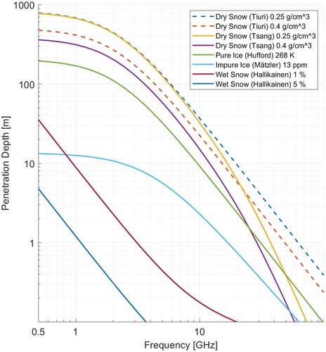
Penetration depth models for all mentioned media are depicted in Figure 1.

Generally, these media act as low pass filters in the microwave frequency range where lower frequencies penetrate deeper into the medium.

Based on the results from Figure 1, we need a radar system that operates at sufficiently low frequencies to penetrate most snow types and still have a high enough bandwidth (i.e. resolution) to resolve internal layers in the snowpack.

2.2. Resolution

The range resolution of a pulse compression radar system is given by Richards [36]: (5) $\mathrm{\Delta }r=\frac{c}{2B}\frac{1}{\sqrt{{ϵ}_r}},$(5) where B is the effective bandwidth of the radar transmitter and receiver and ${ϵ}_r$ is the complex relative dielectric constant.

Equation (5(5) $\mathrm{\Delta }r=\frac{c}{2B}\frac{1}{\sqrt{{ϵ}_r}},$(5) ) shows that the radar system bandwidth is a fundamental parameter of the range resolution and, theoretically, the only factor that can be modified to improve the range resolution significantly. For high-valued dielectric media, ${ϵ}_r$ also has a marked impact on the range resolution. In radar applications, additional factors such as pulse compression, Fourier domain windowing, and image processing methods affect the radar system output range resolution, however, only to a minor degree.

More importantly, the total bandwidth of any radar system also depends on the bandwidth of the transmitting (TX) and receiving (RX) antennas. The radar sensor used in the UWiBaSS has a bandwidth of 0.1–6 GHz, which makes the bandwidth of the antennas the main limiting factor for the total bandwidth, as all applied antenna designs have bandwidths that are sub-bands within this bandwidth of nearly 6 octaves.

The next two sections will present technical and software methods to improve on the limiting factors presented.

3. Methods: technical improvements

This section presents the recent technical improvements made to the UWiBaSS motivated by the limiting factors presented in the previous section. These improvements include antenna re-design and further radar system development that increase the versatility and usability of the UWiBaSS.

3.1. Radar system description

The radar system consists of 6 main modules:

1. Radar sensor

2. Single board computer

3. Radio modem

4. RF amplifier on TX channel

5. Antenna system

6. Power handling board, Mavlink serial connection and heating element.

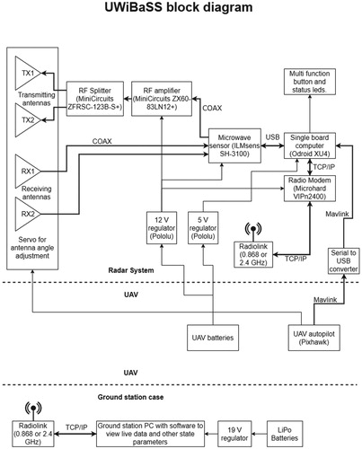
The radar system consists of an ILMsens SH-3100 radar sensor, a Minicircuits ZX60-83LN12+ amplifier for the TX channel, dual Vivaldi antennas in a bistatic configuration and an Odroid XU2 single board acquisition computer. The system is described in more detail in [5], and the new improved antenna system is described in Section 3.3 below. The integration with the UAV is illustrated in Figure 2 where the block diagram of the UWiBaSS illustrates synchronization and data transfer between the UAV autopilot as well as antenna angle regulation.

Figure 2. Block diagrams of the UWiBaSS.

The ILMsens SH-3100 UWB sensor has several desirable characteristics concerning high-resolution radar imaging.¹ Using their own developed m-sequence pseudo-random noise (PRN) signal generator, this sensor performs well for radar sensing tasks, especially when we have restrictions regarding high peaks of transmitted energy commonly associated with pulse radars. Additionally, the use of maximum length binary sequence (MLBS) allows for a single frequency oscillator, thus reducing clock jitter. The sensor has a transmitter channel and two receiver channels working in parallel.

Table 1 describes the key characteristics of the radar system. The bandwidth is the combined bandwidth of the sensor and the antennas. Thus, the resolution is the measured Full Width at Half Maximum (FWHM) distance of a processed radar pulse.

Table 1. UWiBaSS key characteristics.

Attribute	Value
Signal generation	UWB Pseudo noise
System bandwidth	3.8 GHz (0.7–4.5)
Range resolution	≈5 cm
m-sequence clock frequency	13.312 GHz
Measurement rate	52 Hz (max 1000 Hz)
MLBS order	9 (511 range bins)
Nominal output power	17.3 dBm
Unambiguous range in air	5.9 m
Average power consumption	8.1–9 W
Total Weight	≈3 kg
Transmitter
No high voltage peaks
Low field strength operation
Power splitter into Dual Vivaldi antenna prototype
Receiver
Continuous, synchronous sub-sampling operation
Timebase jitter less than 20 fs (rms)
Dual Vivaldi prototype with each antenna
Element into separate channel

The radar sensor is used in conjunction with four linearly polarized transceiving antennas mounted in pairs as RX and TX arrays, a concept described in more detail in Section 3.3.

3.2. UAV platform

The UAV used to carry the UWiBaSS is a purpose-built X8 multicopter called “Fox”. The “Fox” uses four 12 cell 88Ah Li-Po batteries and can lift a maximum payload of 25 kg. Each of the eight engines (U11, 120KV) has a maximum rated thrust of 12.3 kg using 27” propellers. For navigation and control, a “Cube Black” running “Arducopter” is used. It is set up with a “Here+” real-time kinematic (RTK) global positioning system (GPS),² providing significantly more accurate position estimates than regular GPS devices. In single-channel mode with less than 20 km distance to the base station, the positioning system has relative and absolute accuracy better than 10 cm and 1 m, respectively. Additionally, an SF11³ laser rangefinder accurately measures the distance to the ground. This also provides autonomous flights that has been used in data collection for the field campaign described in Section 5.

3.3. Antenna improvements

The UWiBaSS has been tested with several different antenna configurations: Using RX and TX spiral antennas [37], a combination of Vivaldi and spiral antennas [5] and currently dual, modified Vivaldi antennas in a bistatic configuration. With the latter configuration, we add a transversal dimension to the otherwise planar antennas. This focuses the antenna beam along the most de-focused axis (H-plane), significantly improving overall antenna directivity compared to a single element (see Figure 4). In addition to the dual antenna configuration, the Vivaldi antennas have inserted slits to shift the effective bandwidth to lower frequencies while keeping a small form factor [38]. Additionally, the antennas are modified with a printed lens in the aperture to increase gain and reduce side-lobe levels [39]. Finally, the inserted slits have also been modified with resistive loads in the opening of the slits to dissipate the current distribution occurring at the sides of the antennas. This modification reduces ringing from residual energy not radiated by the antenna at the front aperture. It was found, through simulation, that a resistor value of approximately 1 k Ω is optimal. Figure 3(a) shows a close-up photo of the modified Vivaldi antenna with inserted slits, printed lens in aperture, and resistive loads.

Figure 3. Close up of Vivaldi antenna (a), radar system with dual Vivaldi antennas (b), and the same radar system mounted under a UAV (c). (a) Close-up of modified Vivaldi antenna, with resistive loads (1), inserted slits (2) and printed lens in aperture (3). (b) Dual Vivaldi antennas mounted in bistatic configuration (painted black) and (c) Antenna prototype (and radar box) mounted under “Cryocopter FOX”. The antenna angle regulation mechanism have a slight angle when not powered up, to keep tension on stabilizing bungees when pointing in nadir.

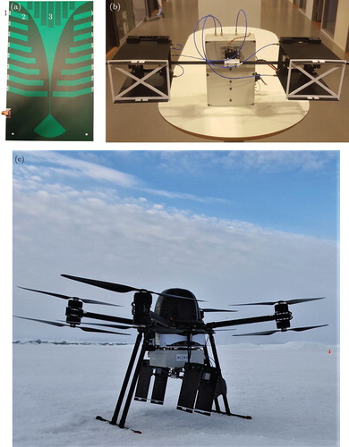
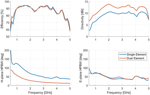
Figure 4. Simulated antenna parameters.

The spacing between the antennas was optimized through simulation. The ideal distance for a 0.7–4.5 GHz bandwidth was found to be about 11 cm.

Figure 3(b) shows the two sets of Vivaldi antennas mounted in a bistatic configuration with approximately 50 cm spacing between the pairs. The TX signal is distributed to the two Vivaldi antennas using a 2-way power splitter. The radar system has two RX inputs enabling a direct connection with each RX antenna. The antenna mounting is entirely 3D printed resulting in a lightweight, easy to manufacture and nearly electrically neutral part.

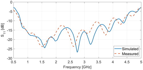
Simulations of the antenna array configuration was performed in CST microwave studio suite,⁴ and is shown in Figure 4. The simulations show approximately 3 dBi increased directivity across the frequency range, and a significant reduction in half power beam width (HPBW) in the H-plane beam compared to a single element antenna. The increase in directivity is similar to the directivity of a dipole in the H-plane. Simulations also show little change in the antenna efficiency and the same $S_{11}$ (Figure 5) if we assume ideal power splitting and that parasitic effects between the dual elements are negligible. Comparing the simulated and measured $S_{11}$ in Figure 5 shows a slight shift downwards in the band. This might be due to the dielectric effect of the antenna silkscreen not included in the simulation. Additionally, we have installed an RF amplifier (Minicircouts ZX60-83LN12+) that increased the nominal output power from −7 dBm to 17.3 dBm. These improvements are all motivated by increasing the penetration depth and effective observation range of the radar system.

Figure 5. Simulated and measured return loss for the modified Vivaldi antenna.

A servo-based antenna angle regulation mechanism was designed to enable measurements in slanted terrain as well as working to stabilize the antenna from UAV movement. The angle regulation mechanism can be set to keep a specific angle and use the UAV gyroscope to regulate that angle relative to the UAV movements; however, only along one axis. When performing surveys over flat terrain, the angle regulation mechanism points the antennas in nadir. Furthermore, the UAV has retractable feet minimizing clutter from the UAV air-frame.

Table 2 compares the dual Vivaldi antenna configuration with the single Vivaldi antenna configuration used on the previous iteration of the radar system. In addition to the dual configuration, the new Vivaldi antennas have inserted slits which effectively shifts the bandwidth of the antenna downwards. As seen in Table 2, the antenna bandwidth is also reduced by approximately 1.25 GHz resulting in approximately 1 cm degraded range resolution. However, the penetration depth for wet snow is almost doubled with this configuration.

Table 2. Comparison of single Vivaldi antenna and dual modified Vivaldi antenna.

Antenna configuration	Single	Dual with slits
Bandwidth	0.95–6 GHz	0.7–4.5 GHz
Penetration depth^a	9.7 m	18.2 m
Theoretical range resolution	2.97 cm	3.94 cm
Directivity at 2 GHz	10.5 dBi	13.9 dBi

^aCalculated at lowest frequency in bandwidth for snow with 1% liquid water content (LWC).

3.4. Other improvements

The radar sensor and radio modem have been modified with 3D printed enclosures to reduce weight. This modification results in a weight reduction of 75% compared to the original aluminum housings. The 3D printed enclosures were coated in conductive paint to provide RF shielding. Further, the Odroid XU4 can read the Mavlink data stream coming from the UAV autopilot and store relevant data such as altitude, heading, speed, and position, together with the pre-processed radar data.

Direct connection to the UAV batteries produces significant noise due to the high variation in current draw from the speed regulators. The power handling board allows the radar system to accept a direct connection to the batteries using power filtering and regulation to 12 and 5 volts. The radar system now accepts 12–48 V at the power input.

The 868 MHz radio modem generates a network link between the ground station PC and the single board computer onboard the UAV. This enables full control of the radar system while airborne, as well as monitoring of the status of the radar system such as temperature and analog-to-digital converter (ADC) levels. Additionally, when using a higher bandwidth modem (e.g. 2.4 GHz), real-time processing and live stream of the radar image is enabled.

4. Methods: software improvements

This section will briefly go through the processing steps of the radar data, before presenting a method on how to measure outside the unambiguous range with this kind of radar, as well as presenting a calibration procedure to remove the effect of varying altitude.

4.1. Radar data processing

With limited antenna isolation owing to UAV mounting restrictions, the main focus of the processing is to remove antenna cross-talk and improve signal to noise ratio (SNR). The first technique applied to the radar data is the match filter processing performed on each received A-scan by cross-correlating the received signal with a locally stored sequence matching the transmitted sequence. This cross-correlation is stored locally on the radar control computer.

The post-processing procedure involves subtracting a reference measurement, normally a measurement from a flight well above the unambiguous range of the radar, or subtracting the slow-time mean of the entire B-scan to only look at dynamics in the data.

The signal then undergoes an FFT Hanning-windowing procedure, Hilbert transform windowing and is finally interpolated to fit the range relative to the propagation velocity in the medium under investigation. In the case of snow, the distance to the air-snow interface is first measured by processing the radar data as if the intermediate propagation medium for the radar signal was air, which is then changed at the identified air-snow interface.

The detection of the first interface can be done automatically or manually, depending on the overall SNR in the data. If the data is very noisy (i.e. from high altitude measurements, say above 20 m), the automatic detection procedure has problems detecting the correct interface which often is visible to the human eye.

Additional image processing methods such as Wiener filtering is used to reduce speckle, and contrast stretching can be applied to increase the contrast in the image for ease of interpretation.

The pre-processed image will be influenced by the varying altitude of the UAV. When the UAV is in “altitude hold” mode, the altitude variation according to the laser altimeter (and the first reflection in the radar image) is approximately 40 cm. Therefore, it could be beneficial to rectify the image based on the laser altimeter. If altimetric data are available from the UAV-mounted laser altimeter, the air-snow interface reflection is corrected for the altitude variation. Figure 6 shows a segment of a transect before and after altitude correction. The top surface of the snowpack is treated as flat for the purpose of measuring snow depth. The shifting procedure is a circular shift at each A-scan according to the laser altitude taken at the closest timestamp.

Figure 6. Example radar image before and after altitude correction.

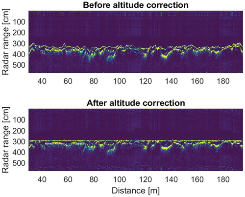
The processing steps of the altitude correction shown in Figure 6 can be listed as follows:

• Associate each A-scan with a laser altitude measurement using corresponding timestamps.

• Find closest index of laser altitude in radar range vector. Effectively converting laser altitude to radar range-bin position.

• Circularly shift each A-scan according to the converted laser altitude.

4.2. Measuring outside the unambiguous range

The output m-sequence signal generated from this sensor is a pseudo-random sequence that is correlated upon reception. One of the drawbacks of this waveform is that it is strictly periodic and cannot be delayed/range-gated to move the unambiguous range further down range. This results in an unambiguous range that depends on the sequence length and clock frequency (Equation (1) in [5]). The longer the sequence length, the longer the unambiguous range. However, the data size for each sequence will also increase and results in a reduction in measurement rate, if the processing power is not changed. For future “fixed-wing” UAV UWiBaSS applications, ground speed and altitude will increase significantly compared with multi-rotor UAV. Therefore, we need a method to increase the range of the radar system while keeping the measurement rate as high as possible.

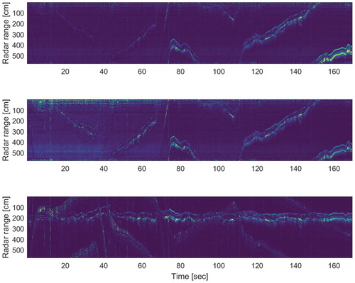
After reception, the received signal goes through a match filter process. If we consider the case of a single target moving down range from the radar, when the target moves to the end of the unambiguous range, it becomes wrapped around to the beginning of the radar range. We e.g. have a radar system with 10 m unambiguous range and a target at 12 m; in theory, the target should appear at 2 m after the match filter procedure. This is due to the inherent cyclic property of convolution using the discrete Fourier transform (DFT) in match filter processing, and can not be avoided. For drone-mounted GPR, where there usually is air between the antennas and the target (ground), we can assume that in most cases the air will appear as a homogeneous medium with little attenuation and marginal clutter. In this situation, we can perform measurements with the radar system while the target is outside the unambiguous range. This idea was tested in a field campaign on Svalbard 2019, where Figures 7 and 9 show that the radar system is able to measure the snow depth at altitudes far beyond the unambiguous range. We also observe that the received power decreases according to the radar equation (Figure 8), which will eventually limit the range of the radar system due to a smaller SNR with distance.

Figure 7. Example showing radar image and UAV altitude with the UAV mostly flying outside the unambiguous range, and entering the ambiguous range at approximately 150 s.

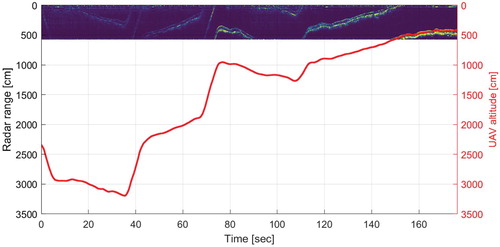
Figure 8. Returned power compared to the theoretical returned power according to the radar equation. Data was collected with a drone-mounted radar with a max unambiguous range of 5.7 m.

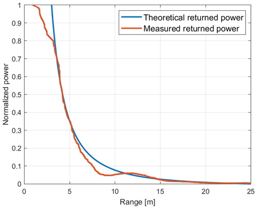
Figure 9. The same data as in Figure 7, before any correction (top) after altitude dependent power calibration (middle) and finally after the shifting procedure (bottom).

We could define a window; “Ambiguity window” in which our target should be contained such that it does not wrap around to the next window. As long as the path to the target is not obstructed, little or no clutter will be present. For the UWiBaSS the 3 first windows are defined in Table 3.

Table 3. Ambiguity windows.

Window number	Start of window	End of window
1	0 m	5.7 m
2	5.7 m	11.4 m
3	11.4 m	17.1 m

To avoid ambiguities in the measurements, the radar system is used in conjunction with a laser rangefinder. The rangefinder does not need high resolution for the purpose of identifying which window our target is within. Nevertheless, high resolution is needed for the altitude correction and the calibration procedure presented later in this paper.

The advantage of measuring outside the unambiguous range is that we can use sensors with short-windows which benefit from high measurement rate and less unnecessary data (e.g. data used to describe propagation in the air). However, one of the drawbacks of using a shorter shift registry for the m-sequence is that this raises the noise floor [5]. Additionally, if the target length (in this case, the snow depth) is longer than the unambiguous range, the measured profile will overlap, thus complicating the interpretation.

Other studies show similar results for CW radars. Albanese and Klein [40] have shown that using two code clocks can extend the unambiguous range. Zhang et al. [41] demonstrated a similar solution to range ambiguity using FMCW signals in combination with two-tone CW signals to obtain high precision range measurements with SDR.

The major drawback of using CW radars beyond the unambiguous range are that one can not increase the output power indefinitely. In a bistatic CW radar, the RX antenna is always receiving and if the TX power is too high, the receiver electronics can be saturated or even blown by the antenna crosstalk. This can, in principle, be solved by using range gated radar systems [10].

Figure 7 show an example data-set chosen for high variations on altitude. This case can be considered extreme since the UAV normally maintains a somewhat stable altitude (e.g. Figure 6) during data collection. However, this example was chosen to illustrate how the processing method works.

From Figures 7 and 8, we can construct a calibration procedure that shifts and calibrates each A-scan according to the laser altimeter. The shifting procedure is the same method as shown in Figure 6. Calibration involves multiplying each slowtime vector (corresponding to a laser altitude) with the range dependence from the radar equation. In this case, we are using the special variant of the radar equation for flat surfaces [42]. The calibrated pixel value in terms of power $n_c$ becomes: (6) $n_c=n(4\pi {)}^2(2R_{alt}{)}^2,$(6) where n is the non-calibrated pixel value in terms of power and $R_{alt}$ is the radar altitude. This calibration procedure results in pixel values that are independent of altitude and mostly depend on the changes in dielectric constant at different media interfaces.

Figure 9 show an example of how to process the radar data such that we can measure outside the unambiguous range. Notice in the bottom image in Figure 9 that the crosstalk varies as the inverse of the radar altitude. Improved crosstalk rejection will mitigate this. Also, notice that the rectification is far from perfect regarding the air-snow interface. This is due to the different mounting positions of the UWiBaSS and the laser altimeter on the UAV resulting in different responses to small angles when the UAV tilts. The most apparent variation occurs when the UAV has rapid changes in altitude, which should be avoided in normal data collection scenarios. Additionally, inaccuracies in the laser altimeter play a small part. Nevertheless, this result can be used in further analysis and image improvement.

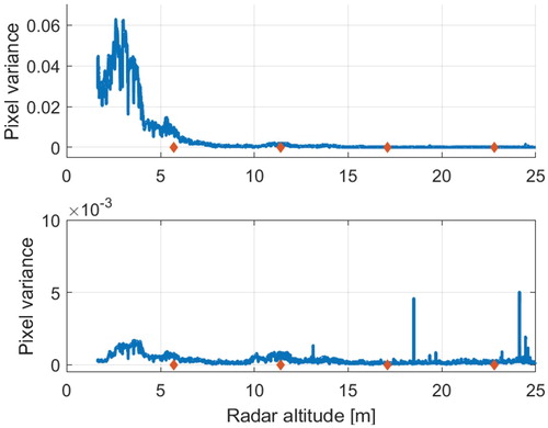
A comparison of the pixel variance before and after the calibration procedure is shown in Figure 10, where the variance stays significantly more constant in the calibrated image. However, a slight increase in variance is shown as altitude rises. This is because we are introducing more noise to the image with this calibration. With this calibration procedure, the variation in the received radar signal due to the radar altitude is almost removed. This procedure could be used to estimate the density, and possibly the dielectric constant for dry snow if we can ignore the imaginary part of the dielectric constant.

Figure 10. Pixel variance of the un-calibrated (top) and range calibrated (bottom) radar image. Ambiguity windows are marked with red diamonds.

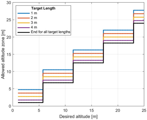
The antenna crosstalk is not that trivial to remove when facing UAV mounted radar. This is due to both variable radio interference influencing the entire image, but mostly due to vibrations and moving parts close to the antennas (such as UAV landing gear). This leads us to altitude windows we could recommend the pilot to stay inside to keep the cross talk in a different image region than the target. Due to moving landing gear, or other small moving parts relatively close to the antennas, we can, in general, say that we should have the target at least 1 m down range from the cross talk, regardless of what ambiguity window we are in. We must also consider the approximate depth of the target to avoid having the target move into the next window. From this general rule, we can create regions of preferred altitude a for the pilot to stay inside. (7) $a=[R_u(W-1)+1]R_{u}W-T,$(7) and (8) $W=floor\left(\frac{R_{alt}}{R_u}\right)+1,$(8) where $R_u$ is the unambiguous range of the radar, W is the “ambiguity window” number, T is the expected length of the target, floor is a function that returns the greatest integer less than or equal to the input and $R_{alt}$ is the approximate altitude the UAV is to fly in (e.g. 5, 10 or 15 m). This rule is visualized in Figure 11 for a radar system with 5.75 m unambiguous range and target lengths (i.e. snow depths) of 1,2,3 and 4 m. From this figure, we can see that the longer a target is, the shorter is the preferred range for the UAV to fly in.

Figure 11. Chart of preferred zones of altitude given different target lengths. This is calculated for a radar system with 5.75 m unambigous range.

5. Field results

In this section, we present results from a field campaign conducted in 2019 on Svalbard. We make comparisons against both in situ measured depth as well as in situ stratigraphy.

During March 2019 we conducted a 7-day campaign in the area around Longyearbyen – Svalbard. This campaign focused on snow depth measurements over approximately $100\mathrm{m}\times 100\mathrm{m}$ grids. The grids were scanned with the UWiBaSS mounted on the Cryocopter FOX UAV and manually measured using the Snow-Hydro GPS snow depth probe,⁵ and in “High res. 1” and “High res. 2” with standard avalanche probe and handheld GPS (see Figure 12). This field campaign was carried out as a part of the Svalbard integrated arctic earth observing system (SIOS) project to monitor snow cover on Svalbard.

Figure 12. Map of SIOS field locations. Sites visited on the current campaign is marked in red.

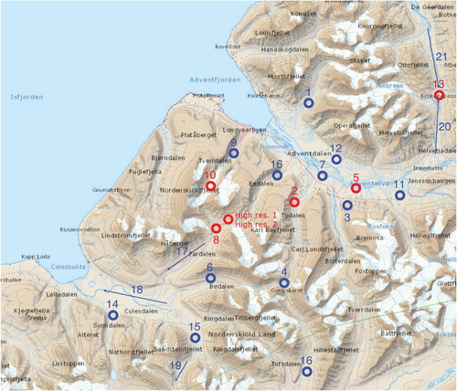
21 field locations were defined to do recurring measurements over a 5 year period. Due to time limitations and avalanche safety restrictions though, only some of the sites were visited during the 2019 campaign and these are marked red in Figure 12. On each site, a $100\mathrm{m}\times 100\mathrm{m}$ grid with 10 m spacing between transects was selected for snow depth survey using the UWiBaSS mounted on UAV and also using GPS snow probe.

The UWiBaSS data can be displayed as a 1D (A-scan) snow profile as seen in Figure 14 or as a 2D cross-section (B-scan) of the snowpack as seen in Figure 13. Additionally, the depth measurements obtained with the UWiBaSS can be combined with the GPS data from the UAV to make snow depth maps that can be overlaid onto maps, as seen in Figure 15.

Figure 13. B-scan radar image from site “High res. 1”, with interpreted radar snow depth compared with in situ snow depth. The radar measurement is a 100 m transect with 38 manual measurements over nearly 80 m. All data points are geo-referenced.

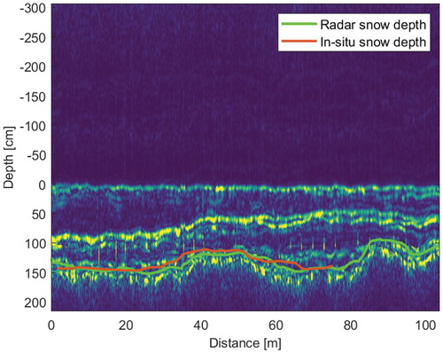
Figure 14. A-scan radar responses in red (150 slow time averages), compared to in situ stratigraphy in blue, assessed using the “hand test” [43] shown with the top x-axis. (a) Site 4 and (b) Site 8.

Figure 15. Georeferenced snow depth from site 2, measured with drone mounted radar (a) and GPS snow probe (b). $C=0.67\pm 0.01$ and root-mean-square error (RMSE) $=5.9$ cm. (a) Radar snow depth and (b) In situ snow depth.

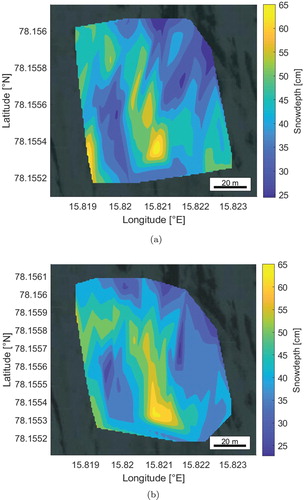
Figure 13 shows the B-scan radar image from a 100 m transect with nearly 80 m of in situ depth measurements. The data has been georeferenced and plotted together. The radar measurements were performed at approximately 8 m altitude above the snow cover. Hence, the original data before laser range correction had the snowpack overlapping two “ambiguity zones”. The crosstalk zone is noticeable as a thin line of noise at approximately 100 cm in Figure 13.

Figure 14 shows in situ stratigraphy compared with the radar response from an area close to the snow pit. The in situ stratigraphy was collected using the “hand test” for assessing snow hardness [43]. The top peak in the radar response is a combination of the air-snow interface and internal variations at the top of the snowpack. The middle peaks correlate with the distinct internal layers in the snowpack. The bottom also gives a distinct response in the radar image, while the in situ profile does not mark that transition.

In Figure 13, we can identify the top and bottom interfaces automatically or manually. This depth data are then referenced to the range vector that is calculated based on the propagation velocity for each medium. The depth data from each B-scan are then associated with a GPS coordinate and can be displayed as a contour map on top of existing maps. This can be useful for estimations of total snow volume or finding areas with varying snow cover.

Figure 15 shows a $100\mathrm{m}\times 100\mathrm{m}$ grid of georeferenced depth measurements by the radar and compared to in situ depth. The depth estimations are interpolated into a surface and overlaid on a map where some correlation with the features in the surrounding image is seen (e.g. Rocky parts in the map correlates to areas with low snow depth). The depth measurements in Figure 15 are correlated with in situ depth in Figure 16 marked in blue.

Figure 16. In-situ snow depth vs. radar snow depth for all sites. Spatial correlation: $C=0.97\pm 0.01$ and RMSE $=10.6$ cm.

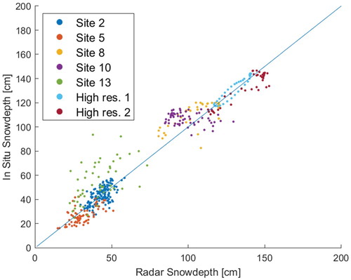
Finally, Figure 16 shows combined spatial snow depth correlations for all sites visited, where each in situ depth measurement is correlated to its closest radar depth measurement based on the GPS positions of the GPS probe and UAV. In “High res.” 1 and 2 we used manual depth probes for the depth measurements, while in the other sites we used the GPS probe. The max depth for the GPS probe is 120 cm, hence, radar snow depth measurements were thresholded at 120 cm for the sites where the GPS probe was used. However, for the “High res.” 1 and 2 transects, a standard avalanche probe was used, and coincidentally the snow depth was up to 153 cm at those sites.

6. Discussion

One of the main challenges of snow measurements with radar is sufficient penetration depth. The latest iteration of the antennas for the UWiBaSS is using different methods to obtain acceptable penetration depth for snow sensing tasks. More power is concentrated on a smaller footprint by increasing antenna directivity and transmitted power. Additionally, by shifting the radar system bandwidth down from 0.95–6 GHz to 0.7–4.5 GHz, penetration depth in the snow has been increased further.

Furthermore, a range calibration procedure removes the influence of distance to the target. When the range variability is removed, density will mainly govern the amount of back-scattered power (for dry snow). Grain size and surface roughness also influence the returned power, however, for the frequency domain of the UWiBaSS, we might be able to ignore those parameters for coarse density estimation. Figure 9 shows how the calibration procedure alters the image. Notice the weak returns at the start of the image become more clear, but at the expense of more noise.

Results from the Svalbard campaign further confirm that UWiBaSS is a capable snow measurement system, and the improved antenna system significantly improved the platform stability as well as the dynamic range in the received data.

The antenna system should be upgraded to a 2 axis angle adjustment mechanism to further stabilize the antennas from UAV movement. However, stabilization in one axis significantly improved the overall stability of the antennas.

The UAV with antennas was tested in winds up to 15 m/s without any significant issues regarding flight or influence from the antennas in the wind. Additionally, the UWiBaSS was tested at the maximum speed of the UAV, approximately 21 m/s, with no noticeable degradation due to vibration. However, with fewer measurements to average over for each position when the UAV speed increases, the noise level is expected to increase.

A comparison between the A-scan radar response and the in situ snow stratigraphy in Figure 14 shows an agreement regarding the layers contained inside the snowpack. One should note that the radar signal have strong reflections at the ground surface which is not considered in the in situ case. Additionally, the transition from air-to-snow also gives a strong response not taken into account in the in situ stratigraphy. Looking at Figure 13, the stratigraphy is dynamic even at sub 10 m distances. Hence, ideally, the radar measurement should be taken as close as possible to the in situ snow pit. In the case of Figure 14 the in situ profile was taken approximately 2 m from the radar transect.

Figure 15 shows good agreement between the radar and in situ depth mapping. As seen in Figure 16, similar spatial correlations were found for the remaining sites.

Comparing the radar and in situ depth yields a correlation coefficient of $0.97\pm 0.01$ and RMSE of 10.6 cm, which are amongst the highest reported correlations compared to other studies in the literature [6–8,11]. The correlation given by the depth measured by the GPS probe (e.g. Figure 15) compared to the high resolution transects (e.g. Figure 13) is significantly lower as seen in Figure 16. That leads us to believe that other factors such as GPS accuracy and the low resolution in the in situ measurements also influence the correlation coefficient. This is mainly due to the high variability of the snow depth caused by the dynamic terrain below, which is not captured by the low resolution in situ measurements. The RMSE is reduced to 5.8 cm if we only consider the sites where the manual snow probe was used (High res. 1 and 2). These measurements were also the deepest depth measurements with values up to 153 cm.

7. Conclusion

In this paper, we have presented improvements to the UWiBaSS radar system. This includes new and improved antennas and signal processing techniques.

The improved directivity of the new Vivaldi array improves the ability to penetrate snow and to measure with a smaller antenna footprint at higher flight altitudes.

Using a calibration procedure to compensate for the altitude in the radar data allows for the extraction of other pieces of information from the back-scattered signal. Potentially, one could find a relation between back-scattered power and snow density. This will be investigated in future work.

A major challenge in the verification of such a system is the high variability in the snowpack, which is detected by the radar system, but not always by the in situ measurements due to the coarse spacing of manual measurement points. This is evident when comparing the correlations gained from the high resolution transects with the more coarsely spaced measurements performed with the GPS probe.

The system could be used to accurately estimate total snow volume, mass or snow water equivalent (SWE) using local density measurements. Future work includes investigating methods to extract the dielectric constant from snow data in order to establish the snow water equivalent by radar only. Additionally, the radar system will be mounted on a fixed-wing UAV to extend area coverage. For this application, the method to perform measurements outside the unambiguous range will be useful.

Disclosure statement

No potential conflict of interest was reported by the author(s).

Additional information

Funding

This work was supported by the Research Council of Norway under the project Svalbard Integrated Arctic Earth Observing System (SIOS) – Infrastructure development of the Norwegian node (Grant No. 269927); and the Centre for Integrated Remote Sensing and Forecasting for Arctic Operations (CIRFA) partners (Grant No. 237906); and NORCE Norwegian Research Centre (Grant No. 261786); Norges Forskningsråd.

Notes on contributors

Rolf Ole R. Jenssen

Rolf Ole Rydeng Jenssen received the B.Sc. degree in automation and the M.Sc. degree in applied physics and mathematics, with a focus on snow stratigraphy measurements with ultra-wideband radar, from the University of Tromsø-Arctic University of Norway, Tromsø, Norway, in 2014 and 2016, respectively. Since 2017, he has been a Ph.D. Fellow with the Centre for Integrated Remote Sensing and Forecasting for Arctic Operations (CIRFA), Tromsø, where he is involved in unmanned aerial vehicle remote sensing for Arctic applications such as monitoring of snow and sea ice conditions.

Svein Jacobsen

Svein Jacobsen (M'02–SM'07) was born in Norway in 1958. He received the B.Sc. and M.Sc. degrees and the Ph.D. degree in microwave sensing of the ocean surface from the University of Tromsø, Tromsø, Norway, in 1983, 1985, and 1988, respectively. From 1985 to 1986, he was a Researcher with Information Control Ltd., where he was involved in space-borne observation platforms for the earth- probing satellite ERS-1. From 1989 to 1992, he was a Research Scientist with the Norwegian Research Council for Science and Humanities, where he was involved in nonlinear mapping of the ocean surface by means of synthetic aperture imaging radar. From 2000 to 2001, he did a research sabbatical at the University of California at San Francisco, San Francisco, CA, USA, where he investigated the use of multiband microwave radiometry for temperature measurement in the human body. Since 2001, he has been a Professor of electrical engineering with the Department of Physics and Technology, University of Tromsø-The Arctic University of Norway, Tromsø. His current research interests include thermal medicine, development of active and passive microwave systems, applicators for diagnostic and therapeutic applications in the human body, development of miniature unmanned aerial vehicle-mounted ultra-wideband radars for various remote sensing applications including snowpack stratigraphy for hardness investigation and weak layer detection.

Notes

1 Visit the ILMsens website at https://www.ilmsens.com/products/m-explore/

2 For more information about “Here+” RTK GPS visit: http://ardupilot.org/copter/docs/common-here-plus-gps.html

3 For more information about SF11 visit: https://lightware.co.za/products/sf11-c-120-m

4 For more information about CST visit: https://www.3ds.com/products-services/simulia/products/cst-studio-suite/

5 For more information about the GPS snow depth probe, visit: http://www.snowhydro.com/products/column2.html

References

- Dierking W. Mapping of different sea ice regimes using images from Sentinel-1 and ALOS synthetic aperture radar. IEEE Trans Geosci Remote Sens. 2010;48(3):1045–1058. doi: 10.1109/TGRS.2009.2031806
- Mahoney A, Eicken H, Graves A. Landfast sea ice extent and variability in the Alaskan Arctic derived from SAR imagery. In: 2004 IEEE International Geoscience and Remote Sensing Symposium, 2004. IGARSS'04. Proceedings. Vol. 3. IEEE; 2004. p. 2146–2149.
- Farrell SL, Kurtz N, Connor LN, et al. A first assessment of IceBridge snow and ice thickness data over Arctic sea ice. IEEE Trans Geosci Remote Sens. 2012;50(6):2098–2111. doi: 10.1109/TGRS.2011.2170843
- Tiuri M, Sihvola A, Nyfors E, et al. The complex dielectric constant of snow at microwave frequencies. IEEE J Oceanic Eng. 1984;9(5):377–382. doi: 10.1109/JOE.1984.1145645
- Jenssen ROR, Eckerstorfer M, Jacobsen S. Drone-mounted ultrawideband radar for retrieval of snowpack properties. IEEE Trans Instrum Meas. 2020;69(1):221–230. doi: 10.1109/TIM.2019.2893043
- Marshall HP, Schneebeli M, Koh G. Snow stratigraphy measurements with high-frequency FMCW radar: comparison with snow micro-penetrometer. Cold Reg Sci Technol. 2007;47(1–2 Spec. Iss.):108–117. doi: 10.1016/j.coldregions.2006.08.008
- Singh KK, Datt P, Sharma V, et al. Snow depth and snow layer interface estimation using ground penetrating radar. Curr Sci. 2011;100(10):1532–1539.
- Yankielun N, Rosenthal W, Davis RE. Alpine snow depth measurements from aerial FMCW radar. Cold Reg Sci Technol. 2004;40(1–2):123–134. doi: 10.1016/j.coldregions.2004.06.005
- Kim Y, Reck TJ, Alonso-Delpino M, et al. A Ku-band CMOS FMCW radar transceiver for snowpack remote sensing. IEEE Trans Microw Theory Tech. 2018;66(5):2480–2494. doi: 10.1109/TMTT.2018.2799866
- Øyan MJ, Hamran SE, Hanssen L, et al. Ultrawideband gated step frequency ground-penetrating radar. IEEE Trans Geosci Remote Sens. 2012;50(1):212–220. doi: 10.1109/TGRS.2011.2160069
- Yan JB, Gomez-Garcia Alvestegui D, McDaniel JW, et al. Ultrawideband FMCW radar for airborne measurements of snow over sea ice and land. IEEE Trans Geosci Remote Sens. 2017;55(2):834–843. doi: 10.1109/TGRS.2016.2616134
- Kwok R, Panzer B, Leuschen C, et al. Airborne surveys of snow depth over Arctic sea ice. J Geophys Res Oceans. 2011;116(11):1–16.
- Rodriguez-Morales F, Gogineni S, Leuschen CJ, et al. Advanced multifrequency radar instrumentation for polar research. IEEE Trans Geosci Remote Sens. 2014;52(5):2824–2842. doi: 10.1109/TGRS.2013.2266415
- Tan A, Eccleston K, Platt I. The design of a UAV mounted snow depth radar results of measurements on Antarctic sea ice. 2017 IEEE Conference on Antenna Measurements & Applications (Cama), Tsukuba, Japan; 2017. p. 316–319.
- Li CJ, Ling H. High-resolution, downward-looking radar imaging using a small consumer drone. In: 2016 IEEE International Symposium on Antennas and Propagation (APSURSI), Fajardo, Puerto Rico; Vol. 2; 2016. p. 2037–2038.
- Li CJ, Ling H. Synthetic aperture radar imaging using a small consumer drone. IEEE International Symposium on Antennas and Propagation; Vancouver, Canada; Vol. 10(d); 2015. p. 4–5.
- Tarchi D, Guglieri G, Vespe M. Mini-radar system for flying platforms. In: 4th IEEE International Workshop on Metrology for AeroSpace, MetroAeroSpace 2017 – Proceedings, Padua, Italy; 2017. p. 40–44.
- Lort M, Aguasca A, López-Martínez C, et al. Initial evaluation of SAR capabilities in UAV multicopter platforms. IEEE J Sel Top Appl Earth Obs Remote Sen. 2018;11(1):127–140. doi: 10.1109/JSTARS.2017.2752418
- Šipoš D, Peter P, Gleich D. On drone ground penetrating radar for landmine detection. In: 2017 First International Conference on Landmine: Detection, Clearance and Legislations (LDCL), Beirut, Lebanon; 2017. p. 7–10.
- Yarleque MA, Alvarez S, Martinez HJ. FMCW GPR radar mounted in a mini-UAV for archaeological applications: First analytical and measurement results. In: 2017 International Conference on Electromagnetics in Advanced Applications (ICEAA), Verona, Italy; Vol. 9. IEEE; 2017. p. 1646–1648.
- Fitter JF, Mccallum AB, Leon JP. Development of an unmanned aircraft mounted software defined ground penetrating radar. Geotechnical and Geophysical Site Characterisation, Australian Geomechanics Society; Vol. 5; 2016. p. 957–962.
- Burr R, Schartel M, Mayer W. Uav-Based Polarimetric Synthetic Aperture Radar for Mine Detection. IGARSS 2019–2019. IEEE International Geoscience and Remote Sensing Symposium, Yokohama, Japan; 2019. p. 9208–9211.
- Rodriguez-Vaqueiro Y, Vazquez-Cabo J, Gonzalez-Valdes B. Array of antennas for a GPR system onboard a UAV. 2019 IEEE International Symposium on Antennas and Propagation and USNC-URSI Radio Science Meeting, APSURSI 2019 – Proceedings, Atlanta, GA, USA; 2019. p. 821–822.
- Drinkwater MR, Crocker GB. Modelling changes in the dielectric and scattering properties of young snow-covered sea ice at GHz fequencies. J Glaciol. 1988;34(118):274–282. doi: 10.1017/S0022143000007012
- Daniels D. Ground penetrating radar. Vol. 1. London, UK: The Institution of Engineering and Technology; 2013.
- Nandan V, Geldsetzer T, Yackel JJ, et al. Multifrequency microwave backscatter from a highly saline snow cover on smooth first-year sea ice: first-order theoretical modeling. IEEE Trans Geosci Remote Sens. 2017;55(4):2177–2190. doi: 10.1109/TGRS.2016.2638323
- Ulaby FT, Abdelrazik M, Stiles WH. Snowcover influence on backscattering from terrain. IEEE Trans Geosci Remote Sens. 1984;GE-22(2):126–133. doi: 10.1109/TGRS.1984.350604
- Drinkwater MR. LIMEX '87 ice surface characteristics: implications for C-band SAR backscatter signatures. IEEE Trans Geosci Remote Sens. 1989;27(5):501–513. doi: 10.1109/TGRS.1989.35933
- Hufford GA. A model for the complex permittivity of ice at frequencies below 1 THz. Int J Infrared Millimeter Waves. 1991;12(7):677–682. doi: 10.1007/BF01008898
- Matzler C, Wegmuller U. Dielectric properties of freshwater ice at microwave frequencies. J Phys D Appl Phys. 1987;20(12):1623–1630. doi: 10.1088/0022-3727/20/12/013
- Hallikainen MT, Ulaby FT, Abdelrazik M. Dielectric properties of snow in the 3–37 GHz range. IEEE Trans Antennas Propag. 1986;AP-34(11):1329–1340. doi: 10.1109/TAP.1986.1143757
- Tsang L, Kong JA. Scattering of electromagnetic waves from random media with multiple scattering included. J Math Phys. 1982;23(6):1213–1222. doi: 10.1063/1.525453
- Huining W, Pulliainen JT, Hallikainen MT. Effective permittivity of dry snow in the 18–90 GHz range. J Electromagn Waves Appl. 1999;13(10):1393–1394. doi: 10.1163/156939399X00727
- Mätzler C. Relation between grain size and correlation length of snow. American Geophysical Union Fall Meeting, San Francisco, California; Vol. 48; 2002. p. 1–4.
- Onstott RG, Shuchman RA. SAR measurements of sea ice. SAR Marine User's Manual; Vol. 3; 2004. p. 81–115.
- Richards MA. Fundamentals of radar signal processing. New York: McGraw-Hill Professional; 2015.
- Jenssen ROR. Snow stratigraphy measurements with UWB radar; 2016. Available from: http://hdl.handle.net/10037/11117.
- Kim SW, Choi DY. Implementation of rectangular slit-inserted ultra-wideband tapered slot antenna. SpringerPlus. 2016 Aug;5(1):1387. doi: 10.1186/s40064-016-3033-4
- Avdushin AS, Ashikhmin AV, Negrobov VV, et al. Vivaldi antenna with printed lens in aperture. Microw Opt Technol Lett. 2014 Feb;56(2):369–371. doi: 10.1002/mop.28120
- Albanese D, Klein A. Pseudo-random code waveform design for CW radar. IEEE Trans Aerosp Electron Syst. 1979;AES-15:67–75. doi: 10.1109/TAES.1979.308797
- Zhang H, Li L, Wu K. Software-defined six-port radar technique for precision range measurements. IEEE Sens J. 2008;8(10):1745–1751. doi: 10.1109/JSEN.2008.2003304
- Haynes MS. Surface and subsurface radar equations for radar sounders. Annals of Glaciology. 2020;16:1–8. doi: 10.1017/aog.2020.16
- Greene E, Birkeland K, Elder K. Observation guidelines for avalanche programs in the United States. Bozeman (MT): American Avalanche Association; 2016.