Application of cylindrical IE-GSTC to physical metasurfaces

Abstract

The cylindrical Integral Equation -- Generalized Sheet Transition Condition (IE-GSTC) is validated by applying it to physical metasurfaces, i.e. metasurfaces defined by material properties and dimensions rather than by susceptibility tensor components. The previously reported IE-GSTC, which was formulated for zero thickness GSTC discontinuities, is extended to handle the finite thickness of physical metasurfaces. A simple analytical approach is used to extract the bianisotropic susceptibility tensor of concentric, multilayered, magneto-dielectric shells. Plane wave scattering by a physical metasurface constructed of four segments of multilayered, magneto-dielectric metasurface scatterers is used as an example problem to validate cylindrical IE-GSTC. A second example considers an opening on the cylindrical metasurface, confirming IE-GSTC can handle metasurfaces with openings. Third example is that of plane wave scattering by an eight segment metasurface. Good agreement is obtained between IE-GSTC results and full wave simulation results for all the cases. The paper concludes with a novel technique to handle PEC segments embedded in a cylindrical metasurface.

Keywords:

• Metasurface
• cylindrical
• MoM
• GSTC
• bianisotropic

1. Introduction

Metasurfaces, the 2D version of volumetric metamaterials, have provided unprecedented ability in the control and manipulation of electromagnetic waves. In comparison to metamaterials, metasurfaces are easier to fabricate, less bulky and have lower loss. Metasurfaces are electrically thin surfaces constructed using subwavelength particles called metaatoms. By using engineered particles, metasurfaces can transform the phase, amplitude, polarization and propagation direction of the incident wave. Several review articles and books exist on the analysis, design, modeling and applications of planar metasurfaces [1–4]. Due to its deeply subwavelength thickness, physical metasurfaces can be abstracted as an infinitesimally thin layer of electric and magnetic surface polarization densities. Metasurfaces achieve their functionality by creating a spatial electromagnetic discontinuity. Mathematically, the discontinuity can be expressed by Generalized Sheet Transition Conditions (GSTCs) which relate the electric and magnetic field discontinuities to the electric and magnetic surface polarization densities [5,6]. The surface polarization densities are related to the average of the fields on either side of the GSTC surface through the bianisotropic susceptibility tensor model [7]. It should be noted that even though physical metasurfaces have a finite subwavelength thickness, GSTCs which assume zero metasurface thickness are a very good approximation to such physical metasurfaces, i.e. the scattered field due to the physical metasurface approximates the field scattered by GSTC interface conditions.

GSTCs in combination with the bianisotropic susceptibility tensor model can be effectively used to simulate thin electromagnetic surfaces. Previous works in this approach include the application of Finite Difference Frequency Domain (FDFD) method [8] and Finite Element Method (FEM) [9] to the modeling of planar GSTCs. Even though most of the metasurfaces reported to date are planar, other canonical shapes such as cylindrical metasurfaces [10–13] and spherical metasurfaces [14,15] are now being studied. Applications of conformal metasurfaces include illusion transformation [13], cloaking [12], camouflaging [16], high-gain antennas [17] and so on. GSTC bianisotropic susceptibility tensor model had been previously used for conformal metasurfaces. An Integral Equation -- Method of Moment (IE-MoM) approach was applied to circular cylindrical metasurfaces in [10]. This was extended to cylindrical metasurfaces of arbitrary cross-section in [11]. Conformal transformation was used to synthesize surface electromagnetic tensor quantities for non-circular cylindrical metasurface in [18]. In [19], a digital signal processing based method is outlined for analysis and synthesis of cylindrical, bianisotropic metasurfaces. In [20], an inverse source technique was used to synthesize surface susceptibility tensor components of metasurfaces of arbitrary shape. The work addressed metasurfaces capable of generating radiation patterns with specified half-power beamwidth, nulls, polarization etc. Recently, asymptotic methods (GO, GTD) were applied to electrically large metasurfaces [21]. A wave matrix approach for analysis and synthesis of cascaded cylindrical metasurfaces was reported in [22]. Even though mathematically rigorous, none of these works [10–12,14,20,21,23–25] have used physical metasurfaces.

One of the goals of this paper is to move from the bianisotropic susceptibility tensor based conformal GSTC surface models used in [10–12,14,20,21,23–25] to physical metasurfaces formed by curved metasurface scattering particles. In this work, validity of the cylindrical GSTC [10] is confirmed by comparing the scattering due to a cylindrical, physical metasurface to scattering by a corresponding GSTC contour. Scattering by a cylindrical GSTC contour was obtained by a slightly modified version of IE-GSTC formulation in [10]. The modification incorporates the finite thickness of physical metasurfaces. This modification is important to get accurate results for IE-GSTCs [10,11,24] when compared to physical metasurface scattering.

The organization of the paper is as follows. Section 2 extends the IE-MoM in [10] to handle a physical metasurface with non-zero thickness. The contents of this section closely follow [10]. Only the significant differences are explained. Section 3 details the susceptibility tensor extraction of cylindrical, concentric, magneto-dielectric shell using an analytical approach. Section 4 provides two examples. The metasurfaces in the two examples are constructed using metasurface particles which are part of the shell structure in Section 3. The second example has an opening which can be modeled using the IE-GSTC formulation, but with reduced accuracy. The IE-GSTC, using susceptibility tensors extracted using the method in Section 3, is used to simulate the scattering problem, with the results compared with a full wave simulation of the physical metasurface. The final section, Section 5 provides a detailed formulation for handling PEC segments in cylindrical metasurfaces with one numerical validation example.

2. IE-MoM for finite thickness cylindrical metasurface

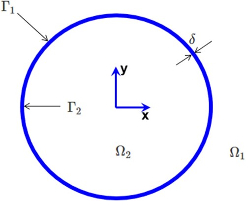
The IE-MoM described in [10] was limited to a cylindrical GSTC contour of zero thickness whose surface polarization densities are related to electric and magnetic fields on either side of the metasurface by the bianisotropic susceptibility tensor model. That formulation needs to be slightly extended to include the non-zero thickness of a physical metasurface. Instead of using a single contour for calculating MoM coefficients and integration of surface fields, two contours (one external and other internal to the metasurface) are used. The problem geometry is shown in Figure 1. Throughout this paper, there is no variation of material properties or excitation along the z axis. The inner contour is ${\mathrm{\Gamma }}_2$ and the outer contour is ${\mathrm{\Gamma }}_1$, separated by the metasurface thickness δ.

Figure 1. Finite thickness cylindical metasurface.

This is a figure of cylindrical metasurface. It is a circle with z-axis perpendicular to the figure, the x-axis is towards right. The inner region of circle is denoted by omega subscript 2 and outer region of the circle is denoted by omega subscript 1. The inner contour is denoted by gamma subscript 2 and outer contour is denoted by gamma subscript 1.

In this section, the extension of the formulation in [10] is outlined. A clear understanding of [10] is required to understand this section. The variables and notations follow [10]. The 2D IEs for TM polarization given in Equation (6) of [10] are modified to (1a) $\begin{array}{rl}& E_{z1}^{\mathrm{inc}}(\overline{\rho })+{\oint }_{{\mathrm{\Gamma }}_1}[E_{z1}({\overline{\rho }}_1^{\mathrm{\prime }})\frac{\mathrm{\partial }{G}_0(\overline{\rho };{\overline{\rho }}_1^{\mathrm{\prime }})}{\mathrm{\partial }{n}^{\mathrm{\prime }}}-j\omega {\mu }_0{H}_{\varphi 1}({\overline{\rho }}_1^{\mathrm{\prime }})G_0(\overline{\rho };{\overline{\rho }}_1^{\mathrm{\prime }})]\mathrm{d}{\mathrm{\Gamma }}_1^{\mathrm{\prime }}\\ & =\{\begin{array}{ll}{E}_{z1}(\overline{\rho });& \overline{\rho }\in {\mathrm{\Omega }}_1\\ 0.5E_{z1}(\overline{\rho });& \overline{\rho }\in {\mathrm{\Gamma }}_1\\ 0;& \overline{\rho }\in {\mathrm{\Omega }}_2\end{array}\end{array}$(1a) (1b) $\begin{array}{rl}& E_{z2}^{\mathrm{inc}}(\overline{\rho })-{\oint }_{{\mathrm{\Gamma }}_2}[E_{z2}({\overline{\rho }}_2^{\mathrm{\prime }})\frac{\mathrm{\partial }{G}_0(\overline{\rho };{\overline{\rho }}_2^{\mathrm{\prime }})}{\mathrm{\partial }{n}^{\mathrm{\prime }}}-j\omega {\mu }_0{H}_{\varphi 2}({\overline{\rho }}_2^{\mathrm{\prime }})G_0(\overline{\rho };{\overline{\rho }}_2^{\mathrm{\prime }})]\mathrm{d}{\mathrm{\Gamma }}_2^{\mathrm{\prime }}\\ & =\{\begin{array}{ll}0;& \overline{\rho }\in {\mathrm{\Omega }}_1\\ 0.5E_{z2}(\overline{\rho });& \overline{\rho }\in {\mathrm{\Gamma }}_2\\ E_{z2}(\overline{\rho });& \overline{\rho }\in {\mathrm{\Omega }}_2\end{array}\end{array}$(1b) where ${\overline{\rho }}_1^{\mathrm{\prime }}$ and ${\overline{\rho }}_2^{\mathrm{\prime }}$ denote contour integration position variables along ${\mathrm{\Gamma }}_1$ and ${\mathrm{\Gamma }}_2$ respectively. Such a distinction was not made in [10]. The subscripts 1, 2 on the field variables denote the fields on domains ${\mathrm{\Omega }}_1,{\mathrm{\Omega }}_2$ respectively. $G_0(\rho ;{\rho }_1^{\mathrm{\prime }})=-0.25j{H}_0^2(k_0|\overline{\rho }-{\overline{\rho }}_1^{\mathrm{\prime }}|)$ is the 2D Green's function. Derivative with respect to $n^{\mathrm{\prime }}$ denotes directional derivative along the radial direction (pointing outwards). The 2D IEs for TE polarization given in Equation (7) of [10] are modified to (2a) $\begin{array}{rl}& H_{z1}^{\mathrm{inc}}(\overline{\rho })+{\oint }_{{\mathrm{\Gamma }}_1}[H_{z1}({\overline{\rho }}_1^{\mathrm{\prime }})\frac{\mathrm{\partial }{G}_0(\overline{\rho };{\overline{\rho }}_1^{\mathrm{\prime }})}{\mathrm{\partial }{n}^{\mathrm{\prime }}}+j\omega {ϵ}_0{E}_{\varphi 1}({\overline{\rho }}_1^{\mathrm{\prime }})G_0(\overline{\rho };{\overline{\rho }}_1^{\mathrm{\prime }})]\mathrm{d}{\mathrm{\Gamma }}_1^{\mathrm{\prime }}\\ & =\{\begin{array}{ll}{H}_{z1}(\overline{\rho });& \overline{\rho }\in {\mathrm{\Omega }}_1\\ 0.5H_{z1}(\overline{\rho });& \overline{\rho }\in {\mathrm{\Gamma }}_1\\ 0;& \overline{\rho }\in {\mathrm{\Omega }}_2\end{array}\end{array}$(2a) (2b) $\begin{array}{rl}& H_{z2}^{\mathrm{inc}}(\overline{\rho })-{\oint }_{{\mathrm{\Gamma }}_2}[H_{z2}({\overline{\rho }}_2^{\mathrm{\prime }})\frac{\mathrm{\partial }{G}_0(\overline{\rho };{\overline{\rho }}_2^{\mathrm{\prime }})}{\mathrm{\partial }{n}^{\mathrm{\prime }}}+j\omega {ϵ}_0{E}_{\varphi 2}({\overline{\rho }}_2^{\mathrm{\prime }})G_0(\overline{\rho };{\overline{\rho }}_2^{\mathrm{\prime }})]\mathrm{d}{\mathrm{\Gamma }}_2^{\mathrm{\prime }}\\ & =\{\begin{array}{ll}0;& \overline{\rho }\in {\mathrm{\Omega }}_1\\ 0.5H_{z2}(\overline{\rho });& \overline{\rho }\in {\mathrm{\Gamma }}_2\\ H_{z2}(\overline{\rho });& \overline{\rho }\in {\mathrm{\Omega }}_2\end{array}\end{array}$(2b) Following the same procedure as in [10], four integral equations are obtained using (1a(1a) $\begin{array}{rl}& E_{z1}^{\mathrm{inc}}(\overline{\rho })+{\oint }_{{\mathrm{\Gamma }}_1}[E_{z1}({\overline{\rho }}_1^{\mathrm{\prime }})\frac{\mathrm{\partial }{G}_0(\overline{\rho };{\overline{\rho }}_1^{\mathrm{\prime }})}{\mathrm{\partial }{n}^{\mathrm{\prime }}}-j\omega {\mu }_0{H}_{\varphi 1}({\overline{\rho }}_1^{\mathrm{\prime }})G_0(\overline{\rho };{\overline{\rho }}_1^{\mathrm{\prime }})]\mathrm{d}{\mathrm{\Gamma }}_1^{\mathrm{\prime }}\\ & =\{\begin{array}{ll}{E}_{z1}(\overline{\rho });& \overline{\rho }\in {\mathrm{\Omega }}_1\\ 0.5E_{z1}(\overline{\rho });& \overline{\rho }\in {\mathrm{\Gamma }}_1\\ 0;& \overline{\rho }\in {\mathrm{\Omega }}_2\end{array}\end{array}$(1a) ), (2a(2a) $\begin{array}{rl}& H_{z1}^{\mathrm{inc}}(\overline{\rho })+{\oint }_{{\mathrm{\Gamma }}_1}[H_{z1}({\overline{\rho }}_1^{\mathrm{\prime }})\frac{\mathrm{\partial }{G}_0(\overline{\rho };{\overline{\rho }}_1^{\mathrm{\prime }})}{\mathrm{\partial }{n}^{\mathrm{\prime }}}+j\omega {ϵ}_0{E}_{\varphi 1}({\overline{\rho }}_1^{\mathrm{\prime }})G_0(\overline{\rho };{\overline{\rho }}_1^{\mathrm{\prime }})]\mathrm{d}{\mathrm{\Gamma }}_1^{\mathrm{\prime }}\\ & =\{\begin{array}{ll}{H}_{z1}(\overline{\rho });& \overline{\rho }\in {\mathrm{\Omega }}_1\\ 0.5H_{z1}(\overline{\rho });& \overline{\rho }\in {\mathrm{\Gamma }}_1\\ 0;& \overline{\rho }\in {\mathrm{\Omega }}_2\end{array}\end{array}$(2a) ) and circular metasurface synthesis equations given in Equation (4) of [10]. These four equations are used to solve for the four tangential fields $E_{z1}({\overline{\rho }}_1^{\mathrm{\prime }})$, $H_{\varphi 1}({\overline{\rho }}_1^{\mathrm{\prime }})$, $E_{\varphi 1}({\overline{\rho }}_1^{\mathrm{\prime }})$ and $H_{z1}({\overline{\rho }}_1^{\mathrm{\prime }})$ on the exterior contour ${\mathrm{\Gamma }}_1$. The equations are given as (3a) $\begin{array}{rl}& \frac{E_{z1}({\overline{\rho }}_1)}{2}-{\oint }_{{\mathrm{\Gamma }}_1}[E_{z1}({\overline{\rho }}_1^{\mathrm{\prime }})\frac{\mathrm{\partial }{G}_0({\overline{\rho }}_1;{\overline{\rho }}_1^{\mathrm{\prime }})}{\mathrm{\partial }{n}^{\mathrm{\prime }}}-j\omega {\mu }_0{H}_{\varphi 1}({\overline{\rho }}_1^{\mathrm{\prime }})G_0({\overline{\rho }}_1;{\overline{\rho }}_1^{\mathrm{\prime }})]\mathrm{d}{\mathrm{\Gamma }}_1^{\mathrm{\prime }}\\ & =E_{z1}^{\mathrm{inc}}({\overline{\rho }}_1);{\overline{\rho }}_1\in {\mathrm{\Gamma }}_1\end{array}$(3a) (3b) $\begin{array}{rl}& {\oint }_{{\mathrm{\Gamma }}_2}[A_{11}({\overline{\rho }}_c^{\mathrm{\prime }})E_{z1}({\overline{\rho }}_1^{\mathrm{\prime }})+A_{12}({\overline{\rho }}_c^{\mathrm{\prime }})H_{\varphi 1}({\overline{\rho }}_1^{\mathrm{\prime }})+A_{13}({\overline{\rho }}_c^{\mathrm{\prime }})E_{\varphi 1}({\overline{\rho }}_1^{\mathrm{\prime }})+A_{14}({\overline{\rho }}_c^{\mathrm{\prime }})H_{z1}({\overline{\rho }}_1^{\mathrm{\prime }})]\\ & \times \frac{\mathrm{\partial }{G}_0({\overline{\rho }}_2;{\overline{\rho }}_2^{\mathrm{\prime }})}{\mathrm{\partial }{n}^{\mathrm{\prime }}}-j\omega {\mu }_0[A_{21}({\overline{\rho }}_c^{\mathrm{\prime }})E_{z1}({\overline{\rho }}_1^{\mathrm{\prime }})+A_{22}({\overline{\rho }}_c^{\mathrm{\prime }})H_{\varphi 1}({\overline{\rho }}_1^{\mathrm{\prime }})+A_{23}({\overline{\rho }}_c^{\mathrm{\prime }})E_{\varphi 1}({\overline{\rho }}_1^{\mathrm{\prime }})\\ & +A_{24}({\overline{\rho }}_c^{\mathrm{\prime }})H_{z1}({\overline{\rho }}_1^{\mathrm{\prime }})]G_0({\overline{\rho }}_2;{\overline{\rho }}_2^{\mathrm{\prime }})\mathrm{d}{\mathrm{\Gamma }}_2^{\mathrm{\prime }}+0.5[A_{11}({\overline{\rho }}_c)E_{z1}({\overline{\rho }}_1)+A_{12}({\overline{\rho }}_c)H_{\varphi 1}({\overline{\rho }}_1)\\ & +A_{13}({\overline{\rho }}_c)E_{\varphi 1}({\overline{\rho }}_1)+A_{14}({\overline{\rho }}_c)H_{z1}({\overline{\rho }}_1)]=E_{z2}^{\mathrm{inc}}({\overline{\rho }}_2);{\overline{\rho }}_2\in {\mathrm{\Gamma }}_2\end{array}$(3b) (3c) $\begin{array}{rl}& \frac{H_{z1}({\overline{\rho }}_1)}{2}-{\oint }_{{\mathrm{\Gamma }}_1}[H_{z1}({\overline{\rho }}_1^{\mathrm{\prime }})\frac{\mathrm{\partial }{G}_0({\overline{\rho }}_1;{\overline{\rho }}_1^{\mathrm{\prime }})}{\mathrm{\partial }{n}^{\mathrm{\prime }}}+j\omega {ϵ}_0{E}_{\varphi 1}({\overline{\rho }}_1^{\mathrm{\prime }})G_0({\overline{\rho }}_1;{\overline{\rho }}_1^{\mathrm{\prime }})]\mathrm{d}{\mathrm{\Gamma }}_1^{\mathrm{\prime }}\\ & =H_{z1}^{\mathrm{inc}}({\overline{\rho }}_1);{\overline{\rho }}_1\in {\mathrm{\Gamma }}_1\end{array}$(3c) (3d) $\begin{array}{rl}& {\oint }_{{\mathrm{\Gamma }}_2}[A_{41}({\overline{\rho }}_c^{\mathrm{\prime }})E_{z1}({\overline{\rho }}_1^{\mathrm{\prime }})+A_{42}({\overline{\rho }}_c^{\mathrm{\prime }})H_{\varphi 1}({\overline{\rho }}_1^{\mathrm{\prime }})+A_{43}({\overline{\rho }}_c^{\mathrm{\prime }})E_{\varphi 1}({\overline{\rho }}_1^{\mathrm{\prime }})+A_{44}({\overline{\rho }}_c^{\mathrm{\prime }})H_{z1}({\overline{\rho }}_1^{\mathrm{\prime }})]\\ & \times \frac{\mathrm{\partial }{G}_0({\overline{\rho }}_2;{\overline{\rho }}_2^{\mathrm{\prime }})}{\mathrm{\partial }{n}^{\mathrm{\prime }}}+j\omega {ϵ}_0[A_{31}({\overline{\rho }}_c^{\mathrm{\prime }})E_{z1}({\overline{\rho }}_1^{\mathrm{\prime }})+A_{32}({\overline{\rho }}_c^{\mathrm{\prime }})H_{\varphi 1}({\overline{\rho }}_1^{\mathrm{\prime }})+A_{33}({\overline{\rho }}_c^{\mathrm{\prime }})E_{\varphi 1}({\overline{\rho }}_1^{\mathrm{\prime }})\\ & +A_{34}({\overline{\rho }}_c^{\mathrm{\prime }})H_{z1}({\overline{\rho }}_1^{\mathrm{\prime }})]G_0({\overline{\rho }}_2;{\overline{\rho }}_2^{\mathrm{\prime }})\mathrm{d}{\mathrm{\Gamma }}_2^{\mathrm{\prime }}+0.5[A_{41}({\overline{\rho }}_c)E_{z1}({\overline{\rho }}_1)+A_{42}({\overline{\rho }}_c)H_{\varphi 1}({\overline{\rho }}_1)\\ & +A_{43}({\overline{\rho }}_c)E_{\varphi 1}({\overline{\rho }}_1)+A_{44}({\overline{\rho }}_c)H_{z1}({\overline{\rho }}_1)]\\ & =H_{z2}^{\mathrm{inc}}({\overline{\rho }}_2);{\overline{\rho }}_2\in {\mathrm{\Gamma }}_2\end{array}$(3d) where the $A_{ij}({\overline{\rho }}_c^{\mathrm{\prime }})$ are elements of the $4\times 4$ matrix $\mathbf{A}({\overline{\rho }}_c^{\mathrm{\prime }})$ [10]. This matrix, which is a function of bianisotropic susceptibility tensor components (which vary azimuthally), relates the tangential electric and magnetic field components on the inner contour and the outer contour. ${\overline{\rho }}_c^{\mathrm{\prime }}$ denotes the center of the metasurface, i.e. ${\overline{\rho }}_c^{\mathrm{\prime }}={\overline{\rho }}_1^{\mathrm{\prime }}-0.5\delta \hat{\rho }$. Since the material properties of the metasurface vary azimuthally, the bianisotropic susceptibility tensor components and matrix $\mathbf{A}({\overline{\rho }}_c^{\mathrm{\prime }})$ also varies with position. To be precise the matrix $\mathbf{A}({\overline{\rho }}_c^{\mathrm{\prime }})$ is defined as (4a) $\begin{array}{rl}{\mathbf{F}}_{\mathbf{2}}({\overline{\rho }}_{\mathbf{2}}^{\mathrm{\prime }})& =\mathbf{A}({\overline{\rho }}_{\mathbf{c}}^{\mathrm{\prime }}){\mathbf{F}}_{\mathbf{1}}({\overline{\rho }}_{\mathbf{1}}^{\mathrm{\prime }})\end{array}$(4a) (4b) $\begin{array}{rl}\mathbf{A}({\overline{\rho }}_{\mathbf{c}}^{\mathrm{\prime }})& ={\mathbf{A}}_{\mathbf{2}}^{-1}({\overline{\rho }}_{\mathbf{c}}^{\mathrm{\prime }}){\mathbf{A}}_{\mathbf{1}}({\overline{\rho }}_{\mathbf{c}}^{\mathrm{\prime }})\end{array}$(4b) where (5a) $\begin{array}{rl}& {\mathbf{F}}_{\mathbf{2}}\mathbf{(}{\overline{\rho }}_{\mathbf{2}}^{\mathrm{\prime }}\mathbf{)}=[E_{z2}({\overline{\rho }}_2^{\mathrm{\prime }})H_{\varphi 2}({\overline{\rho }}_2^{\mathrm{\prime }})E_{\varphi 2}({\overline{\rho }}_2^{\mathrm{\prime }})H_{z2}({\overline{\rho }}_2^{\mathrm{\prime }}){]}^T\end{array}$(5a) (5b) $\begin{array}{rl}& {\mathbf{F}}_{\mathbf{1}}\mathbf{(}{\overline{\rho }}_1^{\mathrm{\prime }})=[E_{z1}({\overline{\rho }}_1^{\mathrm{\prime }})H_{\varphi 1}({\overline{\rho }}_1^{\mathrm{\prime }})E_{\varphi 1}({\overline{\rho }}_1^{\mathrm{\prime }})H_{z1}({\overline{\rho }}_1^{\mathrm{\prime }}){]}^T\end{array}$(5b) The matrices ${\mathbf{A}}_1({\overline{\rho }}_c^{\mathrm{\prime }})$ and ${\mathbf{A}}_2({\overline{\rho }}_c^{\mathrm{\prime }})$, which are defined in Equations (22), (23) in [10], are repeated in Equations (6(6) $\begin{array}{rl}{\mathbf{A}}_{\mathbf{1}}\mathbf{(}{\overline{\rho }}_c^{\mathrm{\prime }})& =\left[\begin{array}{cccc}{\displaystyle \frac{j\omega {ϵ}_0{\chi }_{\mathrm{ee}}^{\varphi z}({\overline{\rho }}_c^{\mathrm{\prime }})}{2}}& {\displaystyle \frac{j\omega c_0^{-1}{\chi }_{\mathrm{em}}^{\varphi \varphi }({\overline{\rho }}_c^{\mathrm{\prime }})}{2}}& {\displaystyle \frac{j\omega {ϵ}_0{\chi }_{\mathrm{ee}}^{\varphi \varphi }({\overline{\rho }}_c^{\mathrm{\prime }})}{2}}& {\displaystyle \frac{2+j\omega c_0^{-1}{\chi }_{\mathrm{em}}^{\varphi z}({\overline{\rho }}_c^{\mathrm{\prime }})}{2}}\\ {\displaystyle \frac{j\omega {ϵ}_0{\chi }_{\mathrm{ee}}^{zz}({\overline{\rho }}_c^{\mathrm{\prime }})}{2}}& {\displaystyle \frac{-2+j\omega c_0^{-1}{\chi }_{\mathrm{em}}^{z\varphi }({\overline{\rho }}_c^{\mathrm{\prime }})}{2}}& {\displaystyle \frac{j\omega {ϵ}_0{\chi }_{\mathrm{ee}}^{z\varphi }({\overline{\rho }}_c^{\mathrm{\prime }})}{2}}& {\displaystyle \frac{j\omega c_0^{-1}{\chi }_{\mathrm{em}}^{zz}({\overline{\rho }}_c^{\mathrm{\prime }})}{2}}\\ {\displaystyle \frac{-2+j\omega c_0^{-1}{\chi }_{\mathrm{me}}^{\varphi z}({\overline{\rho }}_c^{\mathrm{\prime }})}{2}}& {\displaystyle \frac{j\omega {\mu }_0{\chi }_{\mathrm{mm}}^{\varphi \varphi }({\overline{\rho }}_c^{\mathrm{\prime }})}{2}}& {\displaystyle \frac{j\omega c_0^{-1}{\chi }_{\mathrm{me}}^{\varphi \varphi }({\overline{\rho }}_c^{\mathrm{\prime }})}{2}}& {\displaystyle \frac{j\omega {\mu }_0{\chi }_{\mathrm{mm}}^{\varphi z}({\overline{\rho }}_c^{\mathrm{\prime }})}{2}}\\ {\displaystyle \frac{j\omega c_0^{-1}{\chi }_{\mathrm{me}}^{zz}({\overline{\rho }}_c^{\mathrm{\prime }})}{2}}& {\displaystyle \frac{j\omega {\mu }_0{\chi }_{\mathrm{mm}}^{z\varphi }({\overline{\rho }}_c^{\mathrm{\prime }})}{2}}& {\displaystyle \frac{2+j\omega c_0^{-1}{\chi }_{\mathrm{me}}^{z\varphi }({\overline{\rho }}_c^{\mathrm{\prime }})}{2}}& {\displaystyle \frac{j\omega {\mu }_0{\chi }_{\mathrm{mm}}^{zz}({\overline{\rho }}_c^{\mathrm{\prime }})}{2}}\end{array}\right]\end{array}$(6) ) and (7(7) $\begin{array}{rl}{\mathbf{A}}_{\mathbf{2}}({\overline{\rho }}_c^{\mathrm{\prime }})& =\left[\begin{array}{cccc}{\displaystyle \frac{j\omega {ϵ}_0{\chi }_{\mathrm{ee}}^{\varphi z}({\overline{\rho }}_c^{\mathrm{\prime }})}{-2}}& {\displaystyle \frac{j\omega c_0^{-1}{\chi }_{\mathrm{em}}^{\varphi \varphi }({\overline{\rho }}_c^{\mathrm{\prime }})}{-2}}& {\displaystyle \frac{j\omega {ϵ}_0{\chi }_{\mathrm{ee}}^{\varphi \varphi }({\overline{\rho }}_c^{\mathrm{\prime }})}{-2}}& {\displaystyle \frac{2-j\omega c_0^{-1}{\chi }_{\mathrm{em}}^{\varphi z}({\overline{\rho }}_c^{\mathrm{\prime }})}{2}}\\ {\displaystyle \frac{j\omega {ϵ}_0{\chi }_{\mathrm{ee}}^{zz}({\overline{\rho }}_c^{\mathrm{\prime }})}{-2}}& {\displaystyle \frac{-2-j\omega c_0^{-1}{\chi }_{\mathrm{em}}^{z\varphi }({\overline{\rho }}_c^{\mathrm{\prime }})}{2}}& {\displaystyle \frac{j\omega {ϵ}_0{\chi }_{\mathrm{ee}}^{z\varphi }({\overline{\rho }}_c^{\mathrm{\prime }})}{-2}}& {\displaystyle \frac{j\omega c_0^{-1}{\chi }_{\mathrm{em}}^{zz}({\overline{\rho }}_c^{\mathrm{\prime }})}{-2}}\\ {\displaystyle \frac{-2-j\omega c_0^{-1}{\chi }_{\mathrm{me}}^{\varphi z}({\overline{\rho }}_c^{\mathrm{\prime }})}{2}}& {\displaystyle \frac{j\omega {\mu }_0{\chi }_{\mathrm{mm}}^{\varphi \varphi }({\overline{\rho }}_c^{\mathrm{\prime }})}{-2}}& {\displaystyle \frac{j\omega c_0^{-1}{\chi }_{\mathrm{me}}^{\varphi \varphi }({\overline{\rho }}_c^{\mathrm{\prime }})}{-2}}& {\displaystyle \frac{j\omega {\mu }_0{\chi }_{\mathrm{mm}}^{\varphi z}({\overline{\rho }}_c^{\mathrm{\prime }})}{-2}}\\ {\displaystyle \frac{j\omega c_0^{-1}{\chi }_{\mathrm{me}}^{zz}({\overline{\rho }}_c^{\mathrm{\prime }})}{-2}}& {\displaystyle \frac{j\omega {\mu }_0{\chi }_{\mathrm{mm}}^{z\varphi }({\overline{\rho }}_c^{\mathrm{\prime }})}{-2}}& {\displaystyle \frac{2-j\omega c_0^{-1}{\chi }_{\mathrm{me}}^{zp}({\overline{\rho }}_c^{\mathrm{\prime }})}{2}}& {\displaystyle \frac{j\omega {\mu }_0{\chi }_{\mathrm{mm}}^{zz}({\overline{\rho }}_c^{\mathrm{\prime }})}{-2}}\end{array}\right]\end{array}$(7) ) for completeness.

(6) $\begin{array}{rl}{\mathbf{A}}_{\mathbf{1}}\mathbf{(}{\overline{\rho }}_c^{\mathrm{\prime }})& =\left[\begin{array}{cccc}{\displaystyle \frac{j\omega {ϵ}_0{\chi }_{\mathrm{ee}}^{\varphi z}({\overline{\rho }}_c^{\mathrm{\prime }})}{2}}& {\displaystyle \frac{j\omega c_0^{-1}{\chi }_{\mathrm{em}}^{\varphi \varphi }({\overline{\rho }}_c^{\mathrm{\prime }})}{2}}& {\displaystyle \frac{j\omega {ϵ}_0{\chi }_{\mathrm{ee}}^{\varphi \varphi }({\overline{\rho }}_c^{\mathrm{\prime }})}{2}}& {\displaystyle \frac{2+j\omega c_0^{-1}{\chi }_{\mathrm{em}}^{\varphi z}({\overline{\rho }}_c^{\mathrm{\prime }})}{2}}\\ {\displaystyle \frac{j\omega {ϵ}_0{\chi }_{\mathrm{ee}}^{zz}({\overline{\rho }}_c^{\mathrm{\prime }})}{2}}& {\displaystyle \frac{-2+j\omega c_0^{-1}{\chi }_{\mathrm{em}}^{z\varphi }({\overline{\rho }}_c^{\mathrm{\prime }})}{2}}& {\displaystyle \frac{j\omega {ϵ}_0{\chi }_{\mathrm{ee}}^{z\varphi }({\overline{\rho }}_c^{\mathrm{\prime }})}{2}}& {\displaystyle \frac{j\omega c_0^{-1}{\chi }_{\mathrm{em}}^{zz}({\overline{\rho }}_c^{\mathrm{\prime }})}{2}}\\ {\displaystyle \frac{-2+j\omega c_0^{-1}{\chi }_{\mathrm{me}}^{\varphi z}({\overline{\rho }}_c^{\mathrm{\prime }})}{2}}& {\displaystyle \frac{j\omega {\mu }_0{\chi }_{\mathrm{mm}}^{\varphi \varphi }({\overline{\rho }}_c^{\mathrm{\prime }})}{2}}& {\displaystyle \frac{j\omega c_0^{-1}{\chi }_{\mathrm{me}}^{\varphi \varphi }({\overline{\rho }}_c^{\mathrm{\prime }})}{2}}& {\displaystyle \frac{j\omega {\mu }_0{\chi }_{\mathrm{mm}}^{\varphi z}({\overline{\rho }}_c^{\mathrm{\prime }})}{2}}\\ {\displaystyle \frac{j\omega c_0^{-1}{\chi }_{\mathrm{me}}^{zz}({\overline{\rho }}_c^{\mathrm{\prime }})}{2}}& {\displaystyle \frac{j\omega {\mu }_0{\chi }_{\mathrm{mm}}^{z\varphi }({\overline{\rho }}_c^{\mathrm{\prime }})}{2}}& {\displaystyle \frac{2+j\omega c_0^{-1}{\chi }_{\mathrm{me}}^{z\varphi }({\overline{\rho }}_c^{\mathrm{\prime }})}{2}}& {\displaystyle \frac{j\omega {\mu }_0{\chi }_{\mathrm{mm}}^{zz}({\overline{\rho }}_c^{\mathrm{\prime }})}{2}}\end{array}\right]\end{array}$(6) (7) $\begin{array}{rl}{\mathbf{A}}_{\mathbf{2}}({\overline{\rho }}_c^{\mathrm{\prime }})& =\left[\begin{array}{cccc}{\displaystyle \frac{j\omega {ϵ}_0{\chi }_{\mathrm{ee}}^{\varphi z}({\overline{\rho }}_c^{\mathrm{\prime }})}{-2}}& {\displaystyle \frac{j\omega c_0^{-1}{\chi }_{\mathrm{em}}^{\varphi \varphi }({\overline{\rho }}_c^{\mathrm{\prime }})}{-2}}& {\displaystyle \frac{j\omega {ϵ}_0{\chi }_{\mathrm{ee}}^{\varphi \varphi }({\overline{\rho }}_c^{\mathrm{\prime }})}{-2}}& {\displaystyle \frac{2-j\omega c_0^{-1}{\chi }_{\mathrm{em}}^{\varphi z}({\overline{\rho }}_c^{\mathrm{\prime }})}{2}}\\ {\displaystyle \frac{j\omega {ϵ}_0{\chi }_{\mathrm{ee}}^{zz}({\overline{\rho }}_c^{\mathrm{\prime }})}{-2}}& {\displaystyle \frac{-2-j\omega c_0^{-1}{\chi }_{\mathrm{em}}^{z\varphi }({\overline{\rho }}_c^{\mathrm{\prime }})}{2}}& {\displaystyle \frac{j\omega {ϵ}_0{\chi }_{\mathrm{ee}}^{z\varphi }({\overline{\rho }}_c^{\mathrm{\prime }})}{-2}}& {\displaystyle \frac{j\omega c_0^{-1}{\chi }_{\mathrm{em}}^{zz}({\overline{\rho }}_c^{\mathrm{\prime }})}{-2}}\\ {\displaystyle \frac{-2-j\omega c_0^{-1}{\chi }_{\mathrm{me}}^{\varphi z}({\overline{\rho }}_c^{\mathrm{\prime }})}{2}}& {\displaystyle \frac{j\omega {\mu }_0{\chi }_{\mathrm{mm}}^{\varphi \varphi }({\overline{\rho }}_c^{\mathrm{\prime }})}{-2}}& {\displaystyle \frac{j\omega c_0^{-1}{\chi }_{\mathrm{me}}^{\varphi \varphi }({\overline{\rho }}_c^{\mathrm{\prime }})}{-2}}& {\displaystyle \frac{j\omega {\mu }_0{\chi }_{\mathrm{mm}}^{\varphi z}({\overline{\rho }}_c^{\mathrm{\prime }})}{-2}}\\ {\displaystyle \frac{j\omega c_0^{-1}{\chi }_{\mathrm{me}}^{zz}({\overline{\rho }}_c^{\mathrm{\prime }})}{-2}}& {\displaystyle \frac{j\omega {\mu }_0{\chi }_{\mathrm{mm}}^{z\varphi }({\overline{\rho }}_c^{\mathrm{\prime }})}{-2}}& {\displaystyle \frac{2-j\omega c_0^{-1}{\chi }_{\mathrm{me}}^{zp}({\overline{\rho }}_c^{\mathrm{\prime }})}{2}}& {\displaystyle \frac{j\omega {\mu }_0{\chi }_{\mathrm{mm}}^{zz}({\overline{\rho }}_c^{\mathrm{\prime }})}{-2}}\end{array}\right]\end{array}$(7) The integration contours in (3a(3a) $\begin{array}{rl}& \frac{E_{z1}({\overline{\rho }}_1)}{2}-{\oint }_{{\mathrm{\Gamma }}_1}[E_{z1}({\overline{\rho }}_1^{\mathrm{\prime }})\frac{\mathrm{\partial }{G}_0({\overline{\rho }}_1;{\overline{\rho }}_1^{\mathrm{\prime }})}{\mathrm{\partial }{n}^{\mathrm{\prime }}}-j\omega {\mu }_0{H}_{\varphi 1}({\overline{\rho }}_1^{\mathrm{\prime }})G_0({\overline{\rho }}_1;{\overline{\rho }}_1^{\mathrm{\prime }})]\mathrm{d}{\mathrm{\Gamma }}_1^{\mathrm{\prime }}\\ & =E_{z1}^{\mathrm{inc}}({\overline{\rho }}_1);{\overline{\rho }}_1\in {\mathrm{\Gamma }}_1\end{array}$(3a) )–(3d(3d) $\begin{array}{rl}& {\oint }_{{\mathrm{\Gamma }}_2}[A_{41}({\overline{\rho }}_c^{\mathrm{\prime }})E_{z1}({\overline{\rho }}_1^{\mathrm{\prime }})+A_{42}({\overline{\rho }}_c^{\mathrm{\prime }})H_{\varphi 1}({\overline{\rho }}_1^{\mathrm{\prime }})+A_{43}({\overline{\rho }}_c^{\mathrm{\prime }})E_{\varphi 1}({\overline{\rho }}_1^{\mathrm{\prime }})+A_{44}({\overline{\rho }}_c^{\mathrm{\prime }})H_{z1}({\overline{\rho }}_1^{\mathrm{\prime }})]\\ & \times \frac{\mathrm{\partial }{G}_0({\overline{\rho }}_2;{\overline{\rho }}_2^{\mathrm{\prime }})}{\mathrm{\partial }{n}^{\mathrm{\prime }}}+j\omega {ϵ}_0[A_{31}({\overline{\rho }}_c^{\mathrm{\prime }})E_{z1}({\overline{\rho }}_1^{\mathrm{\prime }})+A_{32}({\overline{\rho }}_c^{\mathrm{\prime }})H_{\varphi 1}({\overline{\rho }}_1^{\mathrm{\prime }})+A_{33}({\overline{\rho }}_c^{\mathrm{\prime }})E_{\varphi 1}({\overline{\rho }}_1^{\mathrm{\prime }})\\ & +A_{34}({\overline{\rho }}_c^{\mathrm{\prime }})H_{z1}({\overline{\rho }}_1^{\mathrm{\prime }})]G_0({\overline{\rho }}_2;{\overline{\rho }}_2^{\mathrm{\prime }})\mathrm{d}{\mathrm{\Gamma }}_2^{\mathrm{\prime }}+0.5[A_{41}({\overline{\rho }}_c)E_{z1}({\overline{\rho }}_1)+A_{42}({\overline{\rho }}_c)H_{\varphi 1}({\overline{\rho }}_1)\\ & +A_{43}({\overline{\rho }}_c)E_{\varphi 1}({\overline{\rho }}_1)+A_{44}({\overline{\rho }}_c)H_{z1}({\overline{\rho }}_1)]\\ & =H_{z2}^{\mathrm{inc}}({\overline{\rho }}_2);{\overline{\rho }}_2\in {\mathrm{\Gamma }}_2\end{array}$(3d) ) should be carefully noted. They are different from the corresponding equations in [10]. Similar to [10], the IEs (3a(3a) $\begin{array}{rl}& \frac{E_{z1}({\overline{\rho }}_1)}{2}-{\oint }_{{\mathrm{\Gamma }}_1}[E_{z1}({\overline{\rho }}_1^{\mathrm{\prime }})\frac{\mathrm{\partial }{G}_0({\overline{\rho }}_1;{\overline{\rho }}_1^{\mathrm{\prime }})}{\mathrm{\partial }{n}^{\mathrm{\prime }}}-j\omega {\mu }_0{H}_{\varphi 1}({\overline{\rho }}_1^{\mathrm{\prime }})G_0({\overline{\rho }}_1;{\overline{\rho }}_1^{\mathrm{\prime }})]\mathrm{d}{\mathrm{\Gamma }}_1^{\mathrm{\prime }}\\ & =E_{z1}^{\mathrm{inc}}({\overline{\rho }}_1);{\overline{\rho }}_1\in {\mathrm{\Gamma }}_1\end{array}$(3a) )–(3d(3d) $\begin{array}{rl}& {\oint }_{{\mathrm{\Gamma }}_2}[A_{41}({\overline{\rho }}_c^{\mathrm{\prime }})E_{z1}({\overline{\rho }}_1^{\mathrm{\prime }})+A_{42}({\overline{\rho }}_c^{\mathrm{\prime }})H_{\varphi 1}({\overline{\rho }}_1^{\mathrm{\prime }})+A_{43}({\overline{\rho }}_c^{\mathrm{\prime }})E_{\varphi 1}({\overline{\rho }}_1^{\mathrm{\prime }})+A_{44}({\overline{\rho }}_c^{\mathrm{\prime }})H_{z1}({\overline{\rho }}_1^{\mathrm{\prime }})]\\ & \times \frac{\mathrm{\partial }{G}_0({\overline{\rho }}_2;{\overline{\rho }}_2^{\mathrm{\prime }})}{\mathrm{\partial }{n}^{\mathrm{\prime }}}+j\omega {ϵ}_0[A_{31}({\overline{\rho }}_c^{\mathrm{\prime }})E_{z1}({\overline{\rho }}_1^{\mathrm{\prime }})+A_{32}({\overline{\rho }}_c^{\mathrm{\prime }})H_{\varphi 1}({\overline{\rho }}_1^{\mathrm{\prime }})+A_{33}({\overline{\rho }}_c^{\mathrm{\prime }})E_{\varphi 1}({\overline{\rho }}_1^{\mathrm{\prime }})\\ & +A_{34}({\overline{\rho }}_c^{\mathrm{\prime }})H_{z1}({\overline{\rho }}_1^{\mathrm{\prime }})]G_0({\overline{\rho }}_2;{\overline{\rho }}_2^{\mathrm{\prime }})\mathrm{d}{\mathrm{\Gamma }}_2^{\mathrm{\prime }}+0.5[A_{41}({\overline{\rho }}_c)E_{z1}({\overline{\rho }}_1)+A_{42}({\overline{\rho }}_c)H_{\varphi 1}({\overline{\rho }}_1)\\ & +A_{43}({\overline{\rho }}_c)E_{\varphi 1}({\overline{\rho }}_1)+A_{44}({\overline{\rho }}_c)H_{z1}({\overline{\rho }}_1)]\\ & =H_{z2}^{\mathrm{inc}}({\overline{\rho }}_2);{\overline{\rho }}_2\in {\mathrm{\Gamma }}_2\end{array}$(3d) ) are converted to an MoM system of linear equations using pulse basis functions and point matching. The MoM system of linear equations read (8) $\left[\begin{array}{cccc}{\mathbf{Z}}_{\mathbf{11}}& {\mathbf{Z}}_{\mathbf{12}}& {\mathbf{Z}}_{\mathbf{13}}& {\mathbf{Z}}_{\mathbf{14}}\\ {\mathbf{Z}}_{\mathbf{21}}& {\mathbf{Z}}_{\mathbf{22}}& {\mathbf{Z}}_{\mathbf{23}}& {\mathbf{Z}}_{\mathbf{24}}\\ {\mathbf{Z}}_{\mathbf{31}}& {\mathbf{Z}}_{\mathbf{32}}& {\mathbf{Z}}_{\mathbf{33}}& {\mathbf{Z}}_{\mathbf{34}}\\ {\mathbf{Z}}_{\mathbf{41}}& {\mathbf{Z}}_{\mathbf{42}}& {\mathbf{Z}}_{\mathbf{43}}& {\mathbf{Z}}_{\mathbf{44}}\end{array}\right]\left[\begin{array}{c}{\mathbf{x}}_{\mathbf{1}}\\ {\mathbf{x}}_{\mathbf{2}}\\ {\mathbf{x}}_{\mathbf{3}}\\ {\mathbf{x}}_{\mathbf{4}}\end{array}\right]=\left[\begin{array}{c}{\mathbf{b}}_{\mathbf{1}}\\ {\mathbf{b}}_{\mathbf{2}}\\ {\mathbf{b}}_{\mathbf{3}}\\ {\mathbf{b}}_{\mathbf{4}}\end{array}\right]$(8) where the unknown vectors are (9a) $\begin{array}{rl}{\mathbf{x}}_{\mathbf{1}}& =[E_{z1,1},\dots ,E_{z1,\mathrm{N}}{]}^T\end{array}$(9a) (9b) $\begin{array}{rl}{\mathbf{x}}_{\mathbf{2}}& =[H_{\varphi 1,1},\dots ,H_{\varphi 1,\mathrm{N}}{]}^T\end{array}$(9b) (9c) $\begin{array}{rl}{\mathbf{x}}_{\mathbf{3}}& =[E_{\varphi 1,1},\dots ,E_{\varphi 1,\mathrm{N}}{]}^T\end{array}$(9c) (9d) $\begin{array}{rl}{\mathbf{x}}_{\mathbf{4}}& =[H_{z1,1},\dots ,H_{z1,\mathrm{N}}{]}^T\end{array}$(9d) $\mathrm{N}$ is the total number of basis functions. The $\mathbf{Z}$ matrix coefficients and the excitation vector are as follows (10a) $\begin{array}{rl}{Z}_{11,\mathrm{mn}}& =p_{\mathrm{mn}}^1\end{array}$(10a) (10b) $\begin{array}{rl}{Z}_{12,\mathrm{mn}}& =r_{\mathrm{mn}}^1\end{array}$(10b) (10c) $\begin{array}{rl}{Z}_{13,\mathrm{mn}}& =0\end{array}$(10c) (10d) $\begin{array}{rl}{Z}_{14,\mathrm{mn}}& =0\end{array}$(10d) (11a) $\begin{array}{rl}{Z}_{21,\mathrm{mn}}& =A_{11,\mathrm{n}}{q}_{\mathrm{mn}}^2-A_{21,\mathrm{n}}{r}_{\mathrm{mn}}^2\end{array}$(11a) (11b) $\begin{array}{rl}{Z}_{22,\mathrm{mn}}& =A_{12,\mathrm{n}}{q}_{\mathrm{mn}}^2-A_{22,\mathrm{n}}{r}_{\mathrm{mn}}^2\end{array}$(11b) (11c) $\begin{array}{rl}{Z}_{23,\mathrm{mn}}& =A_{13,\mathrm{n}}{q}_{\mathrm{mn}}^2-A_{23,\mathrm{n}}{r}_{\mathrm{mn}}^2\end{array}$(11c) (11d) $\begin{array}{rl}{Z}_{24,\mathrm{mn}}& =A_{14,\mathrm{n}}{q}_{\mathrm{mn}}^2-A_{24,\mathrm{n}}{r}_{\mathrm{mn}}^2\end{array}$(11d) (12a) $\begin{array}{rl}{Z}_{31,\mathrm{mn}}& =0\end{array}$(12a) (12b) $\begin{array}{rl}{Z}_{32,\mathrm{mn}}& =0\end{array}$(12b) (12c) $\begin{array}{rl}{Z}_{33,\mathrm{mn}}& =-s_{\mathrm{mn}}^1\end{array}$(12c) (12d) $\begin{array}{rl}{Z}_{34,\mathrm{mn}}& =p_{\mathrm{mn}}^1\end{array}$(12d) (13a) $\begin{array}{rl}{Z}_{41,\mathrm{mn}}& =A_{41,\mathrm{n}}{q}_{\mathrm{mn}}^2+A_{31,\mathrm{n}}{s}_{\mathrm{mn}}^2\end{array}$(13a) (13b) $\begin{array}{rl}{Z}_{42,\mathrm{mn}}& =A_{42,\mathrm{n}}{q}_{\mathrm{mn}}^2+A_{32,\mathrm{n}}{s}_{\mathrm{mn}}^2\end{array}$(13b) (13c) $\begin{array}{rl}{Z}_{43,\mathrm{mn}}& =A_{43,\mathrm{n}}{q}_{\mathrm{mn}}^2+A_{33,\mathrm{n}}{s}_{\mathrm{mn}}^2\end{array}$(13c) (13d) $\begin{array}{rl}{Z}_{44,\mathrm{mn}}& =A_{44,\mathrm{n}}{q}_{\mathrm{mn}}^2+A_{34,\mathrm{n}}{s}_{\mathrm{mn}}^2\end{array}$(13d) where $A_{\mathrm{ij},n}$ is the value of matrix elements $A_{\mathrm{ij}}$ at the nth discretization segment. It is these matrix elements which connect IE-GSTC to susceptibility tensor components. The coefficients $p_{\mathrm{mn}}^1,q_{\mathrm{mn}}^2,r_{\mathrm{mn}}^1,r_{\mathrm{mn}}^2,s_{\mathrm{mn}}^1,s_{\mathrm{mn}}^2$ are calculated as (14a) $\begin{array}{rl}{p}_{\mathrm{mn}}^1& =\frac{1}{2}{\delta }_{\mathrm{mn}}-{\int }_{s_{n1}}\frac{\mathrm{\partial }{G}_0({\overline{\rho }}_{m1};{\overline{\rho }}_1^{\mathrm{\prime }})}{\mathrm{\partial }{n}^{\mathrm{\prime }}}\mathrm{d}{\mathrm{\Gamma }}_1^{\mathrm{\prime }}\end{array}$(14a) (14b) $\begin{array}{rl}{q}_{\mathrm{mn}}^2& =\frac{1}{2}{\delta }_{\mathrm{mn}}+{\int }_{s_{n2}}\frac{\mathrm{\partial }{G}_0({\overline{\rho }}_{m2};{\overline{\rho }}_2^{\mathrm{\prime }})}{\mathrm{\partial }{n}^{\mathrm{\prime }}}\mathrm{d}{\mathrm{\Gamma }}_2^{\mathrm{\prime }}\end{array}$(14b) (14c) $\begin{array}{rl}{r}_{\mathrm{mn}}^1& =j\omega {\mu }_0{\int }_{s_{n1}}{G}_0({\overline{\rho }}_{m1};{\overline{\rho }}_1^{\mathrm{\prime }})\mathrm{d}{\mathrm{\Gamma }}_1^{\mathrm{\prime }}\end{array}$(14c) (14d) $\begin{array}{rl}{r}_{\mathrm{mn}}^2& =j\omega {\mu }_0{\int }_{s_{n2}}{G}_0({\overline{\rho }}_{m2};{\overline{\rho }}_2^{\mathrm{\prime }})\mathrm{d}{\mathrm{\Gamma }}_2^{\mathrm{\prime }}\end{array}$(14d) (14e) $\begin{array}{rl}{s}_{\mathrm{mn}}^1& =j\omega {ϵ}_0{\int }_{s_{n1}}{G}_0({\overline{\rho }}_{m1};{\overline{\rho }}_1^{\mathrm{\prime }})\mathrm{d}{\mathrm{\Gamma }}_1^{\mathrm{\prime }}\end{array}$(14e) (14f) $\begin{array}{rl}{s}_{\mathrm{mn}}^2& =j\omega {ϵ}_0{\int }_{s_{n2}}{G}_0({\overline{\rho }}_{m2};{\overline{\rho }}_1^{\mathrm{\prime }})\mathrm{d}{\mathrm{\Gamma }}_2^{\mathrm{\prime }}\end{array}$(14f) $s_{n1}$, $s_{n2}$ denote the nth discretization segments on contours ${\mathrm{\Gamma }}_1$, ${\mathrm{\Gamma }}_2$, respectively. ${\overline{\rho }}_{m1}$, ${\overline{\rho }}_{m2}$ are the middle points of the mth segments on contours ${\mathrm{\Gamma }}_1$, ${\mathrm{\Gamma }}_2$. ${\delta }_{mn}$ is the Kronecker delta function. The superscript 1 or 2 in $p_{\mathrm{mn}}^1,q_{\mathrm{mn}}^2,r_{\mathrm{mn}}^1,r_{\mathrm{mn}}^2,s_{\mathrm{mn}}^1,s_{\mathrm{mn}}^2$ denotes whether the integration is performed along the outer or inner contour. The excitation vector components are given by (15a) $\begin{array}{rl}{b}_{1,m}& =E_{z1}^{\mathrm{inc}}({\overline{\rho }}_{1,m}),b_{2,m}=E_{z2}^{\mathrm{inc}}({\overline{\rho }}_{2,m})\end{array}$(15a) (15b) $\begin{array}{rl}{b}_{3,m}& =H_{z1}^{\mathrm{inc}}({\overline{\rho }}_{1,m}),b_{4,m}=H_{z2}^{\mathrm{inc}}({\overline{\rho }}_{2,m})\end{array}$(15b) These four excitation vectors provide four possibilites: $b_{1,m}$ is for a TM excitation external to the metasurface, $b_{2,m}$ is for a TM excitation internal to the metasurface, $b_{3,m}$ is for a TE excitation external to the metasurface, and $b_{4,m}$ is for a TE excitation internal to the metasurface.

3. Susceptibility extraction of cylindrical, multilayered magneto-dielectric shell

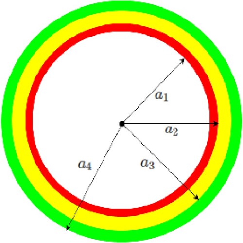
In this section, the bianisotropic susceptibility tensor components of a cylindrical, multilayered, magneto-dielectric shell are extracted. The geometry is shown in Figure 2. Even though a three layered geometry is shown, the method can be used for any number of layers. The medium inside and outside the shell is vacuum. $\mathrm{T}{\mathrm{M}}_{\mathrm{z}}$ polarization is assumed. Following Equation (4) in [10], the differential field components across the cylindrical metasurface $\mathrm{\Delta }{E}_z,\mathrm{\Delta }{H}_{\varphi },\mathrm{\Delta }{H}_z,\mathrm{\Delta }{E}_{\varphi }$ are related to the average of fields across the metasurface $E_{z,\mathrm{av}},H_{\varphi ,\mathrm{av}},E_{\varphi ,\mathrm{av}},H_{z,\mathrm{av}},$ through the following metasurface synthesis expressions: (16a) $\begin{array}{rl}& \begin{array}{rl}& \left[\begin{array}{c}-\mathrm{\Delta }{H}_z\\ \mathrm{\Delta }{H}_{\varphi }\end{array}\right]=j\omega {ϵ}_0\left[\begin{array}{cc}{\chi }_{\mathrm{ee}}^{\varphi \varphi }& {\chi }_{\mathrm{ee}}^{\varphi z}\\ {\chi }_{\mathrm{ee}}^{z\varphi }& {\chi }_{\mathrm{ee}}^{zz}\end{array}\right]\left[\begin{array}{c}{E}_{\varphi ,\mathrm{av}}\\ E_{z,\mathrm{av}}\end{array}\right]+j\omega \sqrt{{\mu }_0{ϵ}_0}\end{array}\end{array}$(16a) (16b) $\begin{array}{rl}& \begin{array}{rl}& \left[\begin{array}{cc}{\chi }_{\mathrm{em}}^{\varphi \varphi }& {\chi }_{\mathrm{em}}^{\varphi z}\\ {\chi }_{\mathrm{em}}^{z\varphi }& {\chi }_{\mathrm{em}}^{zz}\end{array}\right]\left[\begin{array}{c}{H}_{\varphi ,\mathrm{av}}\\ H_{z,\mathrm{av}}\end{array}\right]\end{array}\end{array}$(16b) (16c) $\begin{array}{rl}& \begin{array}{rl}& \left[\begin{array}{c}\mathrm{\Delta }{E}_z\\ -\mathrm{\Delta }{E}_{\varphi }\end{array}\right]=j\omega \sqrt{{\mu }_0{ϵ}_0}\left[\begin{array}{cc}{\chi }_{\mathrm{me}}^{\varphi \varphi }& {\chi }_{\mathrm{me}}^{\varphi z}\\ {\chi }_{\mathrm{me}}^{z\varphi }& {\chi }_{\mathrm{me}}^{zz}\end{array}\right]\left[\begin{array}{c}{E}_{\varphi ,\mathrm{av}}\\ E_{z,\mathrm{av}}\end{array}\right]+j\omega {\mu }_0\end{array}\end{array}$(16c) (16d) $\begin{array}{r}\begin{array}{rl}& \left[\begin{array}{cc}{\chi }_{\mathrm{mm}}^{\varphi \varphi }& {\chi }_{\mathrm{mm}}^{\varphi z}\\ {\chi }_{\mathrm{mm}}^{z\varphi }& {\chi }_{\mathrm{mm}}^{zz}\end{array}\right]\left[\begin{array}{c}{H}_{\varphi ,\mathrm{av}}\\ H_{z,\mathrm{av}}\end{array}\right]\end{array}\end{array}$(16d) For the case of $\mathrm{T}{\mathrm{M}}_{\mathrm{z}}$ polarization, they reduce to (17a) $\begin{array}{rl}\mathrm{\Delta }{E}_z& =j\omega \sqrt{{\mu }_0{ϵ}_0}{\chi }_{\mathrm{me}}^{\varphi z}{E}_{z,\mathrm{av}}+j\omega {\mu }_0{\chi }_{\mathrm{mm}}^{\varphi \varphi }{H}_{\varphi ,\mathrm{av}}\end{array}$(17a) (17b) $\begin{array}{rl}\mathrm{\Delta }{H}_{\varphi }& =j\omega {ϵ}_0{\chi }_{\mathrm{ee}}^{zz}{E}_{z,\mathrm{av}}+j\omega \sqrt{{\mu }_0{ϵ}_0}{\chi }_{\mathrm{em}}^{z\varphi }{H}_{\varphi ,\mathrm{av}}\end{array}$(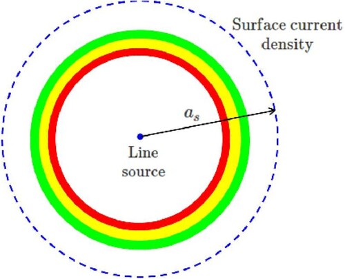17b) Since there are four unknown susceptibility components in the above equation, two different excitation problems are solved to obtain the four susceptibility components. The two excitations used are shown in Figure 3. The first excitation is that of an infinite, electric line source at the origin and the second excitation problem is that of a cylindrical surface electric current density of radius $a_s$, where $a_s>a_4$. The two scattering problems are simple boundary value problems, which can be either solved analytically [26] or simulated using COMSOL. In the case of analytical solution, the vector magnetic potential, electric field and magnetic field in each region can be expressed in terms of Bessel functions: (18a) $\begin{array}{rl}{A}_{z,i}\left(\rho \right)& =C_i{J}_0(k_i\rho )+D_i{Y}_0(k_i\rho )\end{array}$(18a) (18b) $\begin{array}{rl}{E}_{z,i}\left(\rho \right)& =-j\omega [C_i{J}_0(k_i\rho )+D_i{Y}_0(k_i\rho )]\end{array}$(18b) (18c) $\begin{array}{rl}{H}_{\varphi ,i}\left(\rho \right)& =\frac{k_i}{{\mu }_i}[C_i{J}_1(k_i\rho )+D_i{Y}_1(k_i\rho )]\end{array}$(18c) where $J_0(\cdot ),Y_0(\cdot )$ are Bessel functions of the first and second kind, respectively. $k_i,{\mu }_i$ are the wavenumber and permeability of region i. For the case of a cylindrical surface current density excitation of the three layered, magneto-dielectric cylinder, the total number of regions is 6 (the surface current density discontinuity splits the external medium into two separate regions). Applying the continuity of electric and magnetic fields across the region boundaries and the magnetic field discontinuity caused by surface current density, the unknowns $C_i,D_i$ can be obtained. Details of this problem can be found in Appendix.

Figure 2. Three layered cylindrical, magneto-dielectric shell.

This figure shows a concentric, 3 layered, circular shell. There are three rings each denoting different materials. The innermost region (inside the three layered shell) is vacuum and the region outside the 3 layers is also vacuum.

Once the two excitation problems are solved, the susceptibility tensor components are obtained as follows (19) $$\begin{gathered} j\frac{\omega }{c_0}\left[\begin{array}{cccc}{E}_{z,\mathrm{av}}^{(1)}& {\eta }_0{H}_{\varphi ,\mathrm{av}}^{(1)}& 0& 0\\ 0& 0& {\displaystyle \frac{E_{z,\mathrm{av}}^{(1)}}{{\eta }_0}}& H_{\varphi ,\mathrm{av}}^{(1)}\\ E_{z,\mathrm{av}}^{(2)}& {\eta }_0{H}_{\varphi ,\mathrm{av}}^{(2)}& 0& 0\\ 0& 0& {\displaystyle \frac{E_{z,\mathrm{av}}^{(2)}}{{\eta }_0}}& H_{\varphi ,\mathrm{av}}^{(2)}\end{array}\right]\left[\begin{array}{c}{\chi }_{\mathrm{me}}^{\varphi z}\\ {\chi }_{\mathrm{mm}}^{\varphi \varphi }\\ {\chi }_{\mathrm{ee}}^{zz}\\ {\chi }_{\mathrm{em}}^{z\varphi }\end{array}\right]= \\ \left[\begin{array}{c}\mathrm{\Delta }{E}_z^{(1)}\\ \mathrm{\Delta }{H}_{\varphi }^{(1)}\\ \mathrm{\Delta }{E}_z^{(2)}\\ \mathrm{\Delta }{H}_{\varphi }^{(2)}\end{array}\right] \end{gathered}$$(19) where the superscript (1) denotes line source excitation fields and (2) denotes the cylindrical surface current density excitation. It should be noted that the magneto-dielectric shells and excitations considered are azimuthally invariant, hence the resultant tangential fields and the extracted susceptibilities have no dependance along the ϕ direction.

Figure 3. Bianisotropic susceptibility tensor extraction using two sources: (1) Infinite electric line source at origin, $\overline{J}=\delta (x)\delta (y)\hat{z}\mathrm{A}{\mathrm{m}}^{-2}$ shown as a blue dot (2) Cylindrical electric surface current density of radius $a_s$, ${\overline{J}}_s=\delta (\rho -a_s)\hat{z}\mathrm{A}{\mathrm{m}}^{-1}$ shown as a dashed, blue circle.

This figure is similar to Figure 2. It shows two excitations for extracting susceptibility tensor. There is a dashed circle outside the 3 layers. This dashed circle represents a surface electric current density distribution. Its radius is a subscript s. At the center of the inner most region, there is a dot which represents a line source.

4. Numerical validation

This section contain examples of cylindrical metasurface scattering problems. Simulation results obtained from IE-GSTC and susceptibility extraction method described in the previous sections are compared with full wave simulation results obtained using FEM based COMSOL software.

4.1. Four segment cylindrical metasurface excited by plane wave

The cylindrical metasurface shown in Figure 4 consists of four segments (quadrants). Each segment is a multilayered, concentric, magneto-dielectric shell. The susceptibility tensor components of each segment can be extracted using the method in the previous section. Referring to Figure 4, different annular regions are identified as follows: region 1: $0\le \rho <a_1$, region 2: $a_1\le \rho <a_2$, region 3: $a_2\le \rho <a_3$, region 4: $a_3\le \rho <a_4$ and region 5: $a_4\le \rho <\mathrm{\infty }$. The metasurface is surrounded by vacuum, i.e. region 1 and region 5 are vacuum. The material properties of each region (represented by subscript number) in the four quadrants are given in Table 1. The susceptibility tensors of the quadrants are also given. The dimensions are: $a_1=5\lambda$, $a_2=5\lambda +\frac{\lambda }{24}$, $a_3=a_2+\frac{\lambda }{24}$, $a_4=a_3+\frac{\lambda }{20}$. The susceptibility component extraction from the last section is performed four times to get the component values of the four metasurface segments. For example, consider the case of obtaining the susceptibility tensor components of the metasurface segment of quadrant 1 of Figure 4. The material properties of the quadrant 1 are listed in Table 1. The process involves excitation using line source and circular source of an azimuthally invariant shell structure in Figure 3. The material properties of each layer in Figure 3 corresponds to those given in Table 1 for quadrant 1. The same procedure is repeated for other metasurface segments. In the IE-GSTC code, the matrix A of (4a(4a) $\begin{array}{rl}{\mathbf{F}}_{\mathbf{2}}({\overline{\rho }}_{\mathbf{2}}^{\mathrm{\prime }})& =\mathbf{A}({\overline{\rho }}_{\mathbf{c}}^{\mathrm{\prime }}){\mathbf{F}}_{\mathbf{1}}({\overline{\rho }}_{\mathbf{1}}^{\mathrm{\prime }})\end{array}$(4a) ) is varied depending on the position. For instance, for the first quadrant, A is calculated using tensor components in the first row of Table 1.

Figure 4. Four segment cylindrical metasurface.

This figure shows the cylindrical metasurface used in example 4.1. Example 4.1 is titled: four segment cylindrical metasurface excited by plane wave. This figure consists of four quadrants of concentric, 3 layered shells. The radius of shells in increasing values are a1, a2, a3 and a4.

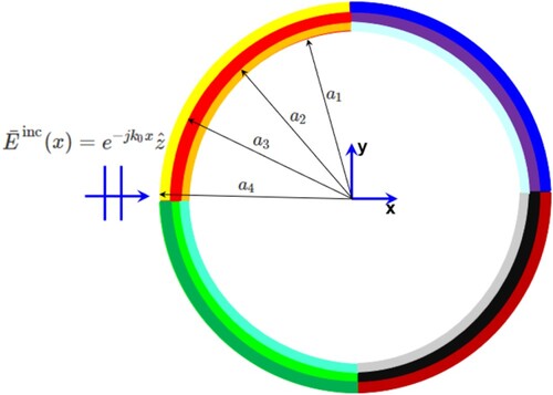
Table 1. Material properties and susceptibility tensor of metasurface segments in Figure 4. Permittivity and permeability have subscripts which represent corresponding regions.

Quadrant	Material properties	Susceptibility tensor
Quadrant 1	${ϵ}_{r1}=1,{\mu }_{r1}=1$	${\chi }_{\mathrm{me}}^{\varphi z}=j2.55236\times {10}^{-3}$
	${ϵ}_{r2}=9,{\mu }_{r2}=2$	${\chi }_{\mathrm{mm}}^{\varphi \varphi }=6.08697\times {10}^{-2}$
	${ϵ}_{r3}=4,{\mu }_{r3}=1$	${\chi }_{\mathrm{ee}}^{zz}=1.97682\times {10}^{-1}$
	${ϵ}_{r4}=9,{\mu }_{r4}=2$	${\chi }_{\mathrm{em}}^{z\varphi }=j1.42107\times {10}^{-2}$
	${ϵ}_{r5}=1,{\mu }_{r5}=1$
Quadrant 2	${ϵ}_{r1}=1,{\mu }_{r1}=1$	${\chi }_{\mathrm{me}}^{\varphi z}=-j1.79047\times {10}^{-5}$
	${ϵ}_{r2}=4,{\mu }_{r2}=1$	${\chi }_{\mathrm{mm}}^{\varphi \varphi }=5.27727\times {10}^{-3}$
	${ϵ}_{r3}=3,{\mu }_{r3}=1$	${\chi }_{\mathrm{ee}}^{zz}=1.86202\times {10}^{-2}$
	${ϵ}_{r4}=4,{\mu }_{r4}=1$	${\chi }_{\mathrm{em}}^{z\varphi }=j2.78948\times {10}^{-4}$
	${ϵ}_{r5}=1,{\mu }_{r5}=1$
Quadrant 3	${ϵ}_{r1}=1,{\mu }_{r1}=1$	${\chi }_{\mathrm{me}}^{\varphi z}=j1.45598\times {10}^{-3}$
	${ϵ}_{r2}=4,{\mu }_{r2}=1$	${\chi }_{\mathrm{mm}}^{\varphi \varphi }=9.25367\times {10}^{-3}$
	${ϵ}_{r3}=3,{\mu }_{r3}=1$	${\chi }_{\mathrm{ee}}^{zz}=2.80732\times {10}^{-2}$
	${ϵ}_{r4}=6,{\mu }_{r4}=2$	${\chi }_{\mathrm{em}}^{z\varphi }=-j9.74236\times {10}^{-4}$
	${ϵ}_{r5}=1,{\mu }_{r5}=1$
Quadrant 4	${ϵ}_{r1}=1,{\mu }_{r1}=1$	${\chi }_{\mathrm{me}}^{\varphi z}=j2.83566\times {10}^{-4}$
	${ϵ}_{r2}=1,{\mu }_{r2}=1$	${\chi }_{\mathrm{mm}}^{\varphi \varphi }=6.01626\times {10}^{-3}$
	${ϵ}_{r3}=6,{\mu }_{r3}=2$	${\chi }_{\mathrm{ee}}^{zz}=1.44824\times {10}^{-2}$
	${ϵ}_{r4}=1,{\mu }_{r4}=1$	${\chi }_{\mathrm{em}}^{z\varphi }=-j3.78786\times {10}^{-5}$
	${ϵ}_{r5}=1,{\mu }_{r5}=1$

Alt text: This table provides the material properties (i.e. permittivity and permeability) of the materials used in the 4 quadrant, 3 layered cylindrical metasurface of example 4.1. The table has three columns. The first column shows the quadrant number (i.e quandrant 1, 2, 3 and 4). The second column gives the permittivity and permeability of each layer. The layers are denoted by subscripts 1, 2, 3, 4 and 5. Subscripts 1 and 5 denote the innermost and outermost region, respectively. The third column shows the susceptibility tensor component of each segment.

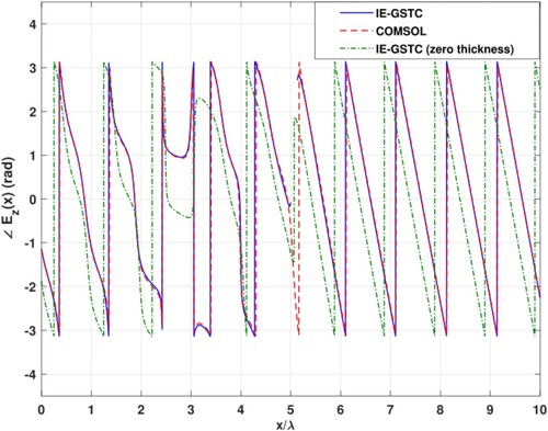
The structure is excited by a plane wave, ${\overline{E}}^{\mathrm{inc}}(x)=e^{-j{k}_{0}x}\hat{z}$. The total field along a line from $(0,0)$ to $(10\lambda ,0)$ is plotted in Figures 5 and 6. There is good agreement between IE-GSTC and full wave results obtained using COMSOL software. For the IE-GSTC result a small gap can be observed around the metasurface radius of $x=5\lambda$. This is because IE results is valid only for regions interior and exterior to the metasurface. Minor discrepancies between the two results can be seen around the metasurface. This is probably due to MoM being inefficient in the near field of the scatterer as well as GSTC being an approximate interface condition. In Figures 5 and 6, the results from the zero-thickness IE-GSTC [10] are plotted for the same problem to show that the formulation in this paper is required to get more accurate results. COMSOL discretizes and solves the fields inside the thin dielectric layers, while IE-GSTC abstracts it. This is the advantage of using IE-GSTC.

Figure 5. IE-GSTC vs. full wave simulation for example Section 4.1. $|E_z(x)|$ vs. x from $(0,0)$ to $(10\lambda ,0)$.

This figure compares result of IE-GSTC applied to example 4.1 with commercially available CAD software COMSOL. The y-axis is the magnitude of z-component of electric field along a horizontal line from center of the structure to a point outside the metasurface. The length of the line is about 10 wavelengths. Good agreement between the two plots can be seen.

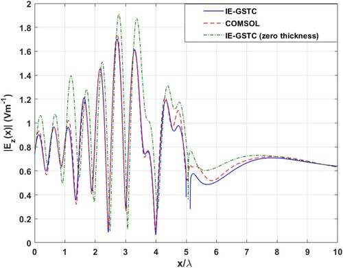
Figure 6. IE-GSTC vs. full wave simulation for example Section 4.1. $\mathrm{\angle }{E}_z(x)$ vs. x from $(0,0)$ to $(10\lambda ,0)$.

This figure compares result of IE-GSTC applied to example 4.1 with commercially available CAD software COMSOL. The y-axis is the phase of z-component of electric field along a horizontal line from center of the structure to a point outside the metasurface. The length of the line is about 10 wavelengths. Good agreement between the two plots can be seen.

In Table 1, it can be seen that even though the metasurface elements are passive, lossless and reciprocal the condition ${\chi }_{\mathrm{me}}^{\varphi z}=-{\chi }_{\mathrm{em}}^{z\varphi }$ as stated in [14] is not satisfied. In [14], Figure 4 shows a unit cell characterization system in which a curved, spherical metasurface particle is illuminated by both inward propagating and outward propagating spherical waves. The susceptibility extraction technique in this paper is essentially an analytical, cylindrical version of the numerical, spherical system shown in Figure 4 in [14]. As stated in [14], the condition ${\chi }_{\mathrm{me}}^{\varphi z}=-{\chi }_{\mathrm{em}}^{z\varphi }$ is not satisfied because of the curvature, that is, the inner contour of the scattering particle is not of the same length as its outer contour. The inner contour length becomes approximately equal to the outer contour length only when the radius of curvature is very large. This can be proved numerically with the susceptibility extraction method described in the last section. In Table 2, the susceptibility tensor components of the metasurface element in quadrant I are shown as the inner radius $a_1$ is varied. It can be seen that for large radius of curvature, the condition is approximately satisfied. The results of the susceptibility extraction are robust with respect to different illuminations. For instance, changing the value of outer surface current excitation i.e. $a_s$ in Figure 3 gives the same results. Furthermore, a one dimensional cylindrical FDTD code [27] was developed to independently obtain the results. A one dimensional cylindrical FDTD with variation along the ρ direction and no variation along ϕ, z directions will automatically take the curvature into account.The condition that the metasurface particle should have an electrically large curvature to satisfy the reciprocity condition is stated in a footnote in [14].

Table 2. Susceptibility tensor components of quadrant 1 in Figure 4. as a function of radius.

Metasurface radius	Susceptibility tensor
$a_1=5\lambda$	${\chi }_{\mathrm{me}}^{\varphi z}=j2.55236\times {10}^{-3}$
	${\chi }_{\mathrm{em}}^{z\varphi }=j1.4211\times {10}^{-2}$
$a_1=20\lambda$	${\chi }_{\mathrm{me}}^{\varphi z}=-j2.4572\times {10}^{-3}$
	${\chi }_{\mathrm{em}}^{z\varphi }=j6.7137\times {10}^{-3}$
$a_1=100\lambda$	${\chi }_{\mathrm{me}}^{\varphi z}=-j3.8152\times {10}^{-3}$
	${\chi }_{\mathrm{em}}^{z\varphi }=j4.6690\times {10}^{-3}$
$a_1=300\lambda$	${\chi }_{\mathrm{me}}^{\varphi z}=-j4.0421\times {10}^{-3}$
	${\chi }_{\mathrm{em}}^{z\varphi }=j4.3268\times {10}^{-3}$

Alt text: In this table, the susceptibility tensor components of metasurface particle in quadrant 1 is listed as a function of the inner radius a1. The radius a1 is varied from 5 wavelengths to 300 wavelengths.

4.2. Cylindrical metasurface with opening excited by a plane wave

This example, as shown in Figure 7, is a four segment metasurface but with an opening. The opening subtends an angle of $\pi /2$ at the center and is equally divided between the first and fourth quadrants. The structure is excited by a plane wave ${\overline{E}}^{\mathrm{inc}}(x)=e^{-j{k}_{0}x}\hat{z}$. The material properties of the quadrants are same as that of the previous example. GSTC cannot handle segments with material properties same as that of the background medium. In the IE-GSTC approach, an opening is handled by setting $\mathbf{A}({\overline{\rho }}_c^{\mathrm{\prime }})$ = $\mathrm{diag}(1,1,1,1)$ [10]. This ensures that tangential fields on either side of the opening are equal. This is only an approximation because the opening has a width of fraction of a wavelength. IE-GSTC results and COMSOL results on a circle of radius $8\lambda$ are plotted in Figures 8 and 9.

Figure 7. Four segment cylindrical metasurface with opening.

This figure shows the metasurface which is used in example 4.2 (i.e. cylindrical metasurface with opening excited by a plane wave). It is a four segment, 3 layered, concentric cylindrical shell. There is an opening that subtends an angle of 90 degrees.

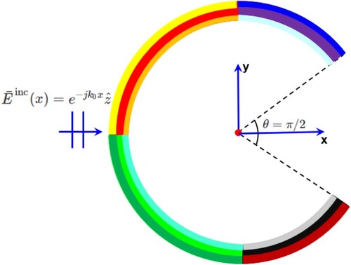
Figure 8. IE-GSTC vs. full wave simulation for example Section 4.2. $|E_z(\varphi )|$ vs. ϕ on a circle of radius $8\lambda$.

This figure compares result of IE-GSTC applied to example 4.2 with commercially available CAD software COMSOL. The y-axis is the phase of z-component of electric field along a circle of radius 8 wavelengths. Good agreement between the two plots can be seen. This figure compares result of IE-GSTC applied to example 4.2 with commercially available CAD software COMSOL. The y-axis is the magnitude of z-component of electric field along a circle of radius 8 wavelengths. Good agreement between the two plots can be seen.

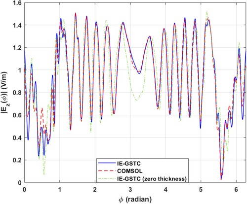
Figure 9. IE-GSTC vs. full wave simulation for example Section 4.2. $\mathrm{\angle }{E}_z(\varphi )$ vs. ϕ on a circle of radius $8\lambda$.

This figure compares result of IE-GSTC applied to example 4.2 with commercially available CAD software COMSOL. The y-axis is the phase of z-component of electric field along a circle of radius 8 wavelengths. Good agreement between the two plots can be seen.

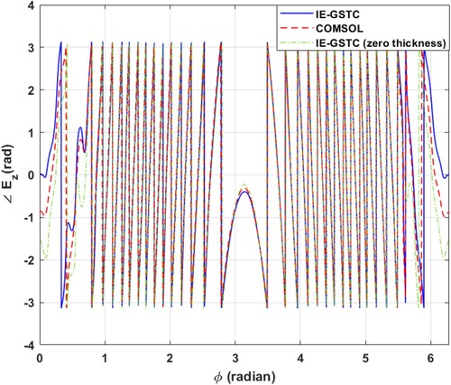
4.3. Eight segment metasurface excited by a line source

In this example, an eight segment cylindrical metasurface with each segment subtending an angle of $\pi /4$ is excited by an infinite electric, line source at origin, i.e. $\overline{J}(\overline{r})=\delta (x)\delta (y)\hat{z}$ $\mathrm{A}{\mathrm{m}}^{-2}$. The dimension of the structure is same as that of the example Section 4.1. The segment angular positions are $[0,\pi /4],[\pi /4,\pi /2]$ and so on. The segments on the top half are exactly the same ones as in Table 1 (Figure 10). The segments on the bottom half is listed in Table 3. The magnitude and phase of the electric field on a circle of radius $8\lambda$ are shown in Figures 8 and  11 respectively. Zero thickness IE-GSTC [10] results are also superimposed. In the COMSOL full wave simulation, the line source is modeled using the external current density option on a circle of radius much smaller than wavelength ($\sim \lambda /100$).

Figure 10. IE-GSTC vs. full wave simulation for example Section 4.3. $|E_z(\varphi )|$ vs. ϕ on a circle of radius $8\lambda$.

This figure compares result of IE-GSTC applied to example 4.3 with results from commercially available CAD software COMSOL. The y-axis is the magnitude of z-component of electric field along a circle of radius 8 wavelengths. Good agreement between the two plots can be seen.

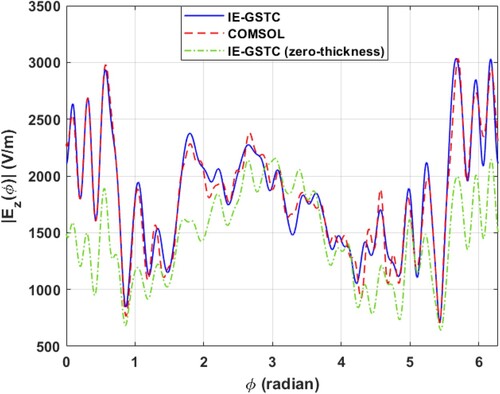
Figure 11. IE-GSTC vs. full wave simulation for example Section 4.3. $\mathrm{\angle }{E}_z(\varphi )$ vs. ϕ on a circle of radius $8\lambda$.

This figure compares result of IE-GSTC applied to example 4.3 with results from commercially available CAD software COMSOL. The y-axis is the phase of z-component of electric field along a circle of radius 8 wavelengths. Good agreement between the two plots can be seen.

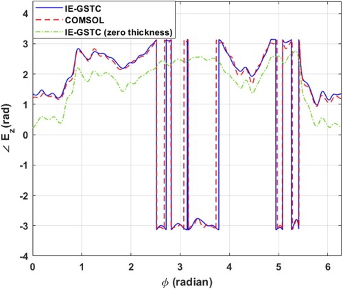
Table 3. Material properties and susceptibility tensor of metasurface segments for lower half of cylindrical metasurface of example Section 4.3. Permittivity and permeability have subscripts which represent corresponding regions.

Quadrant	Material properties	Susceptibility tensor
$\pi \le \varphi <5\pi /4$	${ϵ}_{r1}=1,{\mu }_{r1}=1$	${\chi }_{\mathrm{me}}^{\varphi z}=-j1.50001\times {10}^{-3}$
	${ϵ}_{r2}=1,{\mu }_{r2}=1$	${\chi }_{\mathrm{mm}}^{\varphi \varphi }=4.74909\times {10}^{-3}$
	${ϵ}_{r3}=4,{\mu }_{r3}=1$	${\chi }_{\mathrm{ee}}^{zz}=1.62999\times {10}^{-2}$
	${ϵ}_{r4}=1,{\mu }_{r4}=1$	${\chi }_{\mathrm{em}}^{z\varphi }=j1.72889\times {10}^{-3}$
	${ϵ}_{r5}=1,{\mu }_{r5}=1$
$5\pi /4\le \varphi <3\pi /2$	${ϵ}_{r1}=1,{\mu }_{r1}=1$	${\chi }_{\mathrm{me}}^{\varphi z}=j2.44255\times {10}^{-2}$
	${ϵ}_{r2}=4,{\mu }_{r2}=1$	${\chi }_{\mathrm{mm}}^{\varphi \varphi }=1.31683\times {10}^{-2}$
	${ϵ}_{r3}=10,{\mu }_{r3}=1$	${\chi }_{\mathrm{ee}}^{zz}=1.16977\times {10}^{-1}$
	${ϵ}_{r4}=4,{\mu }_{r4}=2$	${\chi }_{\mathrm{em}}^{z\varphi }=-j2.29491\times {10}^{-2}$
	${ϵ}_{r5}=1,{\mu }_{r5}=1$
$3\pi /2\le \varphi <7\pi /4$	${ϵ}_{r1}=1,{\mu }_{r1}=1$	${\chi }_{\mathrm{me}}^{\varphi z}=j2.19819\times {10}^{-4}$
	${ϵ}_{r2}=1,{\mu }_{r2}=1$	${\chi }_{\mathrm{mm}}^{\varphi \varphi }=4.28646\times {10}^{-3}$
	${ϵ}_{r3}=5,{\mu }_{r3}=1$	${\chi }_{\mathrm{ee}}^{zz}=1.15471\times {10}^{-2}$
	${ϵ}_{r4}=1,{\mu }_{r4}=1$	${\chi }_{\mathrm{em}}^{z\varphi }=-j2.60041\times {10}^{-5}$
	${ϵ}_{r5}=1,{\mu }_{r5}=1$
$7\pi /4\le \varphi <2\pi$	${ϵ}_{r1}=1,{\mu }_{r1}=1$	${\chi }_{\mathrm{me}}^{\varphi z}=j3.14385\times {10}^{-2}$
	${ϵ}_{r2}=10,{\mu }_{r2}=2$	${\chi }_{\mathrm{mm}}^{\varphi \varphi }=-6.54633\times {10}^{-1}$
	${ϵ}_{r3}=4,{\mu }_{r3}=1$	${\chi }_{\mathrm{ee}}^{zz}=4.27841\times {10}^{-1}$
	${ϵ}_{r4}=10,{\mu }_{r4}=2$	${\chi }_{\mathrm{em}}^{z\varphi }=-j4.36316\times {10}^{-1}$
	${ϵ}_{r5}=1,{\mu }_{r5}=1$

Alt text: This table provides the material properties (i.e. permittivity and permeability) of the materials used in the 8 quadrant, 3 layered cylindrical metasurface of example 4.3 (i.e. eight segment metasurface excited by a line source). The table has three columns. The first column shows the segment number. These are segment numbers in the lower half of the metasurface. The second column gives the permittivity and permeability of each layer. The layers are denoted by subscripts 1, 2, 3, 4 and 5. Subscripts 1 and 5 denote the innermost and outermost region, respectively. The third column shows the susceptibility tensor component of each segment.

5. IE-GSTC modeling of cylindrical metasurface -- PEC composite structures

In this section, the IE-GSTC formulation is extended to include PEC segments. GSTC can be used to model dielectric segments, dielectric segments with metallic/non-metallic inclusions, etc. When one of the segments is PEC, the IE-GSTC model needs to be extended. Potential applications include PEC backed metasurface lens antennas, intelligent surface enabled wireless environments [28], and scattering reduction and radiation problems [29].

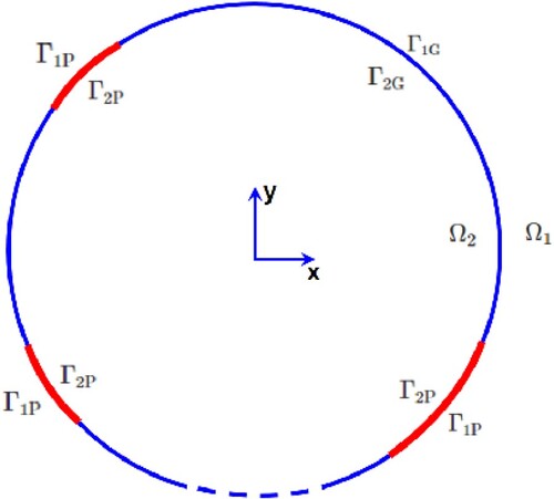
The problem under consideration is shown in Figure 12. Similar to the previous examples, there is no variation of material properties or excitation along the z axis. The inner contour is ${\mathrm{\Gamma }}_2$ and the outer contour is ${\mathrm{\Gamma }}_1$, separated by metasurface thickness δ. The circular boundary which separates the external domain ${\mathrm{\Omega }}_1$ and internal domain ${\mathrm{\Omega }}_2$ is partly GSTC (mathematical abstraction for physical metasurface) and partly PEC. The GSTC part is denoted by $\mathrm{G}$ and the PEC part is denoted by $\mathrm{P}$. Therefore ${\mathrm{\Gamma }}_{1\mathrm{G}}$ and ${\mathrm{\Gamma }}_{1\mathrm{P}}$ represent the outer contour of GSTC and PEC sections. Similarly, ${\mathrm{\Gamma }}_{2\mathrm{G}}$ and ${\mathrm{\Gamma }}_{2\mathrm{P}}$ represent the inner contour of GSTC and PEC sections. The PEC sections do not necessarily need to be contiguous. Considering $\mathrm{T}{\mathrm{M}}_{\mathrm{z}}$ polarization and referring to Figure 12, the governing integral equations read (20a) $\begin{array}{rl}& \frac{E_{z1}({\overline{\rho }}_1)}{2}-{\oint }_{{\mathrm{\Gamma }}_1}[E_{z1}({\overline{\rho }}_1^{\mathrm{\prime }})\frac{\mathrm{\partial }{G}_0({\overline{\rho }}_1;{\overline{\rho }}_1^{\mathrm{\prime }})}{\mathrm{\partial }{n}^{\mathrm{\prime }}}-j\omega {\mu }_0{H}_{\varphi 1}({\overline{\rho }}_1^{\mathrm{\prime }})G_0({\overline{\rho }}_1;{\overline{\rho }}_1^{\mathrm{\prime }})]\mathrm{d}{\mathrm{\Gamma }}_1^{\mathrm{\prime }}\\ & =E_{z1}^{\mathrm{inc}}({\overline{\rho }}_1);{\overline{\rho }}_1\in {\mathrm{\Gamma }}_1\end{array}$(20a) (20b) $\begin{array}{rl}& \frac{E_{z2}({\overline{\rho }}_2)}{2}+{\oint }_{{\mathrm{\Gamma }}_2}[E_{z2}({\overline{\rho }}_2^{\mathrm{\prime }})\frac{\mathrm{\partial }{G}_0({\overline{\rho }}_2;{\overline{\rho }}_2^{\mathrm{\prime }})}{\mathrm{\partial }{n}^{\mathrm{\prime }}}-j\omega {\mu }_0{H}_{\varphi 2}({\overline{\rho }}_2^{\mathrm{\prime }})G_0({\overline{\rho }}_2;{\overline{\rho }}_2^{\mathrm{\prime }})]\mathrm{d}{\mathrm{\Gamma }}_2^{\mathrm{\prime }}\\ & =E_{z2}^{\mathrm{inc}}({\overline{\rho }}_2);{\overline{\rho }}_2\in {\mathrm{\Gamma }}_2\end{array}$(20b) On the GSTC part of the boundary, the external and internal tangential electric and magnetic fields are related through matrix $\mathbf{A}({\overline{\rho }}_c)$ (21) $\left[\begin{array}{c}{E}_{z2}({\overline{\rho }}_2)\\ H_{\varphi 2}({\overline{\rho }}_2)\end{array}\right]=\left[\begin{array}{cc}{A}_{11}({\overline{\rho }}_c)& A_{12}({\overline{\rho }}_c)\\ A_{21}({\overline{\rho }}_c)& A_{22}({\overline{\rho }}_c)\end{array}\right]\left[\begin{array}{c}{E}_{z1}({\overline{\rho }}_1)\\ H_{\varphi 1}({\overline{\rho }}_1)\end{array}\right]$(21) where ${\overline{\rho }}_c$ denotes the center of the metasurface, i.e. ${\overline{\rho }}_c={\overline{\rho }}_1-0.5\delta \hat{\rho }$. For PEC segments, there is no relation between the tangential components on the inner and outer domains. By using the fact that the total tangential electric field on the PEC surface is zero, the integral Equation (20a(20a) $\begin{array}{rl}& \frac{E_{z1}({\overline{\rho }}_1)}{2}-{\oint }_{{\mathrm{\Gamma }}_1}[E_{z1}({\overline{\rho }}_1^{\mathrm{\prime }})\frac{\mathrm{\partial }{G}_0({\overline{\rho }}_1;{\overline{\rho }}_1^{\mathrm{\prime }})}{\mathrm{\partial }{n}^{\mathrm{\prime }}}-j\omega {\mu }_0{H}_{\varphi 1}({\overline{\rho }}_1^{\mathrm{\prime }})G_0({\overline{\rho }}_1;{\overline{\rho }}_1^{\mathrm{\prime }})]\mathrm{d}{\mathrm{\Gamma }}_1^{\mathrm{\prime }}\\ & =E_{z1}^{\mathrm{inc}}({\overline{\rho }}_1);{\overline{\rho }}_1\in {\mathrm{\Gamma }}_1\end{array}$(20a) ) is converted to two IEs, one for ${\overline{\rho }}_1\in {\mathrm{\Gamma }}_{1\mathrm{G}}$ and another for ${\overline{\rho }}_1\in {\mathrm{\Gamma }}_{1\mathrm{P}}$: (22a) $\begin{array}{rl}& \frac{E_{z1}({\overline{\rho }}_1)}{2}-{\int }_{{\mathrm{\Gamma }}_{1\mathrm{G}}}[E_{z1}({\overline{\rho }}_1^{\mathrm{\prime }})\frac{\mathrm{\partial }{G}_0({\overline{\rho }}_1;{\overline{\rho }}_1^{\mathrm{\prime }})}{\mathrm{\partial }{n}^{\mathrm{\prime }}}-j\omega {\mu }_0{H}_{\varphi 1}({\overline{\rho }}_1^{\mathrm{\prime }})G_0({\overline{\rho }}_1;{\overline{\rho }}_1^{\mathrm{\prime }})]\mathrm{d}{\mathrm{\Gamma }}_1^{\mathrm{\prime }}\\ & -{\int }_{{\mathrm{\Gamma }}_{1\mathrm{P}}}[-j\omega {\mu }_0{H}_{\varphi 1}({\overline{\rho }}_1^{\mathrm{\prime }})G_0({\overline{\rho }}_1;{\overline{\rho }}_1^{\mathrm{\prime }})]\mathrm{d}{\mathrm{\Gamma }}_1^{\mathrm{\prime }}=E_{z1}^{\mathrm{inc}}({\overline{\rho }}_1);{\overline{\rho }}_1\in {\mathrm{\Gamma }}_{1\mathrm{G}}\end{array}$(22a) (22b) $\begin{array}{rl}& -{\int }_{{\mathrm{\Gamma }}_{1\mathrm{G}}}[E_{z1}({\overline{\rho }}_1^{\mathrm{\prime }})\frac{\mathrm{\partial }{G}_0({\overline{\rho }}_1;{\overline{\rho }}_1^{\mathrm{\prime }})}{\mathrm{\partial }{n}^{\mathrm{\prime }}}-j\omega {\mu }_0{H}_{\varphi 1}({\overline{\rho }}_1^{\mathrm{\prime }})G_0({\overline{\rho }}_1;{\overline{\rho }}_1^{\mathrm{\prime }})]\mathrm{d}{\mathrm{\Gamma }}_1^{\mathrm{\prime }}\\ & -{\int }_{{\mathrm{\Gamma }}_{1\mathrm{P}}}[-j\omega {\mu }_0{H}_{\varphi 1}({\overline{\rho }}_1^{\mathrm{\prime }})G_0({\overline{\rho }}_1;{\overline{\rho }}_1^{\mathrm{\prime }})]\mathrm{d}{\mathrm{\Gamma }}_1^{\mathrm{\prime }}=E_{z1}^{\mathrm{inc}}({\overline{\rho }}_1);{\overline{\rho }}_1\in {\mathrm{\Gamma }}_{1\mathrm{P}}\end{array}$(22b) By using Equation (21(21) $\left[\begin{array}{c}{E}_{z2}({\overline{\rho }}_2)\\ H_{\varphi 2}({\overline{\rho }}_2)\end{array}\right]=\left[\begin{array}{cc}{A}_{11}({\overline{\rho }}_c)& A_{12}({\overline{\rho }}_c)\\ A_{21}({\overline{\rho }}_c)& A_{22}({\overline{\rho }}_c)\end{array}\right]\left[\begin{array}{c}{E}_{z1}({\overline{\rho }}_1)\\ H_{\varphi 1}({\overline{\rho }}_1)\end{array}\right]$(21) ) and the condition that the total tangential electric field on the PEC surface is zero, (20b(20b) $\begin{array}{rl}& \frac{E_{z2}({\overline{\rho }}_2)}{2}+{\oint }_{{\mathrm{\Gamma }}_2}[E_{z2}({\overline{\rho }}_2^{\mathrm{\prime }})\frac{\mathrm{\partial }{G}_0({\overline{\rho }}_2;{\overline{\rho }}_2^{\mathrm{\prime }})}{\mathrm{\partial }{n}^{\mathrm{\prime }}}-j\omega {\mu }_0{H}_{\varphi 2}({\overline{\rho }}_2^{\mathrm{\prime }})G_0({\overline{\rho }}_2;{\overline{\rho }}_2^{\mathrm{\prime }})]\mathrm{d}{\mathrm{\Gamma }}_2^{\mathrm{\prime }}\\ & =E_{z2}^{\mathrm{inc}}({\overline{\rho }}_2);{\overline{\rho }}_2\in {\mathrm{\Gamma }}_2\end{array}$(20b) ) is transformed to two equations, one for ${\overline{\rho }}_2\in {\mathrm{\Gamma }}_{2\mathrm{G}}$ and another for ${\overline{\rho }}_2\in {\mathrm{\Gamma }}_{2\mathrm{P}}$: (23a) $\begin{array}{rl}& \frac{1}{2}[A_{11}({\overline{\rho }}_c)E_{z1}({\overline{\rho }}_1)+A_{12}({\overline{\rho }}_c)H_{\varphi 1}({\overline{\rho }}_1)]+{\int }_{{\mathrm{\Gamma }}_{2\mathrm{G}}}[A_{11}({\overline{\rho }}_c^{\mathrm{\prime }})E_{z1}({\overline{\rho }}_1^{\mathrm{\prime }})+A_{12}({\overline{\rho }}_c^{\mathrm{\prime }})H_{\varphi 1}({\overline{\rho }}_1^{\mathrm{\prime }})]\\ & \times \frac{\mathrm{\partial }{G}_0({\overline{\rho }}_2;{\overline{\rho }}_2^{\mathrm{\prime }})}{\mathrm{\partial }{n}^{\mathrm{\prime }}}\mathrm{d}{\mathrm{\Gamma }}_2^{\mathrm{\prime }}+{\int }_{{\mathrm{\Gamma }}_{2\mathrm{G}}}-j\omega {\mu }_0[A_{21}({\overline{\rho }}_c^{\mathrm{\prime }})E_{z1}({\overline{\rho }}_1^{\mathrm{\prime }})+A_{22}({\overline{\rho }}_c^{\mathrm{\prime }})H_{\varphi 1}({\overline{\rho }}_1^{\mathrm{\prime }})]G_0({\overline{\rho }}_2;{\overline{\rho }}_2^{\mathrm{\prime }})\mathrm{d}{\mathrm{\Gamma }}_2^{\mathrm{\prime }}\\ & +{\int }_{{\mathrm{\Gamma }}_{2\mathrm{P}}}-j\omega {\mu }_0{H}_{\varphi 2}({\overline{\rho }}_2^{\mathrm{\prime }})G_0({\overline{\rho }}_2;{\overline{\rho }}_2^{\mathrm{\prime }})\mathrm{d}{\mathrm{\Gamma }}_2^{\mathrm{\prime }}=E_{z2}^{\mathrm{inc}}({\overline{\rho }}_2);{\overline{\rho }}_2\in {\mathrm{\Gamma }}_{2\mathrm{G}}\end{array}$(23a) (23b) $\begin{array}{rl}& {\int }_{{\mathrm{\Gamma }}_{2\mathrm{G}}}[A_{11}({\overline{\rho }}_c^{\mathrm{\prime }})E_{z1}({\overline{\rho }}_1^{\mathrm{\prime }})+A_{12}({\overline{\rho }}_c^{\mathrm{\prime }})H_{\varphi 1}({\overline{\rho }}_1^{\mathrm{\prime }})]\frac{\mathrm{\partial }{G}_0({\overline{\rho }}_2;{\overline{\rho }}_2^{\mathrm{\prime }})}{\mathrm{\partial }{n}^{\mathrm{\prime }}}\mathrm{d}{\mathrm{\Gamma }}_2^{\mathrm{\prime }}-{\int }_{{\mathrm{\Gamma }}_{2\mathrm{G}}}j\omega {\mu }_0[A_{21}({\overline{\rho }}_c^{\mathrm{\prime }})E_{z1}({\overline{\rho }}_1^{\mathrm{\prime }})\\ & +A_{22}({\overline{\rho }}_c^{\mathrm{\prime }})H_{\varphi 1}({\overline{\rho }}_1^{\mathrm{\prime }})]G_0({\overline{\rho }}_2;{\overline{\rho }}_2^{\mathrm{\prime }})\mathrm{d}{\mathrm{\Gamma }}_2^{\mathrm{\prime }}+{\int }_{{\mathrm{\Gamma }}_{2\mathrm{P}}}-j\omega {\mu }_0{H}_{\varphi 2}({\overline{\rho }}_2^{\mathrm{\prime }})G_0({\overline{\rho }}_2;{\overline{\rho }}_2^{\mathrm{\prime }})\mathrm{d}{\mathrm{\Gamma }}_2^{\mathrm{\prime }}\\ & =E_{z2}^{\mathrm{inc}}({\overline{\rho }}_2);{\overline{\rho }}_2\in {\mathrm{\Gamma }}_{2\mathrm{P}}\end{array}$(23b) The four Equations (22a(22a) $\begin{array}{rl}& \frac{E_{z1}({\overline{\rho }}_1)}{2}-{\int }_{{\mathrm{\Gamma }}_{1\mathrm{G}}}[E_{z1}({\overline{\rho }}_1^{\mathrm{\prime }})\frac{\mathrm{\partial }{G}_0({\overline{\rho }}_1;{\overline{\rho }}_1^{\mathrm{\prime }})}{\mathrm{\partial }{n}^{\mathrm{\prime }}}-j\omega {\mu }_0{H}_{\varphi 1}({\overline{\rho }}_1^{\mathrm{\prime }})G_0({\overline{\rho }}_1;{\overline{\rho }}_1^{\mathrm{\prime }})]\mathrm{d}{\mathrm{\Gamma }}_1^{\mathrm{\prime }}\\ & -{\int }_{{\mathrm{\Gamma }}_{1\mathrm{P}}}[-j\omega {\mu }_0{H}_{\varphi 1}({\overline{\rho }}_1^{\mathrm{\prime }})G_0({\overline{\rho }}_1;{\overline{\rho }}_1^{\mathrm{\prime }})]\mathrm{d}{\mathrm{\Gamma }}_1^{\mathrm{\prime }}=E_{z1}^{\mathrm{inc}}({\overline{\rho }}_1);{\overline{\rho }}_1\in {\mathrm{\Gamma }}_{1\mathrm{G}}\end{array}$(22a) ), (22b(22b) $\begin{array}{rl}& -{\int }_{{\mathrm{\Gamma }}_{1\mathrm{G}}}[E_{z1}({\overline{\rho }}_1^{\mathrm{\prime }})\frac{\mathrm{\partial }{G}_0({\overline{\rho }}_1;{\overline{\rho }}_1^{\mathrm{\prime }})}{\mathrm{\partial }{n}^{\mathrm{\prime }}}-j\omega {\mu }_0{H}_{\varphi 1}({\overline{\rho }}_1^{\mathrm{\prime }})G_0({\overline{\rho }}_1;{\overline{\rho }}_1^{\mathrm{\prime }})]\mathrm{d}{\mathrm{\Gamma }}_1^{\mathrm{\prime }}\\ & -{\int }_{{\mathrm{\Gamma }}_{1\mathrm{P}}}[-j\omega {\mu }_0{H}_{\varphi 1}({\overline{\rho }}_1^{\mathrm{\prime }})G_0({\overline{\rho }}_1;{\overline{\rho }}_1^{\mathrm{\prime }})]\mathrm{d}{\mathrm{\Gamma }}_1^{\mathrm{\prime }}=E_{z1}^{\mathrm{inc}}({\overline{\rho }}_1);{\overline{\rho }}_1\in {\mathrm{\Gamma }}_{1\mathrm{P}}\end{array}$(22b) ), (23a(23a) $\begin{array}{rl}& \frac{1}{2}[A_{11}({\overline{\rho }}_c)E_{z1}({\overline{\rho }}_1)+A_{12}({\overline{\rho }}_c)H_{\varphi 1}({\overline{\rho }}_1)]+{\int }_{{\mathrm{\Gamma }}_{2\mathrm{G}}}[A_{11}({\overline{\rho }}_c^{\mathrm{\prime }})E_{z1}({\overline{\rho }}_1^{\mathrm{\prime }})+A_{12}({\overline{\rho }}_c^{\mathrm{\prime }})H_{\varphi 1}({\overline{\rho }}_1^{\mathrm{\prime }})]\\ & \times \frac{\mathrm{\partial }{G}_0({\overline{\rho }}_2;{\overline{\rho }}_2^{\mathrm{\prime }})}{\mathrm{\partial }{n}^{\mathrm{\prime }}}\mathrm{d}{\mathrm{\Gamma }}_2^{\mathrm{\prime }}+{\int }_{{\mathrm{\Gamma }}_{2\mathrm{G}}}-j\omega {\mu }_0[A_{21}({\overline{\rho }}_c^{\mathrm{\prime }})E_{z1}({\overline{\rho }}_1^{\mathrm{\prime }})+A_{22}({\overline{\rho }}_c^{\mathrm{\prime }})H_{\varphi 1}({\overline{\rho }}_1^{\mathrm{\prime }})]G_0({\overline{\rho }}_2;{\overline{\rho }}_2^{\mathrm{\prime }})\mathrm{d}{\mathrm{\Gamma }}_2^{\mathrm{\prime }}\\ & +{\int }_{{\mathrm{\Gamma }}_{2\mathrm{P}}}-j\omega {\mu }_0{H}_{\varphi 2}({\overline{\rho }}_2^{\mathrm{\prime }})G_0({\overline{\rho }}_2;{\overline{\rho }}_2^{\mathrm{\prime }})\mathrm{d}{\mathrm{\Gamma }}_2^{\mathrm{\prime }}=E_{z2}^{\mathrm{inc}}({\overline{\rho }}_2);{\overline{\rho }}_2\in {\mathrm{\Gamma }}_{2\mathrm{G}}\end{array}$(23a) ) and (23b(23b) $\begin{array}{rl}& {\int }_{{\mathrm{\Gamma }}_{2\mathrm{G}}}[A_{11}({\overline{\rho }}_c^{\mathrm{\prime }})E_{z1}({\overline{\rho }}_1^{\mathrm{\prime }})+A_{12}({\overline{\rho }}_c^{\mathrm{\prime }})H_{\varphi 1}({\overline{\rho }}_1^{\mathrm{\prime }})]\frac{\mathrm{\partial }{G}_0({\overline{\rho }}_2;{\overline{\rho }}_2^{\mathrm{\prime }})}{\mathrm{\partial }{n}^{\mathrm{\prime }}}\mathrm{d}{\mathrm{\Gamma }}_2^{\mathrm{\prime }}-{\int }_{{\mathrm{\Gamma }}_{2\mathrm{G}}}j\omega {\mu }_0[A_{21}({\overline{\rho }}_c^{\mathrm{\prime }})E_{z1}({\overline{\rho }}_1^{\mathrm{\prime }})\\ & +A_{22}({\overline{\rho }}_c^{\mathrm{\prime }})H_{\varphi 1}({\overline{\rho }}_1^{\mathrm{\prime }})]G_0({\overline{\rho }}_2;{\overline{\rho }}_2^{\mathrm{\prime }})\mathrm{d}{\mathrm{\Gamma }}_2^{\mathrm{\prime }}+{\int }_{{\mathrm{\Gamma }}_{2\mathrm{P}}}-j\omega {\mu }_0{H}_{\varphi 2}({\overline{\rho }}_2^{\mathrm{\prime }})G_0({\overline{\rho }}_2;{\overline{\rho }}_2^{\mathrm{\prime }})\mathrm{d}{\mathrm{\Gamma }}_2^{\mathrm{\prime }}\\ & =E_{z2}^{\mathrm{inc}}({\overline{\rho }}_2);{\overline{\rho }}_2\in {\mathrm{\Gamma }}_{2\mathrm{P}}\end{array}$(23b) ) are used to solve for the four unknowns. The unknowns are the tangential electric and magnetic fields on ${\mathrm{\Gamma }}_{1\mathrm{G}}$, the tangential magnetic field on ${\mathrm{\Gamma }}_{1\mathrm{P}}$ and the tangential magnetic field on ${\mathrm{\Gamma }}_{2\mathrm{P}}$. These surface fields are expressed as a weighted, linear combination of pulse basis function $p_{\mathrm{n}}(\cdot )$. (24a) $\begin{array}{rl}& E_{z1}({\overline{\rho }}_1^{\mathrm{\prime }})=\sum _{\mathrm{n}=1}^{{\mathrm{N}}_{\mathrm{G}}}{E}_{z1\mathrm{G},\mathrm{n}}{p}_{\mathrm{n}}({\overline{\rho }}_1^{\mathrm{\prime }});{\overline{\rho }}_1^{\mathrm{\prime }}\in {\mathrm{\Gamma }}_{1\mathrm{G}}\end{array}$(24a) (24b) $\begin{array}{rl}& H_{\varphi 1}({\overline{\rho }}_1^{\mathrm{\prime }})=\sum _{\mathrm{n}=1}^{{\mathrm{N}}_{\mathrm{G}}}{H}_{\varphi 1\mathrm{G},\mathrm{n}}{p}_{\mathrm{n}}({\overline{\rho }}_1^{\mathrm{\prime }});{\overline{\rho }}_1^{\mathrm{\prime }}\in {\mathrm{\Gamma }}_{1\mathrm{G}}\end{array}$(24b) (24c) $\begin{array}{rl}& H_{\varphi 1}({\overline{\rho }}_1^{\mathrm{\prime }})=\sum _{\mathrm{n}=1}^{{\mathrm{N}}_{\mathrm{P}}}{H}_{\varphi 1\mathrm{P},\mathrm{n}}{p}_{\mathrm{n}}({\overline{\rho }}_1^{\mathrm{\prime }});{\overline{\rho }}_1^{\mathrm{\prime }}\in {\mathrm{\Gamma }}_{1\mathrm{P}}\end{array}$(24c) (24d) $\begin{array}{rl}& H_{\varphi 2}({\overline{\rho }}_2^{\mathrm{\prime }})=\sum _{\mathrm{n}=1}^{{\mathrm{N}}_{\mathrm{P}}}{H}_{\varphi 2\mathrm{P},\mathrm{n}}{p}_{\mathrm{n}}({\overline{\rho }}_2^{\mathrm{\prime }});{\overline{\rho }}_2^{\mathrm{\prime }}\in {\mathrm{\Gamma }}_{2\mathrm{P}}\end{array}$(24d) where ${\mathrm{N}}_{\mathrm{G}}$, ${\mathrm{N}}_{\mathrm{P}}$ are the number of basis functions for the GSTC and PEC parts, respectively, on either the inner or outer surface. Therefore the total number of unknowns are $2({\mathrm{N}}_{\mathrm{G}}+{\mathrm{N}}_{\mathrm{P}})$. By using the above expansions and testing functions $\delta ({\overline{\rho }}_1-{\overline{\rho }}_{1\mathrm{G},\mathrm{m}}),\mathrm{m}=1,2,\dots ,{\mathrm{N}}_{\mathrm{G}}$ for (22a(22a) $\begin{array}{rl}& \frac{E_{z1}({\overline{\rho }}_1)}{2}-{\int }_{{\mathrm{\Gamma }}_{1\mathrm{G}}}[E_{z1}({\overline{\rho }}_1^{\mathrm{\prime }})\frac{\mathrm{\partial }{G}_0({\overline{\rho }}_1;{\overline{\rho }}_1^{\mathrm{\prime }})}{\mathrm{\partial }{n}^{\mathrm{\prime }}}-j\omega {\mu }_0{H}_{\varphi 1}({\overline{\rho }}_1^{\mathrm{\prime }})G_0({\overline{\rho }}_1;{\overline{\rho }}_1^{\mathrm{\prime }})]\mathrm{d}{\mathrm{\Gamma }}_1^{\mathrm{\prime }}\\ & -{\int }_{{\mathrm{\Gamma }}_{1\mathrm{P}}}[-j\omega {\mu }_0{H}_{\varphi 1}({\overline{\rho }}_1^{\mathrm{\prime }})G_0({\overline{\rho }}_1;{\overline{\rho }}_1^{\mathrm{\prime }})]\mathrm{d}{\mathrm{\Gamma }}_1^{\mathrm{\prime }}=E_{z1}^{\mathrm{inc}}({\overline{\rho }}_1);{\overline{\rho }}_1\in {\mathrm{\Gamma }}_{1\mathrm{G}}\end{array}$(22a) ), $\delta ({\overline{\rho }}_1-{\overline{\rho }}_{1\mathrm{P},\mathrm{m}}),\mathrm{m}=1,2,\dots ,{\mathrm{N}}_{\mathrm{P}}$ for (22b(22b) $\begin{array}{rl}& -{\int }_{{\mathrm{\Gamma }}_{1\mathrm{G}}}[E_{z1}({\overline{\rho }}_1^{\mathrm{\prime }})\frac{\mathrm{\partial }{G}_0({\overline{\rho }}_1;{\overline{\rho }}_1^{\mathrm{\prime }})}{\mathrm{\partial }{n}^{\mathrm{\prime }}}-j\omega {\mu }_0{H}_{\varphi 1}({\overline{\rho }}_1^{\mathrm{\prime }})G_0({\overline{\rho }}_1;{\overline{\rho }}_1^{\mathrm{\prime }})]\mathrm{d}{\mathrm{\Gamma }}_1^{\mathrm{\prime }}\\ & -{\int }_{{\mathrm{\Gamma }}_{1\mathrm{P}}}[-j\omega {\mu }_0{H}_{\varphi 1}({\overline{\rho }}_1^{\mathrm{\prime }})G_0({\overline{\rho }}_1;{\overline{\rho }}_1^{\mathrm{\prime }})]\mathrm{d}{\mathrm{\Gamma }}_1^{\mathrm{\prime }}=E_{z1}^{\mathrm{inc}}({\overline{\rho }}_1);{\overline{\rho }}_1\in {\mathrm{\Gamma }}_{1\mathrm{P}}\end{array}$(22b) ), $\delta ({\overline{\rho }}_2-{\overline{\rho }}_{2\mathrm{G},\mathrm{m}}),\mathrm{m}=1,2,\dots ,{\mathrm{N}}_{\mathrm{G}}$ for (23a(23a) $\begin{array}{rl}& \frac{1}{2}[A_{11}({\overline{\rho }}_c)E_{z1}({\overline{\rho }}_1)+A_{12}({\overline{\rho }}_c)H_{\varphi 1}({\overline{\rho }}_1)]+{\int }_{{\mathrm{\Gamma }}_{2\mathrm{G}}}[A_{11}({\overline{\rho }}_c^{\mathrm{\prime }})E_{z1}({\overline{\rho }}_1^{\mathrm{\prime }})+A_{12}({\overline{\rho }}_c^{\mathrm{\prime }})H_{\varphi 1}({\overline{\rho }}_1^{\mathrm{\prime }})]\\ & \times \frac{\mathrm{\partial }{G}_0({\overline{\rho }}_2;{\overline{\rho }}_2^{\mathrm{\prime }})}{\mathrm{\partial }{n}^{\mathrm{\prime }}}\mathrm{d}{\mathrm{\Gamma }}_2^{\mathrm{\prime }}+{\int }_{{\mathrm{\Gamma }}_{2\mathrm{G}}}-j\omega {\mu }_0[A_{21}({\overline{\rho }}_c^{\mathrm{\prime }})E_{z1}({\overline{\rho }}_1^{\mathrm{\prime }})+A_{22}({\overline{\rho }}_c^{\mathrm{\prime }})H_{\varphi 1}({\overline{\rho }}_1^{\mathrm{\prime }})]G_0({\overline{\rho }}_2;{\overline{\rho }}_2^{\mathrm{\prime }})\mathrm{d}{\mathrm{\Gamma }}_2^{\mathrm{\prime }}\\ & +{\int }_{{\mathrm{\Gamma }}_{2\mathrm{P}}}-j\omega {\mu }_0{H}_{\varphi 2}({\overline{\rho }}_2^{\mathrm{\prime }})G_0({\overline{\rho }}_2;{\overline{\rho }}_2^{\mathrm{\prime }})\mathrm{d}{\mathrm{\Gamma }}_2^{\mathrm{\prime }}=E_{z2}^{\mathrm{inc}}({\overline{\rho }}_2);{\overline{\rho }}_2\in {\mathrm{\Gamma }}_{2\mathrm{G}}\end{array}$(23a) ) and $\delta ({\overline{\rho }}_2-{\overline{\rho }}_{2\mathrm{P},\mathrm{m}}),\mathrm{m}=1,2,\dots ,{\mathrm{N}}_{\mathrm{P}}$ for (23b(23b) $\begin{array}{rl}& {\int }_{{\mathrm{\Gamma }}_{2\mathrm{G}}}[A_{11}({\overline{\rho }}_c^{\mathrm{\prime }})E_{z1}({\overline{\rho }}_1^{\mathrm{\prime }})+A_{12}({\overline{\rho }}_c^{\mathrm{\prime }})H_{\varphi 1}({\overline{\rho }}_1^{\mathrm{\prime }})]\frac{\mathrm{\partial }{G}_0({\overline{\rho }}_2;{\overline{\rho }}_2^{\mathrm{\prime }})}{\mathrm{\partial }{n}^{\mathrm{\prime }}}\mathrm{d}{\mathrm{\Gamma }}_2^{\mathrm{\prime }}-{\int }_{{\mathrm{\Gamma }}_{2\mathrm{G}}}j\omega {\mu }_0[A_{21}({\overline{\rho }}_c^{\mathrm{\prime }})E_{z1}({\overline{\rho }}_1^{\mathrm{\prime }})\\ & +A_{22}({\overline{\rho }}_c^{\mathrm{\prime }})H_{\varphi 1}({\overline{\rho }}_1^{\mathrm{\prime }})]G_0({\overline{\rho }}_2;{\overline{\rho }}_2^{\mathrm{\prime }})\mathrm{d}{\mathrm{\Gamma }}_2^{\mathrm{\prime }}+{\int }_{{\mathrm{\Gamma }}_{2\mathrm{P}}}-j\omega {\mu }_0{H}_{\varphi 2}({\overline{\rho }}_2^{\mathrm{\prime }})G_0({\overline{\rho }}_2;{\overline{\rho }}_2^{\mathrm{\prime }})\mathrm{d}{\mathrm{\Gamma }}_2^{\mathrm{\prime }}\\ & =E_{z2}^{\mathrm{inc}}({\overline{\rho }}_2);{\overline{\rho }}_2\in {\mathrm{\Gamma }}_{2\mathrm{P}}\end{array}$(23b) ) an MoM system of equations can be derived. The MoM system of linear equations reads (25) $\left[\begin{array}{cccc}{\mathbf{Z}}_{\mathbf{11}}& {\mathbf{Z}}_{\mathbf{12}}& {\mathbf{Z}}_{\mathbf{13}}& {\mathbf{Z}}_{\mathbf{14}}\\ {\mathbf{Z}}_{\mathbf{21}}& {\mathbf{Z}}_{\mathbf{22}}& {\mathbf{Z}}_{\mathbf{23}}& {\mathbf{Z}}_{\mathbf{24}}\\ {\mathbf{Z}}_{\mathbf{31}}& {\mathbf{Z}}_{\mathbf{32}}& {\mathbf{Z}}_{\mathbf{33}}& {\mathbf{Z}}_{\mathbf{34}}\\ {\mathbf{Z}}_{\mathbf{41}}& {\mathbf{Z}}_{\mathbf{42}}& {\mathbf{Z}}_{\mathbf{43}}& {\mathbf{Z}}_{\mathbf{44}}\end{array}\right]\left[\begin{array}{c}{\mathbf{x}}_{\mathbf{1}}\\ {\mathbf{x}}_{\mathbf{2}}\\ {\mathbf{x}}_{\mathbf{3}}\\ {\mathbf{x}}_{\mathbf{4}}\end{array}\right]=\left[\begin{array}{c}{\mathbf{b}}_{\mathbf{1}}\\ {\mathbf{b}}_{\mathbf{2}}\\ {\mathbf{b}}_{\mathbf{3}}\\ {\mathbf{b}}_{\mathbf{4}}\end{array}\right]$(25) where the unknown vectors are (26a) $\begin{array}{rl}{\mathbf{x}}_{\mathbf{1}}& =[E_{\mathrm{z}1\mathrm{G},1},\dots ,E_{\mathrm{z}1\mathrm{G},\mathrm{NG}}{]}^{\mathrm{T}}\end{array}$(26a) (26b) $\begin{array}{rl}{\mathbf{x}}_{\mathbf{2}}& =[H_{\varphi 1\mathrm{G},1},\dots ,H_{\varphi 1\mathrm{G},\mathrm{NG}}{]}^{\mathrm{T}}\end{array}$(26b) (26c) $\begin{array}{rl}{\mathbf{x}}_{\mathbf{3}}& =[H_{\varphi 1\mathrm{P},1},\dots ,H_{\varphi 1\mathrm{P},\mathrm{NP}}{]}^{\mathrm{T}}\end{array}$(26c) (26d) $\begin{array}{rl}{\mathbf{x}}_{\mathbf{4}}& =[H_{\varphi 2\mathrm{P},1},\dots ,H_{\varphi 2\mathrm{P},\mathrm{NP}}{]}^{\mathrm{T}}\end{array}$(26d) The $\mathbf{Z}$ matrix coefficients and the excitation vector are as follows (27a) $\begin{array}{rl}{Z}_{11,\mathrm{mn}}& =p_{\mathrm{mn}}^{1\mathrm{G}1\mathrm{G}};({\mathrm{N}}_{\mathrm{G}}\times {\mathrm{N}}_{\mathrm{G}})\end{array}$(27a) (27b) $\begin{array}{rl}{Z}_{12,\mathrm{mn}}& =r_{\mathrm{mn}}^{1\mathrm{G}1\mathrm{G}};({\mathrm{N}}_{\mathrm{G}}\times {\mathrm{N}}_{\mathrm{G}})\end{array}$(27b) (27c) $\begin{array}{rl}{Z}_{13,\mathrm{mn}}& =r_{\mathrm{mn}}^{1\mathrm{G}1\mathrm{P}};({\mathrm{N}}_{\mathrm{G}}\times {\mathrm{N}}_{\mathrm{P}})\end{array}$(27c) (27d) $\begin{array}{rl}{Z}_{14,\mathrm{mn}}& =0;({\mathrm{N}}_{\mathrm{G}}\times {\mathrm{N}}_{\mathrm{P}})\end{array}$(27d) (28a) $\begin{array}{rl}{Z}_{21,\mathrm{mn}}& =-t_{\mathrm{mn}}^{1\mathrm{P}1\mathrm{G}};({\mathrm{N}}_{\mathrm{P}}\times {\mathrm{N}}_{\mathrm{G}})\end{array}$(28a) (28b) $\begin{array}{rl}{Z}_{22,\mathrm{mn}}& =r_{\mathrm{mn}}^{1\mathrm{P}1\mathrm{G}};({\mathrm{N}}_{\mathrm{P}}\times {\mathrm{N}}_{\mathrm{G}})\end{array}$(28b) (28c) $\begin{array}{rl}{Z}_{23,\mathrm{mn}}& =r_{\mathrm{mn}}^{1\mathrm{P}1\mathrm{P}};({\mathrm{N}}_{\mathrm{P}}\times {\mathrm{N}}_{\mathrm{P}})\end{array}$(28c) (28d) $\begin{array}{rl}{Z}_{24,\mathrm{mn}}& =0;({\mathrm{N}}_{\mathrm{P}}\times {\mathrm{N}}_{\mathrm{P}})\end{array}$(28d) (29a) $\begin{array}{rl}{Z}_{31,\mathrm{mn}}& =A_{11,\mathrm{n}}{q}_{\mathrm{mn}}^{2\mathrm{G}2\mathrm{G}}-A_{21,\mathrm{n}}{r}_{\mathrm{mn}}^{2\mathrm{G}2\mathrm{G}};({\mathrm{N}}_{\mathrm{G}}\times {\mathrm{N}}_{\mathrm{G}})\end{array}$(29a) (29b) $\begin{array}{rl}{Z}_{32,\mathrm{mn}}& =A_{12,\mathrm{n}}{q}_{\mathrm{mn}}^{2\mathrm{G}2\mathrm{G}}-A_{22,\mathrm{n}}{r}_{\mathrm{mn}}^{2\mathrm{G}2\mathrm{G}};({\mathrm{N}}_{\mathrm{G}}\times {\mathrm{N}}_{\mathrm{G}})\end{array}$(29b) (29c) $\begin{array}{rl}{Z}_{33,\mathrm{mn}}& =0;({\mathrm{N}}_{\mathrm{G}}\times {\mathrm{N}}_{\mathrm{P}})\end{array}$(29c) (29d) $\begin{array}{rl}{Z}_{34,\mathrm{mn}}& =-r_{\mathrm{mn}}^{2\mathrm{G}2\mathrm{P}};({\mathrm{N}}_{\mathrm{G}}\times {\mathrm{N}}_{\mathrm{P}})\end{array}$(29d) (30a) $\begin{array}{rl}{Z}_{41,\mathrm{mn}}& =A_{11,\mathrm{n}}{t}_{\mathrm{mn}}^{2\mathrm{P}2\mathrm{G}}-A_{21,\mathrm{n}}{r}_{\mathrm{mn}}^{2\mathrm{P}2\mathrm{G}};({\mathrm{N}}_{\mathrm{P}}\times {\mathrm{N}}_{\mathrm{G}})\end{array}$(30a) (30b) $\begin{array}{rl}{Z}_{42,\mathrm{mn}}& =A_{12,\mathrm{n}}{t}_{\mathrm{mn}}^{2\mathrm{P}2\mathrm{G}}-A_{22,\mathrm{n}}{r}_{\mathrm{mn}}^{2\mathrm{P}2\mathrm{G}};({\mathrm{N}}_{\mathrm{P}}\times {\mathrm{N}}_{\mathrm{G}})\end{array}$(30b) (30c) $\begin{array}{rl}{Z}_{43,\mathrm{mn}}& =0;({\mathrm{N}}_{\mathrm{P}}\times {\mathrm{N}}_{\mathrm{P}})\end{array}$(30c) (30d) $\begin{array}{rl}{Z}_{44,\mathrm{mn}}& =-r_{\mathrm{mn}}^{2\mathrm{P}2\mathrm{P}};({\mathrm{N}}_{\mathrm{P}}\times {\mathrm{N}}_{\mathrm{P}})\end{array}$(30d) where $A_{\mathrm{ij},\mathrm{n}}$ is the value of matrix element $A_{\mathrm{ij}}$ at the nth discretization segment. The entries in the matrix elements are calculated as follows: (31a) $\begin{array}{rl}{p}_{\mathrm{mn}}^{1\mathrm{G}1\mathrm{G}}& =\frac{1}{2}{\delta }_{\mathrm{mn}}-{\int }_{s_{1\mathrm{G},\mathrm{n}}}\frac{\mathrm{\partial }{G}_0({\overline{\rho }}_{1\mathrm{G},\mathrm{m}};{\overline{\rho }}_1^{\mathrm{\prime }})}{\mathrm{\partial }{n}^{\mathrm{\prime }}}\mathrm{d}{\mathrm{\Gamma }}_1^{\mathrm{\prime }}\end{array}$(31a) (31b) $\begin{array}{rl}{r}_{\mathrm{mn}}^{1\mathrm{G}1\mathrm{G}}& =j\omega {\mu }_0{\int }_{s_{1\mathrm{G},\mathrm{n}}}{G}_0({\overline{\rho }}_{1\mathrm{G},\mathrm{m}};{\overline{\rho }}_1^{\mathrm{\prime }})\mathrm{d}{\mathrm{\Gamma }}_1^{\mathrm{\prime }}\end{array}$(31b) (31c) $\begin{array}{rl}{r}_{\mathrm{mn}}^{1\mathrm{G}1\mathrm{P}}& =j\omega {\mu }_0{\int }_{s_{1\mathrm{P},\mathrm{n}}}{G}_0({\overline{\rho }}_{1\mathrm{G},\mathrm{m}};{\overline{\rho }}_1^{\mathrm{\prime }})\mathrm{d}{\mathrm{\Gamma }}_1^{\mathrm{\prime }}\end{array}$(31c) (31d) $\begin{array}{rl}{t}_{\mathrm{mn}}^{1\mathrm{P}1\mathrm{G}}& ={\int }_{s_{1\mathrm{G},\mathrm{n}}}\frac{\mathrm{\partial }{G}_0({\overline{\rho }}_{1\mathrm{P},\mathrm{m}};{\overline{\rho }}_1^{\mathrm{\prime }})}{\mathrm{\partial }{n}^{\mathrm{\prime }}}\mathrm{d}{\mathrm{\Gamma }}_1^{\mathrm{\prime }}\end{array}$(31d) (31e) $\begin{array}{rl}{r}_{\mathrm{mn}}^{1\mathrm{P}1\mathrm{G}}& =j\omega {\mu }_0{\int }_{s_{1\mathrm{G},\mathrm{n}}}{G}_0({\overline{\rho }}_{1\mathrm{P},\mathrm{m}};{\overline{\rho }}_1^{\mathrm{\prime }})\mathrm{d}{\mathrm{\Gamma }}_1^{\mathrm{\prime }}\end{array}$(31e) (31f) $\begin{array}{rl}{r}_{\mathrm{mn}}^{1\mathrm{P}1\mathrm{P}}& =j\omega {\mu }_0{\int }_{s_{1\mathrm{P},\mathrm{n}}}{G}_0({\overline{\rho }}_{1\mathrm{P},\mathrm{m}};{\overline{\rho }}_1^{\mathrm{\prime }})\mathrm{d}{\mathrm{\Gamma }}_1^{\mathrm{\prime }}\end{array}$(31f) (31g) $\begin{array}{rl}{q}_{\mathrm{mn}}^{2\mathrm{G}2\mathrm{G}}& =\frac{1}{2}{\delta }_{\mathrm{mn}}+{\int }_{s_{2\mathrm{G},\mathrm{n}}}\frac{\mathrm{\partial }{G}_0({\overline{\rho }}_{2\mathrm{G},\mathrm{m}};{\overline{\rho }}_2^{\mathrm{\prime }})}{\mathrm{\partial }{n}^{\mathrm{\prime }}}\mathrm{d}{\mathrm{\Gamma }}_2^{\mathrm{\prime }}\end{array}$(31g) (31h) $\begin{array}{rl}{r}_{\mathrm{mn}}^{2\mathrm{G}2\mathrm{G}}& =j\omega {\mu }_0{\int }_{s_{2\mathrm{G},\mathrm{n}}}{G}_0({\overline{\rho }}_{2\mathrm{G},\mathrm{m}};{\overline{\rho }}_2^{\mathrm{\prime }})\mathrm{d}{\mathrm{\Gamma }}_2^{\mathrm{\prime }}\end{array}$(31h) (31i) $\begin{array}{rl}{r}_{\mathrm{mn}}^{2\mathrm{G}2\mathrm{P}}& =j\omega {\mu }_0{\int }_{s_{2\mathrm{P},\mathrm{n}}}{G}_0({\overline{\rho }}_{2\mathrm{G},\mathrm{m}};{\overline{\rho }}_2^{\mathrm{\prime }})\mathrm{d}{\mathrm{\Gamma }}_2^{\mathrm{\prime }}\end{array}$(31i) (31j) $\begin{array}{rl}{t}_{\mathrm{mn}}^{2\mathrm{P}2\mathrm{G}}& ={\int }_{s_{2\mathrm{G},\mathrm{n}}}\frac{\mathrm{\partial }{G}_0({\overline{\rho }}_{2\mathrm{P},\mathrm{m}};{\overline{\rho }}_2^{\mathrm{\prime }})}{\mathrm{\partial }{n}^{\mathrm{\prime }}}\mathrm{d}{\mathrm{\Gamma }}_2^{\mathrm{\prime }}\end{array}$(31j) (31k) $\begin{array}{rl}{r}_{\mathrm{mn}}^{2\mathrm{P}2\mathrm{G}}& =j\omega {\mu }_0{\int }_{s_{2\mathrm{G},\mathrm{n}}}{G}_0({\overline{\rho }}_{2\mathrm{P},\mathrm{m}};{\overline{\rho }}_2^{\mathrm{\prime }})\mathrm{d}{\mathrm{\Gamma }}_2^{\mathrm{\prime }}\end{array}$(31k) (31l) $\begin{array}{rl}{r}_{\mathrm{mn}}^{2\mathrm{P}2\mathrm{P}}& =j\omega {\mu }_0{\int }_{s_{2\mathrm{P},\mathrm{n}}}{G}_0({\overline{\rho }}_{2\mathrm{P},\mathrm{m}};{\overline{\rho }}_2^{\mathrm{\prime }})\mathrm{d}{\mathrm{\Gamma }}_2^{\mathrm{\prime }}\end{array}$(31l) where $s_{n1}$, $s_{n2}$ denote the nth discretization segments on contours ${\mathrm{\Gamma }}_1$, ${\mathrm{\Gamma }}_2$ respectively. ${\overline{\rho }}_{m1}$, ${\overline{\rho }}_{m2}$ are the middle points of the mth segments on contours ${\mathrm{\Gamma }}_1$ and ${\mathrm{\Gamma }}_2$, respectively. ${\delta }_{mn}$ is the Kronecker delta function. The first part of superscript in the above coefficients denotes whether the testing is performed on the inner or outer contour. It also shows whether the testing is done on the GSTC part or PEC part. The second part of the superscript denotes whether the integration is performed in the outer or inner contour's GSTC part or PEC part. For example in $t_{\mathrm{mn}}^{1\mathrm{P}1\mathrm{G}}$, the testing is done on the exterior contour's PEC part (i.e. $1\mathrm{P}$) and the integration is performed on the exterior contour's GSTC part (i.e. $1\mathrm{G}$).

Figure 12. Composite metasurface-PEC system.

This figure shows a cylindrical metasurface with PEC segments embedded into it. The inner contour of PEC segments are collectively labelled as gamma 2P and inner contour of metasurface segments are collectively labelled as gamma 2G. Similarly, the outer contour of PEC segments are collectively labelled as gamma 1P and outer contour of metasurface segments are collectively labelled as gamma 1G.

The excitation vector components are given by (32a) $\begin{array}{r}{b}_{1,m}=E_{z1}^{\mathrm{inc}}({\overline{\rho }}_{1G,\mathrm{m}}),b_{2,m}=E_{z1}^{\mathrm{inc}}({\overline{\rho }}_{1P,\mathrm{m}})\end{array}$(32a) (32b) $\begin{array}{r}{b}_{3,m}=E_{z2}^{\mathrm{inc}}({\overline{\rho }}_{2G,\mathrm{m}}),b_{4,m}=E_{z2}^{\mathrm{inc}}({\overline{\rho }}_{2P,\mathrm{m}})\end{array}$(32b) These four excitation vectors provide the possibility for $\mathrm{T}{\mathrm{M}}_{\mathrm{z}}$ excitation internal and external to the metasurface-PEC system.

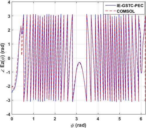
5.1. IE-GSTC-PEC validation example

To validate the formulation, consider the metasurface-PEC system example shown in Figure 13. The four metasurface segments are identical to what is shown in Table 1. The first quadrant in Table 1 corresponds to a metasurface segment in the range $0\le \varphi \le \pi /4$ in Figure 13 and so on. The dimensions are same as used in previous examples. The excitation is a plane wave ${\overline{E}}^{\mathrm{inc}}(x)=e^{-j{k}_{0}x}\hat{z}$. In Figures 14 and 15, IE-GSTC-PEC results are compared with COMSOL full wave simulations for fields on a circle of radius $10\lambda$.

Figure 13. Four segment metasurface with PEC backing.

This figure shows the metasurface with PEC segment which is used in validation example of Section 5. The upper half consists of 4 segments similar to previous examples and lower half is a PEC semi-circle.

Figure 14. IE-GSTC-PEC vs. full wave simulation results for four segment metasurface with PEC backing. $|E_z(\varphi )|$ vs. ϕ on a circle of radius 10λ.

This figure compares result of IE-GSTC-PEC example in Section 5 with results from commercially available CAD software COMSOL. The y-axis is the magnitude of z-component of electric field along a circle of radius 10 wavelengths. Good agreement between the two plots can be seen.

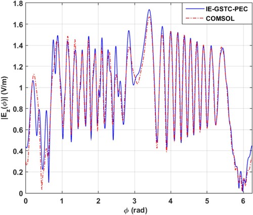
Figure 15. IE-GSTC-PEC vs. full wave simulation results for four segment metasurface with PEC backing. $\mathrm{\angle }{E}_z(\varphi )$ vs. ϕ on a circle of radius 10λ.

This figure compares result of IE-GSTC-PEC example in Section 5 with results from commercially available CAD software COMSOL. The y-axis is the phase of z-component of electric field along a circle of radius 10 wavelengths. Good agreement between the two plots can be seen.

6. Conclusion

This work validates IE-GSTC for circular cylindrical metasurfaces of nonzero thickness. The essence of this work is that physical circular metasurface scattering particles can be abstracted by a few numbers, i.e.susceptibility tensor components. To the author's knowledge, this work is one of the few works in which the GSTC and a bianisotropic susceptibility tensor model is validated for a physical, conformal metasurface. Although the examples and susceptibility extraction are presented for the TM polarization, they are easily extendable to the TE polarization. The combination can be used to analyze and design circular metasurfaces for the case of circularly polarized incident waves. This work is important in the sense that it pushes the previous works on conformal GSTC [10–12,14] to physical implementation and optimization. The IE-GSTC formulation is extended to handle PEC segments which could be useful for practical scattering reduction and radiation problems [29].

Disclosure statement

No potential conflict of interest was reported by the author(s).

Appendix. Multilayered magneto-dielectric shell inside a cylindrical surface electric current density

This section provides the analytical solution to the scattering problem shown in Figure 3. The excitation is a cylindrical surface electric current density of radius $a_s$, represented as ${\overline{J}}_s=\delta (\rho -a_s)\hat{z}$. Even though Figure 3 shows a three layered shell, this section generalizes it to m−1 magneto-dielectric layers. The m + 2 regions, i.e. m−1 magneto-dielectric regions, region internal to the shell, and space outside the shell separated into two regions by the surface current density are identified as follows: (A1) $\begin{array}{rl}& \mathrm{Region}i:a_{i-1}\le \rho \le a_i;i=1,2,\dots ,m+2\\ & a_0=0;a_{m+1}=a_s;a_{m+2}=\mathrm{\infty }\end{array}$(A1) where $a_{m+1}=a_s$ separates the external space (outside the magneto-dielectric shell) into two regions. There is a field discontinuity between these regions due to ${\overline{J}}_s=\delta (\rho -a_s)\hat{z}$. Region i has the constitutive parameters (${ϵ}_i,{\mu }_i$) and wave number $k_i=\omega \sqrt{{ϵ}_i{\mu }_i}$. Assuming no field or material variation along ϕ and z direction, the vector magnetic potential, electric field and magnetic field in each region for the case of $\mathrm{T}{\mathrm{M}}_{\mathrm{z}}$ polarization can be expressed in terms of Bessel functions. (A2a) $\begin{array}{rl}{A}_{z,i}\left(\rho \right)& =C_i{J}_0(k_i\rho )+D_i{Y}_0(k_i\rho )\end{array}$(A2a) (A2b) $\begin{array}{rl}{E}_{z,i}\left(\rho \right)& =-j\omega [C_i{J}_0(k_i\rho )+D_i{Y}_0(k_i\rho )]\end{array}$(A2b) (A2c) $\begin{array}{rl}{H}_{\varphi ,i}\left(\rho \right)& =\frac{k_i}{{\mu }_i}[C_i{J}_1(k_i\rho )+D_i{Y}_1(k_i\rho )]\end{array}$(A2c) where $J_0(\cdot ),Y_0(\cdot )$ are Bessel functions of the first and second kind, respectively. Hence there are $2(m+2)$ unknowns to be determined. The singularity of $Y_0(\cdot )$ at $\rho =0$ and the presence of only an outgoing wave in the outermost region m + 2, i.e. $A_{z,m+2}(\rho )\propto H_0^{(2)}(k_{m+2}\rho )$ entails the following conditions: (A3) $\begin{array}{rl}& D_1=0\\ & D_{m+2}+j{C}_{m+2}=0\end{array}$(A3) The continuity of the tangential electric field across the region interfaces results in: (A4) $\begin{array}{rl}& C_i{J}_0\left(k_i{a}_i\right)+D_i{Y}_0\left(k_i{a}_i\right)-C_{i+1}{J}_0\left(k_{i+1}{a}_i\right)\\ & -D_{i+1}{Y}_0\left(k_{i+1}{a}_{i+1}\right)=0;i=1,2,\dots ,m+1\end{array}$(A4) The continuity of the tangential magnetic field across the interfaces and the discontinuity caused by the surface electric current density excitation results in: (A5) $\begin{array}{rl}& C_i\frac{k_i}{{\mu }_i}{J}_1\left(k_i{a}_i\right)+D_i\frac{k_i}{{\mu }_i}{Y}_1\left(k_i{a}_i\right)-C_{i+1}\frac{k_{i+1}}{{\mu }_{i+1}}{J}_1\left(k_{i+1}{a}_i\right)\\ & -D_{i+1}\frac{k_{i+1}}{{\mu }_{i+1}}{Y}_1\left(k_{i+1}{a}_i\right)={\delta }_{i,m+1};i=1,2,\dots ,m+1\end{array}$(A5) The set of Equations (A3(A3) $\begin{array}{rl}& D_1=0\\ & D_{m+2}+j{C}_{m+2}=0\end{array}$(A3) ), (A4(A4) $\begin{array}{rl}& C_i{J}_0\left(k_i{a}_i\right)+D_i{Y}_0\left(k_i{a}_i\right)-C_{i+1}{J}_0\left(k_{i+1}{a}_i\right)\\ & -D_{i+1}{Y}_0\left(k_{i+1}{a}_{i+1}\right)=0;i=1,2,\dots ,m+1\end{array}$(A4) ) and (A5(A5) $\begin{array}{rl}& C_i\frac{k_i}{{\mu }_i}{J}_1\left(k_i{a}_i\right)+D_i\frac{k_i}{{\mu }_i}{Y}_1\left(k_i{a}_i\right)-C_{i+1}\frac{k_{i+1}}{{\mu }_{i+1}}{J}_1\left(k_{i+1}{a}_i\right)\\ & -D_{i+1}\frac{k_{i+1}}{{\mu }_{i+1}}{Y}_1\left(k_{i+1}{a}_i\right)={\delta }_{i,m+1};i=1,2,\dots ,m+1\end{array}$(A5) ) constitute $2(m+2)$ equations that can be solved for fields everywhere.

References

- Holloway CL, Kuester EF, Gordon JA, et al. An overview of the theory and applications of metasurfaces: the two-dimensional equivalents of metamaterials. IEEE Antennas Propag Mag. 2012 Apr;54(2):10–35. doi: 10.1109/MAP.2012.6230714
- Glybovski SB, Tretyakov SA, Belov PA, et al. Metasurfaces: from microwaves to visible. Phys Rep. 2016;634:1–72. doi: 10.1016/j.physrep.2016.04.004. Metasurfaces: From microwaves to visible.
- Yang F, Rahmat-Samii Y. Surface electromagnetics: with applications in antenna, microwave, and optical engineering. Cambridge University Press; 2019.
- Achouri K, Caloz C. Electromagnetic metasurfaces: theory and applications. John Wiley and Sons; 2021.
- Idemen M. Discontinuities in the electromagnetic field. 1st ed. John Wiley & Sons; 2011.
- Kuester EF, Mohamed MA, Piket-May M, et al. Averaged transition conditions for electromagnetic fields at a metafilm. IEEE Trans Antennas Propag. 2003;51(10):2641–2651. doi: 10.1109/TAP.2003.817560
- Achouri K, Salem MA, Caloz C. General metasurface synthesis based on susceptibility tensors. IEEE Trans Antennas Propagat. 2015;63(7):2977–2991. doi: 10.1109/TAP.2015.2423700
- Vahabzadeh Y, Achouri K, Caloz C. Simulation of metasurfaces in finite difference techniques. IEEE Trans Antennas Propag. 2016 Nov;64(11):4753–4759. doi: 10.1109/TAP.2016.2601347
- Sandeep S, Jin JM, Caloz C. Finite-element modeling of metasurfaces with generalized sheet transition conditions. IEEE Trans Antennas Propag. 2017 May;65(5):2413–2420. doi: 10.1109/TAP.2017.2679478
- Sandeep S, Huang SY. Simulation of circular cylindrical metasurfaces using GSTC-MOM. IEEE J Multiscale Multiphys Comput Tech. 2018;3:185–192. doi: 10.1109/JMMCT.2018.2881253
- Dehmollaian M, Chamanara N, Caloz C. Wave scattering by a cylindrical metasurface cavity of arbitrary cross section: theory and applications. IEEE Trans Antennas Propag. 2019;67(6):4059–4072. doi: 10.1109/TAP.8
- Dehmollaian M, Caloz C. Perfect penetrable cloaking using gain-less and loss-less bianisotropic metasurfaces. In: 2019 IEEE International Symposium on Antennas and Propagation and USNC-URSI Radio Science Meeting; 2019. p. 1323–1324.
- Safari M, Kazemi H, Abdolali A, et al. Illusion mechanisms with cylindrical metasurfaces: A general synthesis approach. Phys Rev B. 2019 Oct;100:Article ID 165418. doi: 10.1103/PhysRevB.100.165418
- Jia X, Vahabzadeh Y, Caloz C, et al. Synthesis of spherical metasurfaces based on susceptibility tensor gstcs. IEEE Trans Antennas Propag. 2019;67(4):2542–2554. doi: 10.1109/TAP.8
- Sandeep S, Huang SY. Fast analysis of spherical metasurfaces using vector wave function expansion. IEEE Antennas Wirel Propag Lett. 2019;18(6):1086–1090. doi: 10.1109/LAWP.7727
- Vellucci S, Monti A, Toscano A, et al. Scattering manipulation and camouflage of electrically small objects through metasurfaces. Phys Rev Appl. 2017 Mar;7:Article ID 034032. doi: 10.1103/PhysRevApplied.7.034032.
- Li H, Ma C, Shen F, et al. Wide-angle beam steering based on an active conformal metasurface lens. IEEE Access. 2019;7:185264–185272. doi: 10.1109/Access.6287639
- Xu G, Eleftheriades GV, Hum SV. Approach to the analysis and synthesis of cylindrical metasurfaces with noncircular cross sections based on conformal transformations. Phys Rev B. 2020 Dec;102:Article ID 245305. doi: 10.1103/PhysRevB.102.245305
- Xu G, Eleftheriades GV, Hum SV. Discrete-fourier-transform-based framework for analysis and synthesis of cylindrical Omega-bianisotropic metasurfaces. Phys Rev Appl. 2020 Dec;14:Article ID 064055. doi: 10.1103/PhysRevApplied.14.064055.
- Brown T, Narendra C, Vahabzadeh Y, et al. On the use of electromagnetic inversion for metasurface design. IEEE Trans Antennas Propag. 2020;68(3):1812–1824. doi: 10.1109/TAP.8
- Stewart S, de Jong YLC, Smy TJ, et al. Ray-optical evaluation of scattering from electrically large metasurfaces characterized by locally periodic surface susceptibilities. 2021. Available from: https://arxiv.org/abs/2102.07041.
- Lin CW, Grbic A. Analysis and synthesis of cascaded cylindrical metasurfaces using a wave matrix approach. IEEE Trans Antennas Propag. 2021;69(10):6546–6559. doi: 10.1109/TAP.2021.3070084
- Wang K, Zhang Q, Zhang Q. Electromagnetic simulation of 2.5-dimensional cylindrical metasurfaces with arbitrary shapes using gstc-mfcm. IEEE Access. 2020;8:142101–142110. doi: 10.1109/ACCESS.2020.3011835
- Stewart SA, Moslemi-Tabrizi S, Smy TJ, et al. Scattering field solutions of metasurfaces based on the boundary element method for interconnected regions in 2-d. IEEE Trans Antennas Propag. 2019;67(12):7487–7495. doi: 10.1109/TAP.8
- Smy TJ, Gupta S. Surface susceptibility synthesis of metasurface skins/holograms for electromagnetic camouflage/illusions. IEEE Access. 2020;8:226866–226886. doi: 10.1109/Access.6287639
- Jin JM. Theory and computation of electromagnetic fields. 2nd ed. Wiley-IEEE Press; 2015.
- Inan US, Marshall RA. Numerical electromagnetics–the fdtd method. Cambridge University Press; 2011.
- Dugan J, Smy TJ, Gupta S. Accelerated IE-GSTC solver for large-scale metasurface field scattering problems using fast multipole method (FMM). Techrxiv. 2021.
- Thtreswar B, Díaz-Rubio A, Asadchy V, et al. Step-wise homogeneous passive coatings for reduction of electromagnetic scattering from cylindrical metallic bodies. J Opt. 2020 Jul;22:Article ID 105601. doi: 10.1088/2040-8986/abaa62