Markov Models for Multi-state Language Change

ABSTRACT

Historical linguistics has witnessed an upsurge in quantitative corpus studies. The bulk of these studies involve the use of regression modelling. We point out a number of potential problems with this approach, and offer an alternative. For a multi-state language change, we propose a Markov model in continuous time. The major advantage of this technique, which has been used in medical contexts, is that it is especially geared towards dealing with time as a variable of interest, while it still allows one to look at the effect of several covariates. In this proof-of-concept article, we look at morphological shifts in preterites in Dutch, from 800ad to 2000ad (n = 14,314). This is a well-researched field, allowing us to investigate the performance of the multi-state Markov model.

1 Introduction

1.1 Inferential Statistics with the Variable Time

Recent decades have seen a drastic increase in the use of quantitative techniques in linguistics, to the extent that Janda (2013) speaks of ‘the quantitative turn’. Indeed, textbooks on quantitative methodology such as Baayen (2008a), Gries (2013), Levshina (2015), and Winter (2019) are among the best-selling in the field, and a bibliometric investigation of linguistic journals for the period 2005–2014 (Mohsen et al., 2017) revealed that the two most cited articles were decidedly quantitative in their approach and dealt with the application of mixed-models to the investigation of language (Baayen et al., 2008b; Jaeger, 2008). Though some subfields have been more reluctant in embracing this trend, hardly any subfield has remained completely untouched, and historical linguistics is no exception. Though historical linguistics has always relied on archival data (absent introspection as an easy access to facts), and early efforts to digitize such data can be counted as pioneering work (Hockey, 2004), full-blown integration of inferential statistic methods has advanced somewhat slower than in other subbranches of linguistics, if only because textual attestations are notoriously refractory and patchy. Labov famously quipped that “historical (…) can be thought of as the art of making the best use of bad data” (Labov, 1994, p. 11). Today, this has changed, and articles that make use of state-of-the-art methods are not hard to come by, see Hilpert and Gries (2016), Jenset and McGillivray (2017) and Van de Velde and Petré (2020) for overviews.

But what exactly are the state-of-the-art methods? While many techniques are in use, from simple significance tests (chi square, Fisher exact tests …) all the way to simulation studies (Baxter et al., 2009; Beuls & Steels, 2013; Blythe & Croft, 2012; Landsbergen et al., 2010; Lestrade, 2015; Nowak et al., 2001; Pijpops et al., 2015; Steels, 2016; Van Trijp, 2013), the main workhorse today is generalized linear (mixed)models, with time as an explanatory variable, often under multivariate control or in interaction with other covariates (see, a.o., De Cuypere, 2015; Fonteyn & Van de Pol, 2016; Gries & Hilpert, 2010; Petré & Van de Velde, 2018; Rosemeyer, 2016, 2014; Wolk et al., 2013; Zimmermann, 2017). This may seem reasonable, as regressing competing variants or frequency metrics on time can accommodate the typical S-curve that is observed in many cases of diachronic change (Blythe & Croft, 2012; Denison, 2003; Feltgen et al., 2017; Kroch, 1989; Pintzuk, 2003; Weinreich et al., 1968, p. 113).

While this approach appears to perform well, and can actually predict how the trajectory of a change proceeds, validated on a blinded part of the corpus (Van de Velde, 2017), they are, strictly speaking, in danger of giving too optimistic an image of the robustness of the model. The reason is that time is a peculiar variable, which does not exactly behave like other covariates entered in a multivariate model: ‘[T]he fact that time is a dynamic process provides challenges in formulating a model that are not present in settings where a typical linear or logistic regression model might be applied.’ (Hosmer et al., 2008, p. 2). One of the problems is that there is autocorrelation in the data, where consecutive time periods are not completely independent from one another, which can increase what in statistics is called Type I errors, by underestimating the standard error of the time variable (Cowpertwait & Metcalfe, 2009, p. 96). This can be solved in various ways. Baayen and Milin (2010) and De Smet and Van de Velde (2020a), for instance, apply a low-tech solution by adding the state of the outcome variable at a preceding time value as a covariate in the regression model. There is a burgeoning field of using methods which are specifically tailored to dealing with the temporal nature of the data, like time series analysis (Koplenig, 2017; Koplenig et al., 2016; Van de Velde & Petré, 2020), including Granger causality (Moscoso del Prado Martín, 2014; Rosemeyer & Van de Velde, 2020), and survival analysis (Van de Velde & Keersmaekers, 2020), a method widely applied in the medical sciences, engineering, and economics/sociology, where it is known as reliability analysis, duration analysis and event history analysis, respectively.

The purpose of the latter technique is to predict or model the time to an ‘event’, i.e. death of a patient, failure of a device etc. In linguistics, it can be used to assess lexical longevity, for instance, or to assess the time it takes for an incoming mutant to take over an old construction. In the latter case, the method is a viable competitor to generalized linear mixed models. By way of example, suppose we have two competing verbal suffixes (e.g. -μι vs. -ω for the 1sg.pres in Classical Greek, or -th vs. -s for the 3sg.pres in Early Modern English), and we want to model the increase of the second variant of such a pair, we could either regress the variants as a binary outcome variable on time and some other covariates (frequency of the verb, e.g.) and maybe add a random effect for verb, or we could use survival analysis and model the time to the event, in this case the switch to the new variant, depending on some covariate, using a typical method like a Cox Proportional Hazard model (see Hosmer et al., 2008, pp. 67–90; Harrell, 2015, pp. 427–436, 475–533, for mathematical and conceptual underpinnings). In the latter case, each verb is treated as a ‘patient’, if we look at it from a medical perspective.

1.2 Real-life Complications

As often in life, matters are usually more complicated. Several problems are likely to occur: (i) some verbs may disappear from the language before they had a change to trade in the old suffix for the new suffix, by a process of lexical replacement, or by just falling out of use. (ii) Maybe there is no real transition from an old variant to a new variant, but rather a ‘hesitant’ back-and-forth trajectory, depending on the verb. Even if the majority of changes show directionality, not all of them are on a conclusive path from an old A to a new B. Variation may be much more pervasive and functional than we might be inclined to assume (De Smet et al., 2018; Van de Velde, 2014; De Smet & Van de Velde, 2020b). (iii) Some verbs may be scantily attested and only appear at random times, so that we do not know exactly when it has changed its inflection in the meantime. We can only observe that when the verb surfaces in the textual record, it has either changed or not changed since the last time it was seen, and we are unsure about its behaviour when it dove under the waterline. (iv) Verbs may vary at a certain point in time, depending on the author, genre, register etc. This is especially likely in times of change.

Problem (i), lexical death, is not unknown in medical science, of course, where time to an event, say developing a pathology, can be blocked by a patient’s death. A naïve solution would be to treat these patients as ‘censored’, the technical term in survival analysis for patients that are lost to follow-up, because they fail to show up at consultation or because the observational study following patients stopped at a fixed point in time. This is standardly taken into account in survival analysis. But death of a patient is different. Unlike the censored patients, a deceased patient cannot develop the pathology any more. The solution is to build a model with what is technically called ‘competing risks’ or a ‘multi-state model’. Healthy patients can either become ill or die. Dealing with competing risks is a mathematical complication survival analysis is well-equipped to cope with (Putter et al., 2007).

Problem (ii), back-and-forth verb trajectories, is harder, both for a generalized linear (mixed) model and for simple survival analysis. In generalized linear (mixed) models, we expect a monotonous increase or decrease over time. Solutions have been offered, e.g. in the form of adding a quadratic term to deal with U-shaped change – the idea also underlies the approach known as ‘growth curve analysis’ – or with generalized additive (mixed) models (GAMMs), for even ‘wigglier’ curves (see Winter & Wieling, 2016). If the change is vacillating, with a lot of back-and-forth, the models will be quickly overparametrized. In survival analysis, the solution is extending the multi-state model such that recovery is possible from one state, but not from another.

Problem (iii), data scarcity for intermediate periods, is often glossed over in general linear (mixed) models, where it is customary to smoothen the curve between the observed datapoints. This involves reducing the residuals as much as possible, and designing a continuous function over time. The problem of potential change in the unseen time slices is hardly ever addressed. In survival analysis, the problem is acknowledged. In medical or sociological settings, the situation of problem (iii) is known as ‘panel data’ or ‘interval censoring’, and has an impact on the underlying analytical methods in survival analysis (Therneau et al., 2020a, p. 13, pp. 28–29).

Problem (iv), synchronic variation, is solved in general linear (mixed) models by allowing multiple datapoints at the same moment in time. In logistic regression with a binary outcome, the proportion of the two variants at a certain point in time can be accommodated by a binomial factor, with a weight for the number of observations. It is less straightforward to cope with this problem in survival analysis. A particular patient either has the disease or does not at a certain observation point. A patient is either dead or alive. A mechanical device either functions or fails. This is an underlying assumption of the models. This necessitates an idealization of discreteness of different stages in (continuous) time, see also Krylov (1995, pp. 19–20).

In short, general linear (mixed) models and survival analysis each have their advantages and drawbacks. The major drawback of the former is the overconfidence in the smoothness and monotonicity of the change, especially when there are gaps in the data, the major drawback of the latter is that it forces one to make a categorical decision about the state of the subject under investigation at a certain point in time. No single method is ideal. This echoes the words of the British statistician George Box: ‘All models are wrong; the practical question is how wrong do they have to be to not be useful.’

In this article, we will look at a well-studied linguistic change, which displays all problems (i)-(ii)-(iii)-(iv). We propose to use a multi-state Markov model. Because a lot is known about this particular change from extensive prior studies, we can validate the Markov model by confronting it with these earlier results. The change at issue is the preterite formation in Germanic. Our focus will be on Dutch.

2 Preterite Formation in Germanic

Ignoring the analytic perfect (ex. 1), which in some Germanic languages such as German, Dutch, and especially Afrikaans has been steadily gaining ground on the preterite for the past time reference (ex. 2 and 3), Germanic languages dispose of two ‘synthetic’ strategies to form the past. One is by changing the stem vowel (ex. 2), and the other is by adding a dental suffix (ex. 3). In historical linguistics, the former is called the ‘strong’ inflection, and is an Indo-European heirloom, while the latter is known as the ‘weak’ inflection, and is a Germanic innovation.¹

1. I have worked (analytic perfect)

2. drink ~ drank (strong preterite)

3. work ~ worked (weak preterite)

The distinction between the two inflection types is largely lexically specific: some verbs inflect strongly, other verbs inflect weakly. This distinction is, however, not diachronically stable. Through time, some weak verbs have become strong, but the more common ‘drift’ is for strong verbs to have become weak – understandably, as the weak inflection was originally the more innovative one, and is the default inflection for new verbs entering the system as loanwords. The gradual expansion of the weak inflection is a long-term change, spanning several hundred years. Historical linguistics have intensively studied these two competing morphological strategies for the Germanic preterite, both to reconstruct the earliest stages (i.a. Bailey, 1997; Hill, 2010; Lass, 1990; Mailhammer, 2007; Tops, 1974; Van Coetsem, 1990), and to trace the diachrony of the distribution (e.g. Anderwald, 2012; Cuskley et al., 2014 on 19^th-century English; Lieberman et al., 2007 on Old English to Present-day English, Carroll et al., 2012 on Old High German to Present-day German, De Vriendt, 1965 on 16^th-century Dutch; De Smet & Van de Velde, 2019, 2020a on 9^th-century to 20^th-century Dutch).

Of the quantitatively oriented studies, those which take a long term-perspective (> 1000 years, c.q. Carroll et al., 2012; De Smet & Van de Velde, 2019, 2020a; Lieberman et al., 2007), are invariably concerned with the major drift from strong to weak (or from irregular to regular), and do not take into account the reverse trajectory of verbs shifting (back) to the strong inflection, either temporarily or permanently. The number of (back)shifting verbs is, however, by no means marginal, at least not if we go by the figures in Cuskley et al. (2014) on Late Modern English.

Methodologically, this poses a challenge. If we would set up a binary logistic regression, with strong inflection vs. weak inflection as the outcome variable, the time coefficient might be zero when the two trends (strong-to-weak and weak-to-strong) cancel each other out, even if for some types of verbs, there may be a clear diachronic trend. Adding a quadratic term (e.g. $logit\left(P\left(weak\right)\right)={\beta }_0+{\beta }_{1}time+{\beta }_{2}tim{e}^2$), might alleviate the problem if the trend would turn out to be a U-shape, but it would underfit a more wavering trend. This is, in essence, problem (ii) referred to above. Problems (i) and (iii) are at play as well: verbs fall out of use in the course of time, and may hence cease to partake in the tug-of-war between the two inflectional types, and given the vast differences in token frequency, some verbs will regularly crop up in corpus studies, whereas others will only occasionally be witnessed. Problem (iv) manifests itself as well: for various synchronic slices, even if we take high-resolution snapshots per year, one and the same verb can occur both in the strong and in the weak inflection. Some linguistic studies amend this by setting a fixed value at a given time period (Carroll et al., 2012; De Smet & Van de Velde, 2019; Lieberman et al., 2007), which are derived by consulting reference grammars and dictionaries. Long-term large-scale corpus studies with higher resolution for variation (e.g. De Smet & Van de Velde, 2020a) are few and far between.

3 Methods and Data

3.1 Description of the Data

In this article, we will build a Markov model where, through time, verbs can either remain in the inflectional state they are in, or transition to an alternate state. One of the alternate states is lexical death. Though in principle, one can imagine a situation in which obsolete verbs are resurrected, we model this as a so-called ‘absorbing state’: once a verb crosses the Styx, there is no way back.

The first question is what the general lay-out of the Markov model should be here. Focusing on problem (ii), a simple transition diagram like Figure 1, which one would use in cases of binomial regression, is not suited. We need a more complicated diagram, like Figure 2, or, if we want to accommodate problem (i) as well, a diagram like Figure 3.

Figure 1. Transition diagram used in most binomial regression models.

Figure 2. Bidirectional transition diagram.

Figure 3. Bidirectional transitional diagram with lexical death (competing risks illness-death model with recovery).

The diagram in Figure 3 is well-known from the competing risks literature and is often called the illness-death model (Putter et al., 2007, p. 2414). The strong inflection can be compared to health, the weak inflection to illness, and lexical death to death. ‘Recovery’ from the illness state is possible, hence the double arrow between the strong and weak inflection.

We will feed this model with data for individual verbs, and see how likely it is that they transition to an alternate state over time. We took a large dataset, compiled for another study, consisting of all preterite and participle tokens of verbs which have been seen in the strong form in a corpus from the 9^th to the 20^th century, except for extremely frequent irregulars (zijn ‘be’, doen ‘do’, see ‘zien’, staan ‘stand’, gaan ‘go’, and worden ‘become’). We discarded the observations of the participles, retaining 189,841 observations of the preterites. These tokens represent 1630 different verb types, and 295 different verb stem types. With verb stems, we make abstraction of derivational-morphological operations: aanbieden (‘offer’), ontbieden (‘summon’) and bieden (‘offer’) are different verb types, but belong to the same stem. The observations were enriched for a large number of covariates. To keep things feasible, we will focus on two well-known covariates in this study, namely token frequency and the kind of vowel alternation pattern.

Frequency can be operationalized in a large number of ways (De Smet & Van de Velde, 2019), but we will enter it in the model as a ternary factor (‘low’, ‘medium’, and ‘high’), depending on whether the rounded base10 logarithm of the token frequency of the preterite of the stem was in the range 0 to 3, 4 to 6, or 6 to 10. Earlier studies have shown that the number of types is highest in the mid-range (a.o. Lieberman et al., 2007): low-frequency verbs tend to be weak, whereas high-frequency verbs do not count many members, due to the Zipfian distribution of words (Zipf, 1949). It is well-known that higher frequency verbs are less likely to change in inflection type.

Vowel pattern is also a ternary factor. Ablaut patterns come in different shapes, which are historically derived from 7 ablaut classes, but a major distinction is between so-called ABB, ABC and ABA verbs. ABB verbs have a distinct vowel in the present and the same vowel for the preterite and the participle (e.g. bijten /εɪ/ ~ beet /e:/ ~ gebeten /e:/, ‘bite’), ABC verbs have a distinct vowel in the present, past and participle (e.g. nemen /e:/ ~ nam /ɑ/ ~genomen /o:/, ‘take’), ABA verbs have the same vowel in the present and the participle, and a distinct vowel in the preterite (e.g. slapen /a:/ ~ sliep /i:/ ~ geslapen /a:/ ‘sleep’). Previous studies have shown that ABB preterites are best protected against weakening, because the distinct vowel in the present and the other two categories makes the ablaut more semiotically transparent, whereas ABA preterites are highly prone to change, because the vowel in the preterite works in isolation (De Smet & Van de Velde, 2019).

Not all of the observations in the dataset were useful for the present analysis. First, we discarded verbs that over time shifted from one of the 7 ablaut classes to another, because the vowel pattern may not be constant over time as well.² Survival analysis can accommodate working with time-dependent covariates (Therneau et al., 2020b), but this adds another layer of complexity, which we will refrain from in this study. Furthermore, we kept derivationally complex verbs in the dataset, unless they were compounds (bezighouden ‘keep busy’, flauwvallen ‘faint’, raadplegen ‘consult’ etc.). This left us with 184,761 preterite observations of 286 stems.

Then we had to make three additional assumptions; first, related to problem (iv) above, we retained just one instance per year per verb stem. This resulted in a serious reduction of the data, as a given text, from a given year, may contain numerous instances of the same verb. This is fairly straightforward if the verb is categorically weak or strong in a given year, but when there were both strong and weak forms in a given year, we had to decide. In such cases, we gave priority to the weak form, in line with earlier research (De Smet & Van de Velde, 2019, p. 156) (unless the minority form represented 10% or less of the extant forms in that particular year, in which case we assigned the majority form to the verb in that year), leaving us with 14,314 observations of 285 verbs stems.³ This is the second assumption. The idea is that weak forms will, on average be underestimated in the textual record, because they often represent the prescriptively dispreferred form. The obvious problem is that a single weak observation in a given year inbetween a sea of strong observations in adjacent time periods, will lead to a rapid transition in the Markov model. On the other hand, we do want to capture the erratic behaviour of preterite inflection. Note that most other studies also drastically reduce the variation to build statistical models (Carroll et al., 2012; De Smet & Van de Velde, 2019; Lieberman et al., 2007). Third assumption: we assumed a verb was dead if its stem was not observed in the last century anymore.⁴ In this case, we assumed the verb lived on for another generation after its last observation. A generation was taken to be 30 years. We used our native speaker knowledge to assess the quality of this filtering mechanism to check whether the verbs that experience lexical dead are indeed obsolete. This turned out to be the case. Verbs experiencing lexical death include dwaan (‘wash’), kweden (‘say’), zwelten (‘succumb’), a.o. (see Appendix B).

3.2 Under the Hood of the Multi-state Markov Model

The competing risk survival analysis technique used in this paper is known as a ‘multi-state Markov model in continuous time’ (Jackson, 2019). Like any inferential statistical technique it tries to infer an underlying, idealized picture (hence: ‘model’) from a set of discrete observations. This model can be used to extrapolate or predict reality beyond the observed data sample.

In Markov processes, the state of an individual or an object relies solely on its prior state, not on its history. A crucial notion in multi-state Markov models is the transitional intensity. As shown in Figure 3, various transitions are allowed, but not all transitions are equally likely. The intensity is the instantaneous risk that a verb will change from one state to the other, and can be captured by the following equation (Jackson, 2019, p. 2):

(4) $q_{rs}\left(t,Z\left(t\right)\right)=\underset{\mathrm{\Delta }t\to 0}{lim}\frac{P(S\left(t+\mathrm{\Delta }t\right)=s|S\left(t\right)=r)}{\mathrm{\Delta }t}$(4)

The transition intensity q for a pair of states r and s is a function of time t or a set of variables Z(t). These variables can be fixed at the level of the individual (in our model: the verb stem), or can be time-varying. As said above, we will limit ourselves to variables that remain constant for the individual and are known at the outset.

This transition intensity of state r to state s is defined as the limit of a time increment Δt as it goes to 0, of the probability of the assumed state S for an individual at time t+ Δt (which equals the probability of state s given that the assumed state at time t was state r) divided by Δt.

For each transition, a q can be calculated, which can be represented in the format of a matrix Q, in which the rows give the ‘from’ states and the columns the ‘to’ states. If 3 is the absorbing state (death), then we can substitute the last row with zeros. The diagonals are the negative of the sum of the other values at that row ($q_{rr}=-\sum _{r\ne s}{q}_{rs}$).

(5) $Q=\left(\begin{array}{c}{q}_{11}\\ q_{21}\\ q_{31}\end{array}\begin{array}{c}{q}_{12}\\ q_{22}\\ q_{32}\end{array}\begin{array}{c}{q}_{13}\\ q_{23}\\ q_{33}\end{array}\right)=\left(\begin{array}{c}-\left(q_{12}+q_{13}\right)\\ q_{21}\\ 0\end{array}\begin{array}{c}{q}_{12}\\ -\left(q_{21}+q_{23}\right)\\ 0\end{array}\begin{array}{c}{q}_{13}\\ q_{23}\\ -\left(q_{31}+q_{32}\right)=0\end{array}\right)$(5)

The transitional probabilities at time t involve exponentiating the scaled matrix Q (6), which involves solving a set of linear differential equations (see Cox & Miller, 1965 for details).

(6) $P\left(t\right)=e^{tQ}$(6)

(Time-independent) covariates are entered by multiplying a baseline $q_{rs}^0$ with an exponentiated covariate vector Z(t) multiplied by a coefficient β_rs.

(7) $q_{rs}\left(Z\left(t\right)\right)=q_{rs}^{baseline}{e}^{{\beta }_{rs}Z\left(t\right)}$(7)

The underlying assumption is that the effect of the covariate is proportional on the basis transition intensity. In that sense, it is reminiscent of a proportional hazard model, commonly used in survival analysis.

The likelihood function for the Maximum Likelihood Estimation of the multi-state Markov model can be found in Kalbfleisch and Lawless (1985). All calculations in this paper have been carried out with the package msm (Jackson, 2011) of the R software (R Core Team, 2019). For data wrangling we made use of the packages dplyr (Wickham et al., 2020) and reshape2 (Wickham, 2007).

4 Results

The model we will run has the transition intensities in (8) for r and s taking a value between 1 and 3, and with $q_{3s}=0$ for all 285 individual verb stems (see Appendix A). The model has two covariates frequency and vowel pattern, but as these are both ternary factors, we need 4 betas. Low-frequency range and ABB pattern are treated as reference levels.

(8) $q_{rs}\left(z\left(t\right)\right)=q_{rs}^{baseline}{e}^{\left({\beta }_{rs}^{mf}{Z}_{mf}\left(t\right)+{\beta }_{rs}^{hf}{Z}_{hf}\left(t\right)+{\beta }_{rs}^{ABC}{Z}_{ABC}\left(t\right)+{\beta }_{rs}^{ABA}{Z}_{ABA}\left(t\right)\right)}$(8)

(mf = mid-frequency, hf: high-frequency, ABC: vowel pattern ABC, ABA: vowel pattern ABA)

Before we run the model, let us first look at the descriptive statistics. The dataset contains information on 285 ‘individuals’, casu quo verb stems, together seen at non-set intervals – technically a kind of ‘non-informative sample times’ (Jackson, 2019, p. 4) – for a total number of 14,314 observations. Most of the times, verbs just stay in the state they were in before. So the bulk of the observations will be on the diagonal in the state table (Table 1).

Table 1. State table of the observations.

	to:
from:		strong	weak	dead
	strong	10741	265	38
	weak	240	3009	17
	dead	0	0	0

We can observe that transitions from strong to weak slightly outnumber the transition from weak to strong, but then again, there are more strong observations than weak observations in total.

Fitting the model with two covariates, frequency and vowel pattern yields the baseline transition intensities in Table 2.

Table 2. Baseline transition intensities.

transition	transition intensity	confidence interval
from strong to strong	−0.002	[−0.003, −0.002]
from strong to weak	0.002	[0.002, 0.003]
from strong to dead	<0.001	[<0.001, <1.000]
from weak to strong	0.008	[0.007, 0.010]
from weak to weak	−0.008	[−0.010, −0.007]
from weak to dead	<0.001	[0, ∞]

As in our dataset, verb stems are relatively unlikely to shift to the ‘dead’ state, the model has some trouble reliably calculating the transition intensities for transition to the ‘dead’ state (witness the large confidence intervals).⁵

Now let us turn to the effect of the covariates. Remember that these are expressed on the natural logarithm scale. Coefficients below 1 mean that the effect of the covariate is negative, lowering the transition intensity, and coefficients above 1 mean that the effect of the covariate is positive, boosting the transition intensity. The confidence interval should not span over the value 1.

For frequency, we can see that mid-frequency verbs have a lower probability to experience lexical death from either of the two states (strong or weak). For high-frequency verbs, the point estimates for the coefficient are even lower, but the confidence interval is too large to make the claim. Mid-frequency verbs have an increased probability of going from weak to strong, but not vice-versa. High-frequency verbs have a decreased probability to transition from strong to weak, but an increased probability to transition from weak to strong. Overall, this shows two things: first, the higher the frequency, the less likely the verbs shift to the weak inflection, a trend well-established in the literature, where frequency offers a protective effect against ‘regularization’ (Bybee, 2006, p. 715, who calls this the ‘conserving effect’). Second, that the higher the frequency of the verb, the more likely it shifts to the strong inflection state, if it was not already there. Here we concur with Fertig (2013, pp. 131–132), who argues that high-frequency verbs more easily undergo analogical, as opposed to regularization changes.

For the vowel pattern, we see that both ABC and ABA verbs are more likely to transition from strong to weak, and less likely to transition from weak to strong than ABB verbs. All this echoes the greater resilience to weakening found in ABB verbs (De Smet & Van de Velde, 2019), and the multi-state Markov model has the additional benefit that it shows that the latter effect not only transpires as ABB being protected to weakening but also a special proneness to shift back to the strong inflection, if it has slipped to the weak inflection.⁶ Lexical death is not significantly different in ABC or ABA verbs, compared to ABB verbs.

The model can also be used to calculate a transition probability matrix for specified durations. What is the probability of a verb stem to shift from strong to weak after 100 years, after 500 years, after 1000 years … taking into account the effects of the covariates? Tables 4–6 give the respective transition probability matrices. The higher the number of years, the less the figures change. The main trend is that verbs are more likely to transition from weak to strong, than from strong to weak. Again, this does not mean that verbs are massively turning into strong verbs, of course, as we only looked at verbs that belong to the strong group anywhere in their history. The high transition probabilities of weak-to-strong are mainly due to strong verbs getting back in line.

Table 3. Effect of the covariates Frequency (low-mid-high) and vowel pattern (ABB-ABC-ABA).

covariate		transition	coefficient	confidence interval
	low	(reference level)
frequency	mid	from strong to weak	1.06	[0.74, 1.54]
		from strong to dead	0.03	[0.01, 0.10]
		from weak to strong	2.38	[1.56, 3.64]
		from weak to dead	0.20	[0.06, 0.66]
	high	from strong to weak	0.37	[0.24, 0.57]
		from strong to dead	<0.01	[<0.01, >100.00]
		from weak to strong	2.52	[1.56, 4.08]
		from weak to dead	<0.01	[0.00, ∞]
vowel pattern	ABB	(reference level)
	ABC	from strong to weak	1.44	[1.00, 2.08]
		from strong to dead	1.31	[0.58, 2.93]
		from weak to strong	0.46	[0.32, 0.67]
		from weak to dead	0.34	[0.06, 1.99]
	ABA	from strong to weak	3.80	[2.86, 5.06]
		from strong to dead	0.93	[0.36, 2.41]
		from weak to strong	0.66	[0.49, 0.89]
		from weak to dead	0.76	[0.25, 2.32]

Table 4. Transition probability matrix for t = 100 (years).

	to:
from:		strong	weak	dead
	strong	0.861	0.139	<0.001
	weak	0.510	0.490	<0.001
	dead	0.000	0.000	1.000

Table 5. Transition probability matrix for t = 500 (years).

	to:
from:		strong	weak	dead
	strong	0.786	0.213	<0.001
	weak	0.781	0.219	<0.001
	dead	0.000	0.000	1.000

Table 6. Transition probability matrix for t = 1000 (years).

	to:
from:		strong	weak	dead
	strong	0.785	0.215	<0.001
	weak	0.785	0.215	<0.001
	dead	0.000	0.000	1.000

The next question we can ask is how long verbs stay in each state. This is technically known as the ‘sojourn time’. As can be appreciated from Table 7, the verbs in our dataset stay longer in the strong state than in the weak state:

Table 7. Sojourn times (in years).

	estimate	standard error	lower	upper
strong	445	36	379	522
weak	122	10	104	143

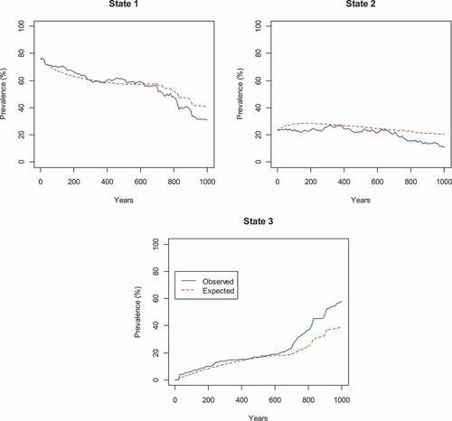
Model quality is visually assessed by comparing the observed and expected prevalence. In Figure 4, it is clear that the model becomes worse after 700 years, and starts to overestimate the prevalence in State 1 (strong) and State 2 (weak), and underestimate the prevalence in State 3 (dead), but otherwise the fit appears to be good.

Figure 4. Prevalence plots for ‘strong’ (State 1), ‘weak’ (State 2), and ‘dead’ (State 3).

5 Conclusion

In this article, we approached language change with a technique that does justice to the peculiar nature of the time variable. We built a multivariate multi-state Markov model in continuous time, which can be thought of as an offshoot of survival analysis. Over the past decades, such models have been applied in medical contexts, but so far, they have not often been tested against linguistic data. Krylov (1995) works out the mathematics of a model for semantic changes, but does not apply it to real data.

The advantage of this technique over more common techniques like generalized linear mixed models in which time is entered as a covariate, is that the Markov model can better capture the oscillation between different states. Unlike most generalized linear models it does not assume a monotonous linear, or S-shaped increase of decrease in two competing states, nor a U-shape. In this respect it can compete with generalized additive mixed models. The latter are data-hungry, and can lead to overfitting. Another advantage of the multi-state Markov Model is that it can work with competing risks.

This article is meant as a proof-of-concept. We build an illness-death model on Dutch preterite inflection, in which verbs can transition from the so-called ‘strong’ inflection to the so-called ‘weak’ inflection or vice versa, or experience lexical death. The results are compared with results from previous studies. Our Markov model seems to work well: it brings out the ‘conserving effect’, whereby frequency correlates with survival rates of a lexeme or a construction, and it brings out the protective effect of vowel patterns in the ablaut.

Disclosure statement

No potential conflict of interest was reported by the author(s).

Additional information

Funding

This work was supported by the FWO Vlaanderen [PhD 3H160540] and the Special Research Fund (BOF) from the University of Leuven [Project 3H180263 ‘How predictable is language change?’].

Notes

1. This terminology slightly deviates from the more familiar distinction between ‘regular verbs’, which predictably form their preterite with the suffix -ed, and the ‘irregular verbs’ (all the other verbs). The problem is that some irregular verbs are technically speaking weak (e.g. English keep – kept), and are irregular because of the influence of sound laws and analogy, and, conversely, that strong verbs are not devoid of regularity, as the specific vowel change (‘ablaut’) can be predicted from the present-tense vowel and the consonant skeleton of the root, especially in older languages stages and in Germanic languages other than English. This article is not the place to delve into the intricacies involved; readers are referred to historical reference grammars where these matters are explained in detail (e.g. Prokosch, 1939; Ringe, 2006), or to De Smet and Van de Velde (2019, pp. 141–143) for a concise discussion.

2. Occasionally, the vowel pattern of verbs that stay within their historical ablaut class also shifts diachronically. We followed the procedure in De Smet and Van de Velde (2019), and assigned one fixed value per verb.

3. We discarded one verb stem, fuiven (‘party’), which was only attested once in the dataset, and hence does not impact the Markov model.

4. We set the limit at 1914, the end of what historians call ‘the long 19^th century’.

5. We also ran a two-state model, without the death state (Figure 2, above), and this barely affected the baseline transition intensities (Table 2) or the covariate coefficients (Table 3, below). Future applications of the method tested in our proof-of-concept article would be well advised to use a phenomenon with higher death rates (lexical replacement). Here we stick to the three-state illness-death model. We adhere to the advice that model selection should be based on real-world or theoretical considerations, rather than deciding on the basis of statistical measures (see Harrell, 2015, pp. 67–72 in the context of regression).

6. As we have pointed out above, the dataset is biased towards weak verbs that became strong. The large number of verbs that happily stayed weak during their existence are not in our purview.

Appendix A.

Verb stem (types), observations per century (homonymous verbs disambiguated by English translation).

verb stem	century
	9	10	11	12	13	14	15	16	17	18	19	20
bakken	0	0	0	0	0	0	0	1	0	1	2	3
bannen	0	0	0	0	1	5	0	2	1	1	4	5
barsten	0	0	0	0	4	2	1	3	4	7	17	17
bassen	0	0	0	0	0	1	0	0	0	0	0	3
beiden	0	1	0	1	6	7	2	2	0	0	9	0
belgen	0	1	0	0	4	7	1	1	0	0	2	0
beren	0	1	0	1	2	4	5	4	11	5	7	4
bergen	0	0	0	0	1	4	7	4	4	9	17	17
beuren (‘heave’)	0	0	0	0	0	1	2	1	1	1	7	3
bidden	0	0	0	2	20	14	16	10	17	6	23	14
bieden	0	0	0	1	22	14	14	9	13	9	23	22
bijden	0	2	0	0	0	0	0	0	0	0	0	0
bijten	0	0	0	0	5	8	5	3	6	4	17	21
binden	0	0	0	0	13	10	8	3	7	8	18	17
blazen	0	0	0	0	6	0	0	1	3	1	5	21
blijken	0	0	0	0	1	1	3	5	12	8	17	25
blijven	0	1	0	1	28	16	17	12	23	20	24	30
blinken	0	0	0	0	0	0	1	0	5	7	17	11
blouwen	0	0	0	0	1	3	0	0	0	0	0	0
bouwen	0	0	0	0	0	0	1	4	2	3	10	13
braden	0	0	0	0	1	1	1	2	0	0	0	0
branden	0	0	0	0	7	9	12	5	8	8	19	21
breken	0	0	0	0	33	12	16	11	16	16	22	25
brouwen	0	0	0	0	0	1	0	1	1	1	0	2
bruiken	0	0	0	0	1	2	5	7	9	11	18	21
buigen	0	0	0	0	1	6	4	0	5	6	20	23
delven	0	0	0	0	1	1	0	1	0	2	1	4
derven	0	1	0	0	7	6	7	2	1	5	6	6
dijen	0	0	0	0	0	2	1	0	1	0	0	3
dingen	0	0	0	0	8	2	1	0	1	3	6	2
dinsen	0	1	0	0	2	0	0	0	0	0	0	0
draaien	0	0	0	0	1	2	0	2	6	5	15	24
draden	0	0	0	0	4	0	0	0	0	0	0	0
dragen	0	0	0	1	30	15	15	10	19	12	23	28
draven	0	0	0	0	0	1	0	0	0	1	8	8
drepen	0	0	2	0	0	0	0	0	0	0	0	0
driegen	0	0	0	1	4	4	4	3	2	5	14	7
drieten	0	0	0	0	1	6	7	2	4	1	5	3
drijven	0	0	1	0	8	10	10	8	13	9	23	19
dringen	0	0	0	1	1	6	1	3	7	8	20	21
drinken	0	0	1	0	9	13	11	5	10	6	22	26
druipen	0	0	1	0	0	0	0	1	4	3	9	12
duiken	0	0	0	0	1	0	0	1	2	3	8	15
duwen	0	1	0	0	2	1	0	1	3	3	11	20
dwaan	0	0	0	0	5	8	5	0	0	0	0	0
dwalen	0	0	0	0	0	0	3	2	3	4	15	14
dwijnen	0	0	0	0	0	0	0	4	7	5	20	21
dwingen	0	0	0	1	10	9	8	6	7	9	19	15
eisen	0	0	1	0	17	6	9	4	7	8	16	15
erven	0	0	0	0	14	5	0	0	0	2	4	2
eten	0	1	1	1	11	1	3	6	9	9	16	24
fijnen	0	0	0	0	0	5	0	0	0	0	0	0
fluiten	0	0	0	0	0	0	0	0	0	1	8	14
gelden	0	1	0	1	25	29	3	0	3	5	11	13
geten	0	0	0	2	7	8	8	5	4	8	22	21
geven	0	1	1	2	44	8	0	13	29	23	26	31
gieten	0	0	0	1	6	5	3	3	11	1	11	14
ginnen	0	0	0	1	9	12	12	6	18	15	24	32
glijden	0	0	0	0	1	0	1	0	3	2	14	19
glimmen	0	0	0	0	0	0	0	0	0	2	4	9
graven	0	1	0	0	4	9	6	2	5	4	7	12
grijnen	0	0	0	0	1	2	2	0	0	0	0	0
grijpen	0	0	1	1	7	10	10	7	9	13	23	26
grijzen	0	0	0	0	0	0	2	0	0	0	0	0
hangen	0	0	0	1	11	10	15	5	10	11	22	27
helen	0	1	0	1	1	4	1	3	1	1	4	2
helpen	0	0	0	1	13	12	10	3	12	8	22	24
heten	0	0	1	1	15	16	12	5	10	10	19	25
hijgen	0	0	0	0	0	0	0	0	2	1	11	15
hijsen	0	0	0	0	0	0	0	0	0	1	1	10
houden	0	0	0	0	34	21	15	12	19	19	24	31
houwen	0	1	0	0	3	6	2	1	2	3	3	0
jagen	0	0	0	0	13	6	8	6	9	6	18	20
kerven	0	0	0	0	0	0	0	0	0	1	1	1
kiezen	0	1	0	2	9	10	12	5	7	17	17	21
kijken	0	0	0	0	0	1	0	1	10	10	16	30
kijven	0	0	0	0	0	0	1	0	5	2	1	1
klagen	0	0	0	2	13	10	7	6	9	8	19	18
kleven	0	1	0	0	0	1	3	1	0	1	9	10
klieven	0	0	0	0	2	2	1	1	0	1	3	5
klijven	0	0	0	0	0	2	4	0	0	0	0	0
klimmen	0	0	0	0	5	9	13	4	9	9	22	21
klinken	0	0	0	0	0	5	1	0	3	5	20	27
klinken (‘hit’)	0	0	0	0	0	0	0	0	1	2	4	0
kluiven	0	0	0	0	0	0	0	1	0	2	0	0
knagen	0	0	0	0	0	1	0	2	0	3	5	3
kneden	0	0	0	0	0	0	0	0	0	0	1	4
knijpen	0	0	0	0	0	0	0	0	2	3	9	19
komen	0	1	1	2	46	31	16	17	32	23	26	33
kraaien	0	0	0	0	2	0	1	0	1	0	5	7
krijgen	0	0	0	0	18	9	10	11	26	22	22	33
krijsen	0	0	0	0	0	0	0	1	1	0	6	5
krijten	0	0	0	0	1	3	0	3	7	3	7	4
krimpen	0	0	0	0	2	1	0	0	1	2	5	13
kruien	0	0	0	0	0	1	1	0	2	0	0	0
kruipen	0	0	0	0	3	5	2	4	4	5	17	23
kruizen	0	0	0	0	0	0	0	0	2	0	0	0
kweden	0	1	0	2	0	0	0	0	0	0	0	0
kwelen	0	0	0	1	3	5	1	2	2	0	0	0
kwellen	0	0	0	0	2	3	2	6	4	3	11	5
kwijten	0	0	0	0	5	3	1	0	1	2	4	1
lachen	0	0	0	0	6	11	6	5	11	7	22	24
laden	0	0	0	0	4	7	2	0	0	2	9	9
laden (‘invite’)	0	0	0	0	0	2	0	0	0	0	0	0
laten	0	1	0	2	27	23	16	11	26	22	28	32
leggen	0	0	0	1	18	12	10	6	9	5	23	26
leiden	0	1	1	0	11	12	12	7	8	10	19	17
leken	0	0	0	0	3	2	1	0	0	1	1	2
lezen	0	0	0	0	9	10	10	5	9	11	21	29
liegen	0	0	0	1	6	8	7	4	2	3	5	9
liezen	0	0	0	1	15	11	13	5	10	11	20	22
liggen	0	0	1	1	23	15	13	11	27	17	25	30
lijden	0	1	1	2	11	17	13	2	15	10	21	17
lijden (‘declare’)	0	0	0	0	27	7	6	2	4	2	12	0
lijen (‘borrow’)	0	1	0	0	0	2	0	0	0	0	0	0
lijken	0	0	0	0	6	5	1	3	9	10	19	26
lijken (‘please’)	0	1	0	0	1	0	0	0	0	1	2	0
lopen	0	1	0	0	15	13	13	8	22	20	24	31
louwen	0	0	0	0	0	3	0	0	0	0	0	0
luiken	0	1	0	0	5	8	0	0	1	0	3	3
maaien	0	0	0	0	0	1	0	0	0	1	0	3
maken	0	1	1	1	30	16	15	13	23	14	23	32
malen	0	0	0	0	0	0	0	0	2	2	2	3
malen (‘paint’)	0	0	0	0	0	0	0	0	3	1	4	0
melken	0	0	0	0	0	0	1	0	0	0	0	1
meten	0	0	0	0	13	6	7	3	4	2	3	4
mijden	0	0	0	1	2	5	2	1	1	1	10	10
nemen	0	1	1	2	34	17	17	17	26	20	26	31
nezen	0	0	0	1	8	12	11	4	5	1	5	7
nieten	0	0	0	1	1	4	1	1	7	8	17	17
nijden	0	0	0	0	2	4	4	0	1	4	6	11
nijgen	0	0	0	0	4	6	2	0	1	1	3	3
nijpen	0	0	0	0	0	1	0	0	3	1	4	3
pijpen	0	0	0	0	0	0	0	0	3	0	0	0
pleken	0	0	0	0	0	2	0	0	0	0	0	0
pluiken	0	0	0	0	3	4	0	0	0	0	0	0
pluizen	0	0	0	0	0	0	0	0	0	0	0	2
prenden	0	0	0	0	2	3	2	0	0	0	0	0
prijzen	0	0	0	0	9	8	7	7	5	6	12	18
raden	0	0	1	2	11	6	5	7	10	8	19	14
reiken	0	0	0	0	1	2	1	1	2	6	24	23
reken	0	0	0	0	0	3	0	0	0	0	0	0
rekken	0	0	0	0	6	1	1	0	3	3	6	16
rijden	0	0	0	1	11	9	8	2	8	11	17	22
rijgen	0	0	0	0	0	0	0	0	1	0	4	0
rijnen	0	0	0	0	3	4	0	0	0	0	0	0
rijten	0	0	0	0	1	1	0	0	0	0	2	0
rijzen	0	0	0	0	2	8	9	5	11	8	20	14
rinnen	0	1	0	1	6	9	6	0	1	2	6	19
rispen	0	0	0	0	2	4	4	3	2	1	4	4
roepen	0	1	1	1	14	12	12	8	19	15	27	25
rouwen	0	0	0	0	5	4	2	2	1	0	7	2
ruiken	0	0	0	0	4	5	1	1	1	4	7	19
schaven	0	0	0	0	0	1	2	0	0	0	0	1
scheiden	0	1	0	1	15	14	9	4	8	4	18	16
schelden	0	1	0	0	30	6	5	2	4	7	10	11
schellen	0	1	0	0	0	0	0	0	1	0	11	2
schenden	0	0	0	0	2	3	0	1	1	3	4	1
schenken	0	0	0	0	3	3	7	4	9	9	23	19
scheppen	0	0	0	0	5	0	0	3	7	3	10	15
scheppen (‘create’)	0	0	0	1	2	6	7	4	9	6	8	9
scheren (‘order’)	0	0	0	0	5	0	0	0	0	2	0	0
schieden	0	0	1	1	18	13	12	6	15	10	11	11
schieten	0	0	0	0	9	9	10	5	12	10	21	24
schijnen	0	1	1	2	8	14	14	11	21	22	26	29
schijten	0	0	0	0	0	0	1	2	2	0	0	2
schrijden	0	0	0	0	1	2	2	1	1	0	4	17
schrijven	0	0	0	1	31	53	14	13	17	14	21	27
schrikken	0	0	0	0	0	0	0	3	8	7	19	23
schuilen	0	0	0	0	1	1	2	3	6	5	11	9
schuiven	0	0	0	0	0	3	0	0	4	7	17	22
seffen	0	0	0	1	1	6	1	1	2	2	9	15
slaan	0	1	1	1	25	13	15	10	23	16	23	27
slapen	0	1	0	0	8	8	8	4	9	8	22	23
slijpen	0	0	0	0	0	0	0	0	1	0	4	0
slijten	0	0	0	0	2	3	0	0	4	3	10	5
slinden	0	0	0	0	1	1	7	0	0	3	4	6
slinken	0	0	0	0	0	0	0	0	0	0	2	3
sluiken	0	0	0	0	0	0	0	0	2	0	0	0
sluipen	0	0	0	0	1	4	0	1	2	4	14	21
sluiten	0	0	0	0	3	10	11	8	12	18	24	29
smaden	0	0	0	0	2	3	9	2	1	3	5	2
smelten	0	0	0	0	2	5	0	2	4	3	11	10
smijten	0	0	0	0	0	4	1	3	7	4	10	13
snappen	0	0	0	0	0	0	0	1	3	3	15	17
snijden	0	0	1	0	8	7	10	4	10	4	16	15
snuiten	0	0	0	0	0	0	0	1	1	1	2	5
snuiven	0	0	0	0	0	0	0	0	0	1	4	12
spanen	0	0	0	0	0	5	1	0	0	0	0	0
spannen	0	0	0	0	2	5	4	1	4	5	16	15
spijten	0	0	0	0	0	0	0	4	6	6	14	11
spinnen	0	0	0	0	3	3	0	2	2	1	2	7
splijten	0	0	0	0	0	4	0	1	0	2	3	2
spreken	0	1	1	1	23	16	16	11	22	18	23	29
springen	0	0	0	0	8	9	8	5	10	9	21	25
spruiten	0	0	0	0	0	3	2	1	3	3	8	2
spugen	0	0	0	0	0	0	0	3	8	2	3	7
spuiten	0	0	0	0	0	0	0	0	1	0	1	6
stappen	0	0	0	0	2	2	0	0	2	7	20	24
stelen	0	0	0	0	6	5	2	3	6	1	8	3
stenen	0	0	0	0	0	3	1	0	1	0	5	0
sterven	0	0	1	1	26	20	16	9	16	15	21	18
stijgen	0	1	0	0	0	0	1	1	7	6	19	20
stijven	0	0	0	0	0	0	0	0	2	2	3	8
stinken	0	0	0	0	1	2	2	2	3	2	1	7
stoten	0	0	0	1	7	7	5	4	11	5	17	18
strijden	0	0	0	0	4	12	9	5	6	7	15	16
strijken	0	0	1	0	10	9	6	3	8	1	16	21
stuipen	0	0	0	0	0	1	2	0	0	0	0	0
stuiten	0	0	0	0	0	0	0	1	0	1	8	8
stuiven	0	0	0	0	1	2	2	0	3	4	13	16
tamen	0	0	0	2	6	7	5	4	3	0	5	1
tijgen	0	0	0	1	4	9	14	2	10	6	13	6
tijgen (‘accuse’)	0	0	0	0	15	8	6	1	1	0	2	0
treffen	0	0	0	0	0	0	0	1	9	12	23	22
trekken	0	0	0	0	18	13	8	8	21	16	26	29
vallen	0	1	0	2	30	24	15	13	25	19	26	31
vangen	0	1	1	2	29	14	10	5	12	8	23	22
varen	0	1	0	0	20	18	12	4	16	14	20	21
vechten	0	0	1	2	10	10	8	3	4	6	6	12
velen	0	0	0	1	10	11	13	10	4	5	15	11
vijsten	0	0	0	0	0	0	0	0	2	0	0	0
vinden	0	1	1	2	29	21	16	13	28	21	27	32
vlechten	0	0	0	0	3	0	1	0	1	1	3	3
vlieden	0	0	0	0	10	8	11	6	7	3	13	2
vliegen	0	0	0	0	6	9	8	7	13	12	22	26
vlieten	1	0	0	0	3	5	1	1	4	1	4	0
vlijen	0	0	0	0	0	0	0	0	1	2	7	7
vlijten	0	0	0	2	0	0	0	0	0	0	0	0
vloeken	0	1	0	0	2	3	2	2	9	5	9	16
vouwen	0	0	0	0	5	0	1	2	0	1	17	16
vragen	0	0	0	0	10	12	15	7	14	15	22	31
vreisen	0	0	0	1	0	3	0	0	0	0	0	0
vreten	0	0	0	0	0	1	0	1	5	3	1	12
vriezen	0	0	0	0	1	2	1	1	3	1	2	3
vrijen	0	0	0	0	0	0	2	0	5	3	4	1
waaien	0	0	0	0	3	2	2	2	3	2	15	14
waden	0	0	0	0	4	5	2	0	0	0	1	3
wagen	0	0	0	1	4	3	1	0	2	0	5	1
waken	0	0	0	0	6	8	4	2	7	8	19	15
wallen	0	1	0	0	2	2	2	0	0	0	0	0
warren	0	0	0	0	3	3	1	1	1	2	2	6
wassen (‘grow’)	0	0	0	0	4	11	9	4	4	3	3	2
waten	0	2	0	0	0	0	0	0	0	0	0	0
wellen	0	1	2	0	0	0	0	0	0	0	0	0
werpen	0	1	1	0	18	12	13	7	6	9	22	22
werven	0	0	0	2	3	7	7	2	3	2	9	7
weven	0	0	0	0	5	0	0	0	0	1	2	4
wijken	0	0	0	0	2	2	1	2	7	8	18	18
wijten	0	1	0	0	4	7	5	3	4	5	14	5
wijzen	0	0	1	0	30	10	9	8	13	11	24	24
winden	0	0	0	1	9	7	8	2	1	6	9	11
winnen	0	0	1	1	19	13	14	5	15	14	18	17
woepen	0	2	0	0	0	0	0	0	0	0	0	0
wouden	0	1	0	0	1	4	5	0	0	0	0	0
wreken	0	0	0	0	3	6	4	0	1	1	5	2
wrijven	0	0	0	0	2	3	2	2	4	3	12	14
wringen	0	0	0	0	1	4	1	1	0	0	1	15
wuiven	0	0	0	0	0	2	0	0	0	1	11	20
zaaien	0	0	0	0	2	3	2	0	2	3	4	3
zaken	0	0	0	1	1	2	2	0	3	3	2	1
zenden	0	1	0	2	16	13	14	8	17	17	20	18
zetten	0	1	1	1	29	13	15	3	8	9	23	27
zieden	0	0	0	0	2	2	1	0	0	0	1	4
zijgen	0	0	0	0	2	3	0	0	2	2	10	6
zijken	0	0	0	0	0	4	0	0	0	0	0	0
zijpen	0	0	0	0	2	0	0	0	0	0	0	0
zingen	0	1	0	1	8	7	11	2	11	7	15	16
zinken	0	0	0	0	5	6	4	4	5	3	21	4
zinnen	0	0	0	1	0	4	2	2	4	3	6	9
zitten	0	1	1	1	17	12	14	11	22	18	26	32
zouten	0	0	0	0	3	0	2	0	0	0	0	0
zuigen	0	0	0	0	2	4	2	0	4	0	2	12
zuipen	0	0	0	0	0	1	0	0	1	2	1	3
zwelgen	0	0	0	0	2	1	1	1	2	0	3	1
zwellen	0	0	0	0	1	2	0	0	1	1	5	9
zwelten	0	0	0	0	0	3	0	0	0	0	0	0
zwemmen	0	0	0	0	1	2	3	1	6	2	8	13
zweren	0	0	1	1	16	7	10	5	12	9	11	12
zweren (‘fester’)	0	0	0	0	0	2	1	1	1	0	0	1
zwerven	0	0	0	0	0	0	0	1	1	2	10	6
zwijgen	0	0	0	0	7	8	6	5	9	8	20	20
zwijken	0	0	0	0	1	3	0	0	4	2	2	7
zwinden	0	0	0	0	0	1	0	0	0	1	1	1
zwingen	0	0	0	0	0	1	2	2	0	0	0	0

Appendix B.

verb stems experiencing lexical death (last seen before or in 1914)

beiden, belgen, bijden, blouwen, braden, dinsen, draden, drepen, dwaan, fijnen, grijnen, grijzen, houwen, klijven, klinken (‘hit’), kluiven, kruien, kruizen, kweden, kwelen, laden (‘invite’), lijden (‘declare’), lijen (‘borrow’), lijken (‘please’), louwen, malen (‘paint’), pijpen, pleken, pluiken, prenden, reken, rijgen, rijnen, rijten, scheren (‘arrange’), slijpen, sluiken, spanen, stenen, stuipen, tijgen (‘accuse’), vijsten, vlieten, vlijten, vreisen, wallen, waten, wellen, woepen, wouden, zijken, zijpen, zouten, zwelten, zwingen

(Homonymous verbs disambiguated by English translation)

References

- Anderwald, L. (2012). Variable past tense forms in 19th-century American English: Linking normative grammars and language change. American Speech, 87(3), 257–293. https://doi.org/https://doi.org/10.1215/00031283-1958327
- Baayen, R. H. (2008a). Analyzing linguistic data: A practical introduction to statistics using R. Cambridge University Press.
- Baayen, R. H., Davidson, D. J., & Bates, D. M. (2008b). Mixed-effects modeling with crossed random effects for subjects and items. Journal of Memory and Language, 59(4), 390–412. https://doi.org/https://doi.org/10.1016/j.jml.2007.12.005
- Baayen, R. H., & Milin, P. (2010). Analyzing reaction times. International Journal of Psychological Research, 3(2), 12–28. https://doi.org/https://doi.org/10.21500/20112084.807
- Bailey, C. G. (1997). The etymology of the old high German weak verb [PhD Diss]. Newcastle upon Tyne.
- Baxter, G. J., Blythe, R. A., Croft, W., & McKane, A. J. (2009). Modeling language change: An evaluation of Trudgill’s theory of the emergence of New Zealand English. Language Variation and Change, 21(2), 257–296. https://doi.org/https://doi.org/10.1017/S095439450999010X
- Beuls, K., & Steels, L. (2013). Agent-based models of strategies for the emergence and evolution of grammatical agreement. PLoS ONE, 8(3), e58960. https://doi.org/https://doi.org/10.1371/journal.pone.0058960
- Blythe, R. A., & Croft, W. (2012). S-curves and the mechanisms of propagation in language change. Language, 88(2), 269–304. https://doi.org/https://doi.org/10.1353/lan.2012.0027
- Bybee, J. (2006). From usage to grammar: The mind’s response to repetition. Language, 82(4), 711–733. https://doi.org/https://doi.org/10.1353/lan.2006.0186
- Carroll, R., Svare, R., & Salmons, J. (2012). Quantifying the evolutionary dynamics of German verbs. Journal of Historical Linguistics, 2(2), 153–172. https://doi.org/https://doi.org/10.1075/jhl.2.2.01car
- Cowpertwait, P. S. P., & Metcalfe, A. V. (2009). Introductory time series with R. Springer.
- Cox, D. R., & Miller, H. D. (1965). The theory of stochastic processes. Chapman & Hall.
- Cuskley, C., Pugliese, M., Castellano, C., Colaiori, F., Loreto, V., & Tria, F. (2014). Internal and external dynamics in language: Evidence from verb regularity in a historical corpus of English. PLoS ONE, 9(8), e102882. https://doi.org/https://doi.org/10.1371/journal.pone.0102882
- De Cuypere, L. (2015). The Old English to-dative construction. English Language and Linguistics, 19(1), 1–26. https://doi.org/https://doi.org/10.1017/S1360674314000276
- De Smet, H., Fonteyn, L., D’hoedt, F., & Van Goethem, K. (2018). The changing functions of competing forms: Attraction and differentiation. Cognitive Linguistics, 29(2), 197–234. https://doi.org/https://doi.org/10.1515/cog-2016-0025
- De Smet, I., & Van de Velde, F. (2019). Reassessing the evolution of West-Germanic preterite inflection. Diachronica, 36(2), 139–179. https://doi.org/https://doi.org/10.1075/dia.18020.des
- De Smet, I., & Van de Velde, F. (2020a). A corpus-based quantitative analysis of twelve centuries of preterite and past participle morphology in Dutch. Language Variation and Change, 32(2), 241–265. https://doi.org/https://doi.org/10.1017/S0954394520000101
- De Smet, I. & Van de Velde, F. (2020b). Semantic differences between strong and weak verb forms in Dutch. Cognitive Linguistics, 31(3), 393–416
- De Vriendt, S. F. L. (1965). Sterke werkwoorden en sterke werkwoordsvormen in de 16de eeuw. Belgisch interuniversitair centrum voor neerlandistiek.
- Denison, D. (2003). Log(ist)ic and simplistic S-curves. In R. Hickey (Ed.), Motives for language change (pp. 54–70). Cambridge University Press.
- Feltgen, Q., Fagard, B., & Nadal, J. P. (2017). Frequency patterns of semantic change: Corpus-based evidence of a near-critical dynamics in language change. Royal Society Open Science, 4(11), 170830. https://doi.org/https://doi.org/10.1098/rsos.170830
- Fertig, D. (2013). Analogy and morphological change. Edinburgh University Press.
- Fonteyn, L., & Van de Pol, N. (2016). Divide and conquer: The formation and functional dynamics of the modern English ing-clause network. English Language and Linguistics, 20(2), 185–219. https://doi.org/https://doi.org/10.1017/S1360674315000258
- Gries, S. T. (2013). Statistics for linguistics with R. A practical introduction (2nd ed.). De Gruyter.
- Gries, S. T., & Hilpert, M. (2010). Modeling diachronic change in the third person singular: A multi-factorial, verb- and author-specific exploratory approach. English Language and Linguistics, 14(3), 293–320. https://doi.org/https://doi.org/10.1017/S1360674310000092
- Harrell, F. E., Jr. (2015). Regression modeling. Strategies with applications to linear models, logistic and ordinal regression, and survival analysis (2nd ed.). Springer.
- Hill, E. (2010). A case study in grammaticalized inflectional morphology: Origin and development of the Germanic weak preterite. Diachronica, 27(3), 411–458. https://doi.org/https://doi.org/10.1075/dia.27.3.02hil
- Hilpert, M., & Gries, S. T. (2016). Quantitative approaches to diachronic corpus linguistics. In M. Kytö & P. Pahta (Eds.), The Cambridge handbook of English historical linguistics (pp. 36–53). Cambridge University Press.
- Hockey, S. (2004). The history of humanities computing. In S. Schreibman, R. Siemens, & J. Unsworth (Eds.), A companion to digital humanities (pp. 3–19). Blackwell.
- Hosmer, D. W., Lemeshow, S., & May, S. (2008). Applied survival analysis: Regression modeling of time‐to‐event data (2nd ed.). John Wiley.
- Jackson, C. H. (2011). Multi-state models for panel data: The msm package for R. Journal of Statistical Software, 38(8), 1–29. https://doi.org/https://doi.org/10.18637/jss.v038.i08
- Jackson, C. H. (2019). Multi-state modelling with R: The msm package. Version 1.6.8. https://cran.r-project.org/web/packages/msm/vignettes/msm-manual.pdf
- Jaeger, T. F. (2008). Categorical data analysis: Away from ANOVAs (transformation or not) and towards logit mixed models. Journal of Memory and Language, 59(4), 434–446. https://doi.org/https://doi.org/10.1016/j.jml.2007.11.007
- Janda, L. A. (ed.). (2013). Cognitive linguistics – The quantitative turn. The essential reader. Mouton de Gruyter.
- Jenset, G. B., & McGillivray, B. (2017). Quantitative historical linguistics. A corpus framework. Oxford University Press.
- Kalbfleisch, J. D., & Lawless, J. F. (1985). The analysis of panel data under a Markov assumption. Journal of the American Statistical Association, 80(392), 863–871. https://doi.org/https://doi.org/10.1080/01621459.1985.10478195
- Koplenig, A. (2017). Why the quantitative analysis of diachronic corpora that does not consider the temporal aspect of time-series can lead to wrong conclusions. Digital Scholarship in the Humanities, 32(1), 159–168. https://doi.org/https://doi.org/10.1093/llc/fqv030
- Koplenig, A., Müller-Spitzer, C., & Lidzba, K. (2016). Population size predicts lexical diversity, but so does the mean sea level – Why it is important to correctly account for the structure of temporal data. PLoS ONE, 11(3), e0150771. https://doi.org/https://doi.org/10.1371/journal.pone.0150771
- Kroch, A. (1989). Reflexes of grammar in patterns of language change. Language Variation and Change, 1(3), 199–244. https://doi.org/https://doi.org/10.1017/S0954394500000168
- Krylov, Y. K. (1995). A Markov model for the evolution of lexical ambiguity. Journal of Quantitative Linguistics, 2(1), 19–26. https://doi.org/https://doi.org/10.1080/09296179508590031
- Labov, W. (1994). Principles of linguistic change, vol. 1: Internal factors. Blackwell.
- Landsbergen, F., Lachlan, R., ten Cate, C., & Verhagen, A. (2010). A cultural evolutionary model of patterns in semantic change. Linguistics, 48(2), 363–390. https://doi.org/https://doi.org/10.1515/ling.2010.012
- Lass, R. (1990). How to do things with junk: Exaptation in language evolution. Journal of Linguistics, 26(1), 79–102. https://doi.org/https://doi.org/10.1017/S0022226700014432
- Lestrade, S. (2015). A case of cultural evolution: The emergence of morphological case. In B. Köhnlein & J. Audring (Eds.), Linguistics in the Netherlands (pp. 105–115). John Benjamins.
- Levshina, N. (2015). How to do linguistics with R: Data exploration and statistical analysis. John Benjamins.
- Lieberman, E., Michel, J.-B., Jackson, J., Tang, T., & Nowak, M. A. (2007). Quantifying the evolutionary dynamics of language. Nature, 449(7163), 713–716. https://doi.org/https://doi.org/10.1038/nature06137
- Mailhammer, R. (2007). The Germanic strong verbs: Foundations and development of a new system. Mouton De Gruyter.
- Mohsen, M. A., Fu, H.-Z., & Ho, Y.-S. (2017). A bibliometric analysis of linguistics publications in the web of science. Journal of Scientometric Research, 6(2), 115–124. https://doi.org/https://doi.org/10.5530/jscires.6.2.16
- Moscoso del Prado Martín, F. (2014). Grammatical change begins within the word: Causal modeling of the co-evolution of Icelandic morphology and syntax. Proceedings of the Annual Meeting of the Cognitive Science Society, 36, 2657–2662.
- Nowak, M. A., Komarova, N. L., & Niyogi, P. (2001). Evolution of universal grammar. Science, 291(5501), 114–118. https://doi.org/https://doi.org/10.1126/science.291.5501.114
- Petré, P., & Van de Velde, F. (2018). The real-time dynamics of the individual and the community in grammaticalization. Language, 94(4), 867–901. https://doi.org/https://doi.org/10.1353/lan.2018.0056
- Pijpops, D., Beuls, K., & Van de Velde, F. (2015). The rise of the verbal weak inflection in Germanic. An agent-based model. Computational Linguistics in the Netherlands Journal, 5, 81–102.
- Pintzuk, S. (2003). Variationist approaches to syntactic change. In B. Joseph & R. Janda (Eds.), The handbook of historical linguistics (pp. 509–528). Blackwell.
- Prokosch, E. (1939). A comparative Germanic grammar. Linguistic Society of America.
- Putter, H., Fiocco, M., & Geskus, R. B. (2007). Tutorial in biostatistics: Competing risks and multi-state models. Statistics in Medicine, 26(11), 2389–2430. https://doi.org/https://doi.org/10.1002/sim.2712
- R Core Team. (2019). R: A language and environment for statistical computing. Foundation for Statistical Computing. https://www.R-project.org/.
- Ringe, D. (2006). From Proto-Indo-European to Proto-Germanic. Oxford University Press.
- Rosemeyer, M. (2014). Auxiliary selection in Spanish. Gradience, gradualness, and conservation. Studies in language companion series. Benjamins.
- Rosemeyer, M. (2016). Modeling frequency effects in language change. In H. Behrens & S. Pfänder (Eds.), Experience counts: Frequency effects in language (pp. 175–207). De Gruyter.
- Rosemeyer, M., & Van de Velde, F. (2020). On cause and correlation in language change. Word order and clefting in Brazilian Portuguese. Language Dynamics and Change, 10. https://doi.org/https://doi.org/10.1163/22105832-01001500)
- Steels, L. (2016). Agent-based models for the emergence and evolution of grammar. Philosophical Transactions of the Royal Society B, 371(1701), 20150447. https://doi.org/https://doi.org/10.1098/rstb.2015.0447
- Therneau, T., Crowson, C., & Atkinson, E. 2020a. ‘Multi-state models and competing risks’. https://cran.r-project.org/web/packages/survival/vignettes/compete.pdf.
- Therneau, T., Crowson, C., & Atkinson, E. 2020b. ‘Using time dependent covariates and time dependent coefficients in the Cox model’. https://cran.r-project.org/web/packages/survival/vignettes/timedep.pdf.
- Tops, G. A. J. (1974). The origin of the Germanic dental preterit. Brill.
- Van Coetsem, F. (1990). Ablaut and the reduplication in the Germanic verb. Carl Winter.
- Van de Velde, F. (2014). Degeneracy: The maintenance of constructional networks. In R. Boogaart, T. Colleman, & G. Rutten (Eds.), The extending scope of construction grammar (pp. 141–179). De Gruyter Mouton.
- Van de Velde, F. (2017). Understanding grammar at the community level requires a diachronic perspective. Evidence from four case studies. Nederlandse Taalkunde, 22(1), 47–74. https://doi.org/https://doi.org/10.5117/NEDTAA2017.1.VELD
- Van de Velde, F., & Keersmaekers, A. (2020). What are the determinants of survival curves of words? An evolutionary linguistics approach. Evolutionary Linguistic Theory, 2(2), 127–137.
- Van de Velde, F., & Petré, P. (2020). Historical linguistics. In D. Knight & S. Adolphs (Eds.), The Routledge handbook of English language and digital humanities (pp. 328–359). Routledge.
- Van Trijp, R. (2013). Linguistic selection criteria for explaining language change: A case study on syncretism in German definite articles. Language Dynamics and Change, 3(1), 105–132. https://doi.org/https://doi.org/10.1163/22105832-13030106
- Weinreich, U., Labov, W., & Herzog, M. (1968). Empirical foundations for a theory of language change. In W. Lehmann & Y. Malkiel (Eds.), Directions for historical linguistics (pp. 95–188). University of Texas Press.
- Wickham, H. (2007). Reshaping data with the reshape package. Journal of Statistical Software, 21(12), 1–20. https://doi.org/https://doi.org/10.18637/jss.v021.i12
- Wickham, H., Romain, F., Henry, L., & Müller, K. (2020). dplyr: A grammar of data manipulation. R package version 0.8.4.
- Winter, B. (2019). Applied statistics for linguists: An introduction using R. Routledge.
- Winter, B., & Wieling, M. (2016). How to analyze linguistic change using mixed models, growth curve analysis and generalized additive modeling. Journal of Language Evolution, 1(1), 7–18. https://doi.org/https://doi.org/10.1093/jole/lzv003
- Wolk, C., Bresnan, J., Rosenbach, A., & Szmrecsanyi, B. (2013). Dative and genitive variability in late modern English: Exploring cross-constructional variation and change. Diachronica, 30(3), 382–419. https://doi.org/https://doi.org/10.1075/dia.30.3.04wol
- Zimmermann, R. (2017). Formal and quantitative approaches to the study of syntactic change: Three case studies from the history of English [PhD Diss.]. Université de Genève.
- Zipf, G. K. (1949). Human behavior and the principle of least effort. An introduction to human ecology. Addison-Wesley Press.