Theory and practice of higher-order frequency modulation synthesis

Abstract

Frequency modulation (FM) and phase modulation (PM) are well-known synthesis methods, which have been deployed widely in musical instruments. In this paper, we analyse the design of stacked FM synthesis and using a direct comparison with PM, put forward a method we call higher-order frequency modulation (hoFM). We begin by reviewing the theory of first-order FM, contrasting it to PM. We then discuss the problems of extending first-order FM by simply applying the modulation to the frequency, which may result in carrier drift caused by the presence of DC in the modulating signal. We proceed to develop a formulation of second-order FM which is equivalent to the issue-free PM synthesis, and present an expression for the evaluation of the second-order FM spectrum. By virtue of the application of amplitude modulation concurrently with frequency modulation, we are able to eliminate the DC component and thus any carrier drift caused by it. These principles are then extended to higher-order topologies, where we note that in the general case, the modulation signal at each level is amplitude modulated by its own FM input. From this, we are able to advance the concept of an FM operator, analogous to the one used in PM instrument design, to realise hoFM. From this we demonstrate that feedback FM is also a practical possibility. Finally, moving from continuous to discrete time, we develop a reference C++ implementation for computer music applications, and discuss issues relating to digital implementations.

Keywords:

• Sound synthesis
• non-linear distortion
• frequency modulation
• phase modulation
• feedback

1. Introduction

Linear frequency modulation (FM) as a sound synthesis technique has had a long history of development, first explored by James Tenney, followed by Jean-Claude Risset and John Chowning (Lazzarini et al., 2023). It was given a theoretical treatment by Chowning (1973), where he demonstrated it could provide an economical method of producing dynamic spectra with both harmonic and inharmonic partials. FM was also shown to generate sounds previously only possible with the more computationally expensive means of additive synthesis. Through the similar, but more flexible form of phase modulation (PM), which was the actual object of analysis in Chowning's paper, the method was implemented in a very successful range of digital synthesisers, first by Yamaha (Chowning & Bristow, 1986), then by other vendors. In this form it was expanded to support higher-order (or stacked) as well as feedback modulation. Both extensions can be characterised as forms of complex (as in multi-component) PM.

The mathematical formulation of FM and PM is generally accepted to stem from the early studies in radio frequency broadcasting (Bloch, 1944; Corrington, 1947), but in fact its roots extend further back to John Bernoulli in 1694 (Watson, 1944, p. 1). The concept of an instantaneous frequency, as the time derivative of the phase angle, was first introduced in order to support the development of such modulation theory (Carson, 1922), and since Gabor (1940) it has become a cornerstone of modern spectral audio theory (Lazzarini, 2021). In these early papers, the exact distinction between the two forms of modulation was not a concern for the authors, as the principles being developed could be implemented with either one of the methods. However, it is important to note that most of the mathematics underpinning these ideas, arising from the theory of Bessel coefficients, applies first and foremost to PM and only in a second instance to FM, as we will show in this paper.

The subject of PM has been studied extensively since Chowning's original paper, in many cases under the misleading name of FM. A review paper by Moorer (1977) showed that PM is in fact a particular instance of a wider class of nonlinear techniques, which may be described by closed-form summation formulae. Such methods also include waveshaping (LeBrun, 1979), asymmetric PM (Palamin et al., 1988), phase distortion (Timoney et al., 2011), and different forms of formant synthesis (Lazzarini, 2017). More widely, we have also seen the theory of FM/PM appear in the studies of rhythmic modulation (Waadeland, 2001), in the modelling of instrumental tones (Horner, 1996, 1998; Horner et al., 1993) and within a differentiable digital signal processing scheme (Caspe et al., 2022). Recently, we have had the development of adaptive techniques, such as adFM (Lazzarini et al., 2008), which allows PM of arbitrary sources. The case of modified FM synthesis is also worthy of note, producing yet another variant of PM based on purely imaginary modulation indices (Lazzarini & Timoney, 2010). In addition to these methods, we have seen the introduction of the concept of loopback FM (Smyth, 2019; Smyth & Hsu, 2019). The question of taming exponential FM (Hutchins, 1975) in analogue and digital synthesis applications has also been the object of further studies (Nielsen, 2020; Timoney & Lazzarini, 2009). A survey of the state of the art of non-linear distortion synthesis techniques is found in Lazzarini (2021, chap. 8).

In this paper, we first clarify the differences between FM and PM, making sure that the definitions of the two techniques are well established. Then we will proceed to discuss the question of higher-order modulation, which is realised by the use of a stack of modulators. This is a technique that is well understood as far as a PM implementation is concerned, but has not yet received a treatment in FM terms. We begin by focussing on the specific case of second-order FM, for which an equivalent PM expression is derived. From this, we have both an implementation recipe in the form of a synthesis flowchart, and a means of deriving the resulting spectrum. Higher-order FM (hoFM) is then shown to be a generalisation of this particular case, with a practical implementation through the concept of FM operators (analogous to the well-known PM operators described by Chowning & Bristow, 1986). This also allows the implementation of the special case of feedback, where the operator signal is used as a source for FM of itself. To complement, we put forward a reference implementation in C++ to illustrate the principles presented in this paper and discuss issues arising in digital applications.

Our motivation for this work is to put forward a well-defined theory of higher-order frequency modulation that is relevant to electronic and computer music applications, both digital and analogue. While PM has been the method of choice for the majority of implementations in the digital domain, it is the case that in some situations it is not possible or convenient to modulate the phase of a signal. In these cases, if frequency is available as a modulation parameter, then it is useful to understand how this modulation can be extended to high orders. However, we will not be arguing that FM presents any advantages to PM in stacked or feedback arrangements in the typical computer music platforms where both can be subject to modulation. Maybe the ubiquity of PM has prevented hoFM from being developed earlier on. It is also the case that while stacked PM is widely used, a derivation of its spectrum has not yet been put forward in the literature. This paper attempts to fill some of the gaps in an otherwise well developed field of study.

We have found that even though the subject of FM/PM has been covered from many perspectives, there still remains a lot of confusion in the literature regarding the differences between these two methods. To the best of our knowledge, Moore (1990) was the first to discuss explicitly the subject in the computer music literature, but only as a footnote. More recently, Lazzarini (2021), Lazzarini and Timoney (2021), Nielsen (2020), Smyth and Hsu (2019), and Hsu (2019) have all provided, independently and from different angles, a more complete theoretical and practical treatment of the subject. In this paper we also aim to add to this body of knowledge. While FM/PM may be thought of as nearly equivalent in terms of simple first-order topologies, this may not be the case when higher-order modulation, as well as feedback, is employed. We will proceed by examining the subject from a practical standpoint first, then introduce the theory supported by three forms of illustration: algebra, graphics (plots/flowcharts), and later on, program code. This should allow readers to approach the subject using one or more of the representations they are familiar with. In the interest of open science, all scripts employed to generate graphical plots as well as programming examples are shared via an online repository (see link in Section 7).

2. Frequency modulation

FM synthesis is fairly straightforward to implement. In its most general form, a signal is used to control the frequency of an oscillator, producing an output with many partials. The frequency control may be exponential or linear. In this work, we concentrate on the latter form of FM. The technique has been described in terms of a fast linear vibrato, which employs modulation frequencies within the audio range ($>20$ Hz). Audio rate FM synthesis was first explored in the early 1960s by Tenney (1969), and the earliest extant code fragment implementing it in a digital environment is from 1968, by Risset (Lazzarini et al., 2023).

We can take this intuitive description as our starting point. Vibrato has two fundamental parameters: rate and width. The latter is determined by the amplitude of the modulating signal and the former by its frequency. In the case of linear vibrato, we can define the width as the maximum absolute deviation from a centre frequency. While at sub-audio rates the result of vibrato is a certain fluctuation of pitch, as the modulation frequency and width increases, the carrier output signal ceases to be perceived as a pure sinusoid and becomes a waveform whose spectrum features a number of partials. In order for this to happen, it is necessary that enough modulation is applied, which may cause the oscillator instantaneous frequency to become negative at times, depending on the parameters employed.

We can represent a sinusoidal FM carrier signal $c(t)$ using the following expression, (1) $c(t)=\cos (2\pi {\int }_0^t{f}_c+m(x)\mathrm{d}x).$(1) To facilitate the discussion, we can set the modulator to $m(t)=\mathrm{dcos}(2\pi f_{m}t)$, a sinusoid with amplitude d and frequency $f_m$. We then have a modulation frequency $f_m$ and a carrier frequency deviation d, along with the carrier frequency $f_c$, as the main parameters of FM. As noted earlier, depending on the values of d and $f_c$, the instantaneous frequency of the signal becomes negative, so we require oscillators that can respond to this. Finally, we should stress that this is the definition of linear frequency modulation, as opposed to exponential, which involves the scaling of the pitch of an oscillator where the instantaneous frequency is strictly non-negative.

3. Phase modulation

To formulate an equivalent expression for PM, we can first rewrite Equation (1(1) $c(t)=\cos (2\pi {\int }_0^t{f}_c+m(x)\mathrm{d}x).$(1) ) as (2) $c(t)=\cos (\varphi (t)),$(2) that is, using a time-varying phase signal $\varphi (t)$ to drive an oscillator. Now we can put this function in terms of sinusoidal phase modulation (PM), (3) $\varphi (t)=2\pi f_{c}t+\mathrm{zsin}(2\pi f_{m}t).$(3) The advantage of the PM representation is twofold. First, we have a measure of the amount of modulation, z, that, as we can demonstrate, does not depend on the modulation frequency; and, second, we can take advantage of the Jacobi-Anger expansion (Watson, 1944, p. 22), to determine the spectrum of the phase modulation signal, (4) $\begin{array}{rl}{e}^{\pm \mathrm{jzsin}(\theta )}& =J_0(z)+2\sum _{n=1}^{\mathrm{\infty }}{J}_{2n}(z)\cos \left(2\mathrm{n\theta }\right)\\ & \pm 2j\sum _{n=0}^{\mathrm{\infty }}{J}_{2n+1}(z)\sin ([2n+1]\theta ),\end{array}$(4) where $J_n(z)$ is the Bessel coefficient of order n. From this equation and its application to Equation (3(3) $\varphi (t)=2\pi f_{c}t+\mathrm{zsin}(2\pi f_{m}t).$(3) ), we can observe that z is directly involved in determining the amount of energy spread from the carrier partial to the various sidebands. Finally, it should be noted that an additional advantage of PM over FM in digital applications is that it is more resilient to numerical errors.

3.1. Equivalence to FM

In order to connect this to the FM expression of Equation (1(1) $c(t)=\cos (2\pi {\int }_0^t{f}_c+m(x)\mathrm{d}x).$(1) ), we can find the corresponding instantaneous carrier frequency as the derivative of the phase signal $\varphi (t)$ in Equation (3(3) $\varphi (t)=2\pi f_{c}t+\mathrm{zsin}(2\pi f_{m}t).$(3) ) (Moore, 1990, p. 318), (5) $\dot{\varphi }(t)=2\pi [f_c+z{f}_m\cos (2\pi f_{m}t)].$(5) The quantity $z{f}_m$, the product of the modulation frequency and the phase modulation amount is equivalent to the frequency deviation d employed in the FM signal. We use the term modulation index to characterise z, (6) $z=\frac{d}{f_m}.$(6) As shown before, the modulation index determines the spread of the resulting FM/PM spectrum. From Equation (4(4) $\begin{array}{rl}{e}^{\pm \mathrm{jzsin}(\theta )}& =J_0(z)+2\sum _{n=1}^{\mathrm{\infty }}{J}_{2n}(z)\cos \left(2\mathrm{n\theta }\right)\\ & \pm 2j\sum _{n=0}^{\mathrm{\infty }}{J}_{2n+1}(z)\sin ([2n+1]\theta ),\end{array}$(4) ), we can derive (7) $\cos (\omega +\frac{d}{f_m}\sin (\theta ))=\sum _{n=-\mathrm{\infty }}^{\mathrm{\infty }}{J}_n\left(\frac{d}{f_m}\right)\cos (\omega +\mathrm{n\theta }),$(7) with $\omega =2\pi f_{c}t$, $\theta =2\pi f_{m}t$, and using the identity $J_{-n}(z)=(-1{)}^n{J}_n(z)$. This demonstrates that the amplitude of the frequency modulator, d, cannot alone be used as a measure of the amount of modulation applied to the carrier signal. On the other hand, as we noted earlier, the amplitude of the phase modulator, z, can be applied directly to determine the output spectrum. This is the sense of the statement that the theory of Bessel functions applies to FM only in a second instance, once we have translated it into an equivalent PM form.

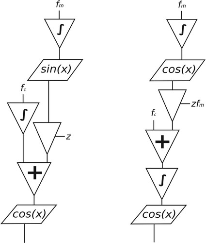
We can see that the FM spectrum of Equation (1(1) $c(t)=\cos (2\pi {\int }_0^t{f}_c+m(x)\mathrm{d}x).$(1) ) (and its corresponding PM expression, Equation (2(2) $c(t)=\cos (\varphi (t)),$(2) )) is composed of partials at $f_c\pm n{f}_m$ Hz, which are scaled by the corresponding Bessel function coefficient $J_n(z)$. We now have a mechanism to represent FM in terms of PM, which provides a clear route for analysis. The two methods have distinct implementations, a comparison between the FM and PM flowcharts is shown in Figure 1.

Figure 1. Flowcharts for PM (left) and FM (right).

4. Second-Order FM

The case of Equation (1(1) $c(t)=\cos (2\pi {\int }_0^t{f}_c+m(x)\mathrm{d}x).$(1) ) is that of first-order modulation, consisting of one modulator and one carrier oscillator. We now consider the arrangement whereby this is increased to a second order, that is, where two modulation stages are present. An FM carrier wave is then used as a modulator to a subsequent carrier oscillator. This can then be extended to higher orders where the output signal is the result of several stages of modulation. It has been claimed in the literature that, unlike PM, FM synthesis cannot be implemented in higher-order topologies (Pinkston, 2000), but as we will demonstrate, that is not the case.

Many of the difficulties arise from a simplistic approach to the implementation of FM synthesis that does not take into account the differences we have discussed in Section 3.1. It is also the case that some synthesisers implement direct forms of FM allowing the possibility of stacked modulation (and even feedback) (see for instance Novation, 2019). However, there are deficiencies in these designs, which we address in this paper. Our motivation here is to develop the hoFM method to produce results that are similar to PM.

4.1. Analysis

We first need to consider the amount of modulation required at each stage. A naïve approach, following directly from the single-level example, would lead us to apply simply the product of an index of modulation $z_n$ and modulation frequency $f_{m_n}$ to determine the frequency deviation at each stage n + 1. If we aim to achieve a spectrum similar to PM, not only is this incorrect from a mathematical point of view, but we may also observe some problematic results.

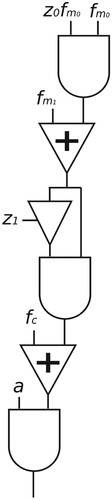
As an example of the pitfalls involved in a simplistic approach, we may consider the case of a particular second-order frequency modulation stack. In this we have a first order modulator with frequency $f_{m_0}$, modulating a second-order modulator with frequency $f_{m_1}$, which then modulates a carrier oscillator with frequency $f_c$, where we set $f_{m_0}=f_{m_1}=f_c$. The FM expression is thus (8) $c(t)=\mathrm{acos}(2\pi {\int }_0^t{f}_c+d_1{m}_1(x)\mathrm{d}x),$(8) and the carrier is modulated by the signal $m_1(t)$ from the first order stage, (9) $m_1(t)=\cos (2\pi {\int }_0^t{f}_{m_1}+d_0{m}_0(x)\mathrm{d}x),$(9) with $m_0(t)=\cos (2\pi f_{m_0}t)$. This naïve FM stack is depicted in Figure 2.

Figure 2. Naïve second-order FM stack.

We know from Equation (7(7) $\cos (\omega +\frac{d}{f_m}\sin (\theta ))=\sum _{n=-\mathrm{\infty }}^{\mathrm{\infty }}{J}_n\left(\frac{d}{f_m}\right)\cos (\omega +\mathrm{n\theta }),$(7) ) that the resulting spectrum of $m_1(t)$ will contain partials at $f_{m_1}\pm n{f}_{m_0}$. For n = −1, we have a component at $f_{m_1}-f_{m_0}=0$ Hz (DC), whose amplitude is given by $-J_1(d_0/f_{m_0})$. When this modulation signal is then applied to the frequency $f_c$ of the carrier oscillator at the next stage, the DC term is simply added as an offset to $f_c$. We can see now that this will result in a shift of the carrier frequency that is proportional to $-d_1{J}_1(d_0/f_{m_0})$. Changes in the modulation index at the top level will then imply a carrier drift. Worse, a change in $d_1$ will also cause $f_c$ to be scaled further.

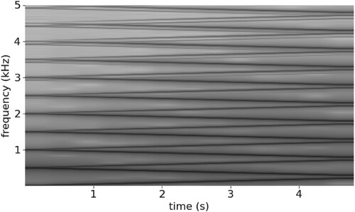
Such an effect ties in timbral changes with partial glides, which in most cases makes it difficult to implement dynamic spectra. Generally with standard FM/PM we should not expect any shift in partial frequencies as we increase or decrease the amount of modulation. There is a separation between the setting of partial frequencies, which is dependent on the ratios of modulators and carrier, and the partial amplitudes, given by the index of modulation. In Figures 3 and  4, we can see the result of applying a change of index of modulation to the $m_0(t)$ and $m_1(t)$ signals, respectively, using a linear envelope from 0 to 2. In these spectrograms, it is possible to see how the change in the amount of modulation at both levels has an effect on the partial frequencies, make them glide divergently as the carrier frequency drifts.

Figure 3. Spectrogram of naïve second-order stacked FM output, with $f_{m_0}=f_{m_1}=f_c=500$ Hz, $d_1=f_{m}0$, applying a linear envelope to $d_0$, $0\le d_0<2f_{m_0}$.

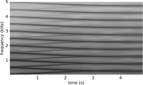
Figure 4. Spectrogram of naïve second-order stacked FM output, with $f_{m_0}=f_{m_1}=f_c=500$ Hz, $d_0=f_{m}0$, applying a linear envelope to $d_1$, $0\le d_1<2f_{m_1}$.

It is of course possible to select modulation frequency ratios that do not result in the modulation signals producing any DC components, and also to produce spectra with a strict $-\pi /2$ (sine) phase at 0 Hz. However these solutions are not general enough to support a theory of higher-order FM synthesis.

Note that such issues do not occur in PM, since any DC offset is translated as a phase shift, rather than a carrier frequency drift. For this reason, as we have already indicated, it is generally much more flexible to adopt PM as a general method for higher-order modulation. We can conclude that a satisfactory solution could be developed by deriving a PM-equivalent form for second-order FM. Using the principles developed earlier, we observe that the integration involved in FM synthesis (cf Equation (1(1) $c(t)=\cos (2\pi {\int }_0^t{f}_c+m(x)\mathrm{d}x).$(1) )) requires that some form of periodic time-varying deviation is applied to the signal. Since the instantaneous frequency of an FM signal is time-varying, it implies the presence of an amplitude modulation term following integration. We now conclude that we need to apply both FM and AM concurrently in the modulation stack.

To demonstrate this, let's review Equations (8(8) $c(t)=\mathrm{acos}(2\pi {\int }_0^t{f}_c+d_1{m}_1(x)\mathrm{d}x),$(8) ) and (9(9) $m_1(t)=\cos (2\pi {\int }_0^t{f}_{m_1}+d_0{m}_0(x)\mathrm{d}x),$(9) ). We are trying to generate a modulation signal $m_1(t)$ whose frequency $f_{m_1}$ is itself modulated by a sinusoidal signal $m_0(t)$, whose frequency is $f_{m_0}$. If we want to apply an index of modulation $z_0$, then according to Equation (6(6) $z=\frac{d}{f_m}.$(6) ), we need to set the $m_0(t)$ signal amplitude $d_0$ to $z_0{f}_{m_0}$. The time-varying frequency $f(t)$ of the modulator $m_1(t)$ is then (10) $f(t)=f_{m_1}+z_0{f}_{m_0}{m}_0(t),$(10) Therefore, also according to Equation (6(6) $z=\frac{d}{f_m}.$(6) ), we need to employ the following time-varying deviation, with an appropriate value of $z_1$, (11) $d_1(t)=z_{1}f(t)=z_1[f_{m_1}+z_0{f}_{m_0}{m}_0(t)],$(11) in order to produce the frequency modulation signal $d_1(t)m_1(t)$, which we will use to modulate the frequency of the carrier oscillator. With this, we have produced a PM-equivalent modulation signal.

4.2. Synthesis

Using the notions developed earlier, we can now describe the PM-equivalent form of second-order FM as (12) $\begin{array}{rl}& m_0(t)=\cos (2\pi f_{m_0}t)\\ & m_1(t)=\cos (2\pi {\int }_0^t{f}_{m_1}+z_0{f}_{m_0}{m}_0(x)\mathrm{d}x)\\ & c(t)=\cos (2\pi {\int }_0^t{f}_c\\ & +z_1[f_{m_1}+z_0{f}_{m_0}{m}_0(x)]m_1(x)\mathrm{d}x\phantom{\int }).\end{array}$(12) From these equations, we can see that the modulator at level 1, $m_1(t)$, is amplitude modulated by its own modulator, $m_0(t)$, when applied to the carrier frequency. We will be able to build on this principle later on, as we extend the method to higher orders. We can now demonstrate how these equations are equivalent to the typical form of second-order PM. To do this, we begin by reworking the first-order modulation as a PM expression, (13) $\begin{array}{rl}& m_0(t)=\sin (2\pi f_{m_0}t)\\ & \varphi (t)=\cos (2\pi f_{m_1}t+z_0{m}_0(t))\\ & c(t)=\cos (2\pi {\int }_0^t{f}_c\\ & +z_1[f_{m_1}+z_0{f}_{m_0}\cos (2\pi f_{m_0}x)]\varphi (x)\mathrm{d}x\phantom{\int }).\end{array}$(13) The next step is to replace $\varphi (\cdot )$ in the carrier signal equation, (14) $\begin{array}{rl}c(t)& =\cos (2\pi {\int }_0^t{f}_c+z_1[f_{m_1}+z_0{f}_{m_0}\cos (2\pi f_{m_0}x)]\\ & \times \cos (2\pi f_{m_1}x+z_0\sin (2\pi f_{m_0}x))\mathrm{d}x\phantom{{\int }_0^t}\phantom{\int }),\end{array}$(14) which translates as the following expression describing second-order PM (15) $c(t)=\cos (2\pi f_{c}t+z_1\sin (2\pi f_{m_1}t+z_0\sin (2\pi f_{m_0}t))).$(15) The equivalent FM topology (Equation (12(12) $\begin{array}{rl}& m_0(t)=\cos (2\pi f_{m_0}t)\\ & m_1(t)=\cos (2\pi {\int }_0^t{f}_{m_1}+z_0{f}_{m_0}{m}_0(x)\mathrm{d}x)\\ & c(t)=\cos (2\pi {\int }_0^t{f}_c\\ & +z_1[f_{m_1}+z_0{f}_{m_0}{m}_0(x)]m_1(x)\mathrm{d}x\phantom{\int }).\end{array}$(12) )) can be implemented using the flowchart shown in Figure 5. In this, we see that in order to implement stacked FM we need to take into account the amplitude modulation effects that arise from employing a modulated input, as per Equation (11(11) $d_1(t)=z_{1}f(t)=z_1[f_{m_1}+z_0{f}_{m_0}{m}_0(t)],$(11) ).

Figure 5. Second-order FM flowchart.

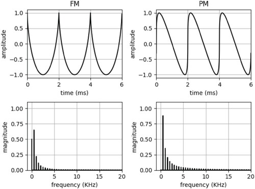
Continuous-time waveforms and their spectra produced by second-order FM and PM are shown to be exactly equivalent in Figure 6. These signals were produced using the approach described by Equation (12(12) $\begin{array}{rl}& m_0(t)=\cos (2\pi f_{m_0}t)\\ & m_1(t)=\cos (2\pi {\int }_0^t{f}_{m_1}+z_0{f}_{m_0}{m}_0(x)\mathrm{d}x)\\ & c(t)=\cos (2\pi {\int }_0^t{f}_c\\ & +z_1[f_{m_1}+z_0{f}_{m_0}{m}_0(x)]m_1(x)\mathrm{d}x\phantom{\int }).\end{array}$(12) ) and Figure 5, in the case of FM, and the corresponding PM expression given in Equation (15(15) $c(t)=\cos (2\pi f_{c}t+z_1\sin (2\pi f_{m_1}t+z_0\sin (2\pi f_{m_0}t))).$(15) ). We have now demonstrated that it is indeed possible to use a second-order FM topology to produce a spectrum that is similar to second-order PM. This solves the issues identified earlier as illustrated by Figures 3 and 4, as we know that stacked PM does not suffer from them.

Figure 6. Second-order FM (left) and PM (right) waveforms and normalised spectra from Equation (12(12) $\begin{array}{rl}& m_0(t)=\cos (2\pi f_{m_0}t)\\ & m_1(t)=\cos (2\pi {\int }_0^t{f}_{m_1}+z_0{f}_{m_0}{m}_0(x)\mathrm{d}x)\\ & c(t)=\cos (2\pi {\int }_0^t{f}_c\\ & +z_1[f_{m_1}+z_0{f}_{m_0}{m}_0(x)]m_1(x)\mathrm{d}x\phantom{\int }).\end{array}$(12) ) (Figure 5) and Equation (15(15) $c(t)=\cos (2\pi f_{c}t+z_1\sin (2\pi f_{m_1}t+z_0\sin (2\pi f_{m_0}t))).$(15) ), respectively, with $f_c=f_{m_0}=f_{m_1}=500$ Hz, $z_0=3$, and $z_1=2$.

4.3. Spectrum

With its equivalent PM form, we can now derive an expression for the second-order FM spectrum. Using Equation (4(4) $\begin{array}{rl}{e}^{\pm \mathrm{jzsin}(\theta )}& =J_0(z)+2\sum _{n=1}^{\mathrm{\infty }}{J}_{2n}(z)\cos \left(2\mathrm{n\theta }\right)\\ & \pm 2j\sum _{n=0}^{\mathrm{\infty }}{J}_{2n+1}(z)\sin ([2n+1]\theta ),\end{array}$(4) ) we rewrite Equation (15(15) $c(t)=\cos (2\pi f_{c}t+z_1\sin (2\pi f_{m_1}t+z_0\sin (2\pi f_{m_0}t))).$(15) ) as (16) $\begin{array}{rl}c(t)& =\cos (\phantom{\sum _{n=-\mathrm{\infty }}^{\mathrm{\infty }}}2\pi f_{c}t\\ & +z_1\sum _{n=-\mathrm{\infty }}^{\mathrm{\infty }}{J}_n(z_0)\sin (2\pi [f_{m_1}+n{f}_{m_0}]t)).\end{array}$(16) From this equation we can now use a derivation of the spectrum of complex PM (LeBrun, 1977). In order to make this more meaningful, we assume that the first-order output signal spectrum contains only $K_0$ sidebands with significant energy (rather than the theoretically non-bandlimited spectrum). The expansion of the second-order FM synthesis equation can then be given as (17) $\begin{array}{rl}& \sum _{{\eta }_{-K_0}=-\mathrm{\infty }}^{\mathrm{\infty }}\dots \sum _{{\eta }_{K_0}=-\mathrm{\infty }}^{\mathrm{\infty }}\prod _{k_0=-K_0}^{K_0}{J}_{{\eta }_{k_0}}(z_1{J}_{k_0}(z_0))\\ & \cos (2\pi [f_c+\sum _{k_0=-K_0}^{K_0}{\eta }_{k_0}(f_{m_1}+k_0{f}_{m_0})]t).\end{array}$(17) The value of $K_0$ is dependent on the first-order modulation index $z_0$ and will increase as more modulation is inserted into the signal. We should note that Equation (17(17) $\begin{array}{rl}& \sum _{{\eta }_{-K_0}=-\mathrm{\infty }}^{\mathrm{\infty }}\dots \sum _{{\eta }_{K_0}=-\mathrm{\infty }}^{\mathrm{\infty }}\prod _{k_0=-K_0}^{K_0}{J}_{{\eta }_{k_0}}(z_1{J}_{k_0}(z_0))\\ & \cos (2\pi [f_c+\sum _{k_0=-K_0}^{K_0}{\eta }_{k_0}(f_{m_1}+k_0{f}_{m_0})]t).\end{array}$(17) ) is reduced to Equation (7(7) $\cos (\omega +\frac{d}{f_m}\sin (\theta ))=\sum _{n=-\mathrm{\infty }}^{\mathrm{\infty }}{J}_n\left(\frac{d}{f_m}\right)\cos (\omega +\mathrm{n\theta }),$(7) ) if $z_0=0$, (18) $\sum _{{\eta }_0=-\mathrm{\infty }}^{\mathrm{\infty }}{J}_{{\eta }_0}\left(z_1\right)\cos (2\pi [f_c+{\eta }_0{f}_{m_1}]t),$(18) since in this case there is no modulation at the first-order stage, $K_0=0$, and $J_0(0)=1$. From Lazzarini (2021), a reasonable estimate for this can be found as $K_0\approx z_0+l$, $z_0>1$, with $2⪅l⪅3$. Using a similar approximation for the number of second-order sidebands based on $z_1$, the case of Figure 6 is thus given by (19) $\begin{array}{rl}& \sum _{{\eta }_{-5}=-4}^4\dots \sum _{{\eta }_5=-4}^4\prod _{k_0=-5}^5{J}_{{\eta }_{k_0}}(2J_{k_0}(3))\\ & \cos (2\pi [f_0+\sum _{k_0=-5}^5{\eta }_{k_0}{f}_0(k_0+1)]t),\end{array}$(19) with $f_0=500$ Hz. We can observe in Figure 6 that this second-order FM/PM spectrum extends to a 15,500 Hz partial at −90 dB, and the above expression with K = 5 describes the spectrum up to 12,500 Hz (∼70 dB below the loudest harmonic).

This derivation of the second-order FM spectrum brings to the fore two important aspects. Firstly, we should note that, as indicated by Equation (17(17) $\begin{array}{rl}& \sum _{{\eta }_{-K_0}=-\mathrm{\infty }}^{\mathrm{\infty }}\dots \sum _{{\eta }_{K_0}=-\mathrm{\infty }}^{\mathrm{\infty }}\prod _{k_0=-K_0}^{K_0}{J}_{{\eta }_{k_0}}(z_1{J}_{k_0}(z_0))\\ & \cos (2\pi [f_c+\sum _{k_0=-K_0}^{K_0}{\eta }_{k_0}(f_{m_1}+k_0{f}_{m_0})]t).\end{array}$(17) ), the resulting spectrum may be very complex and difficult to predict if $z_0$ and $z_1$ are large. In that case there will be many sidebands with frequencies $f_c\pm n_{k_0}{f}_{m_1}\pm k_0{\eta }_{k_0}{f}_{m_0}$ with significant intensity interacting with each other. Secondly, we may reduce second-order FM as a first-order case employing a complex modulator, but with the advantage that we can change the spectrum of the modulating wave via a single parameter, $z_0$. Such an arrangement generally calls for small modulation indices. This is in fact a good reason for employing second (or higher)-order modulation topologies; we find that smoother FM spectral changes are better achieved with indices that range from 0 to a small positive value (Lazzarini, 2021). As in the case of a complex modulating wave, it is possible to achieve partial-rich spectra with much more reduced modulation compared to simple first-order sinusoidal modulation.

5. Higher-order modulation

The method developed here for second-order modulation can be seen as a particular case of hoFM. After proving the equivalence of Equation (12(12) $\begin{array}{rl}& m_0(t)=\cos (2\pi f_{m_0}t)\\ & m_1(t)=\cos (2\pi {\int }_0^t{f}_{m_1}+z_0{f}_{m_0}{m}_0(x)\mathrm{d}x)\\ & c(t)=\cos (2\pi {\int }_0^t{f}_c\\ & +z_1[f_{m_1}+z_0{f}_{m_0}{m}_0(x)]m_1(x)\mathrm{d}x\phantom{\int }).\end{array}$(12) ) to the PM expression given by Equation (15(15) $c(t)=\cos (2\pi f_{c}t+z_1\sin (2\pi f_{m_1}t+z_0\sin (2\pi f_{m_0}t))).$(15) ), we can now extend it to an arbitrarily high order. A stack of modulators of order n is thus given as (20) $\begin{array}{rl}{m}_0(t)& =\cos (2\pi f_{m_0}t)\\ m_1(t)& =\cos (2\pi {\int }_0^t{f}_{m_1}+z_0{f}_{m_0}{m}_0(x)\mathrm{d}x)\\ m_2(t)& =\cos (2\pi {\int }_0^t{f}_{m_2}+z_1[f_{m_1}\\ & +z_0{f}_{m_0}{m}_0(x)]m_1(x)\mathrm{d}x)\\ & \dots \\ m_{n-1}(t)& =\cos (2\pi {\int }_0^t{f}_{m_{n-1}}+z_{n-2}[f_{m_{n-2}}\\ & +z_{n-3}{f}_{m_{n-3}}{m}_{n-3}(x)]m_{n-2}(x)\mathrm{d}x)\\ c(t)& =\cos (2\pi {\int }_0^{t}c+z_{n-1}[f_{m_{n-1}}\\ & +z_{n-2}{f}_{m_{n-2}}{m}_{n-2}(x)]m_{n-1}(x)\mathrm{d}x\phantom{\int }).\end{array}$(20) The modulation signal at each level m, m>0, is amplitude modulated by its own FM input. We observe that in general if a signal whose instantaneous frequency changes significantly over time is used for FM, then we will need to account for this in the integration. From another perspective, we can also observe that through amplitude modulation, we are able to suppress the DC signals responsible for any carrier drift.

The spectrum of stacked FM at order n is duly obtained by extending Equation (17(17) $\begin{array}{rl}& \sum _{{\eta }_{-K_0}=-\mathrm{\infty }}^{\mathrm{\infty }}\dots \sum _{{\eta }_{K_0}=-\mathrm{\infty }}^{\mathrm{\infty }}\prod _{k_0=-K_0}^{K_0}{J}_{{\eta }_{k_0}}(z_1{J}_{k_0}(z_0))\\ & \cos (2\pi [f_c+\sum _{k_0=-K_0}^{K_0}{\eta }_{k_0}(f_{m_1}+k_0{f}_{m_0})]t).\end{array}$(17) ) as (21) $\begin{array}{rl}& [\sum _{{\eta }_{-K_0}=-\mathrm{\infty }}^{\mathrm{\infty }}\dots \sum _{{\eta }_{K_0}=-\mathrm{\infty }}^{\mathrm{\infty }}]\dots [\sum _{{\eta }_{-K_{n-2}}=-\mathrm{\infty }}^{\mathrm{\infty }}\dots \sum _{{\eta }_{K_{n-2}}=-\mathrm{\infty }}^{\mathrm{\infty }}]\\ & \left[\prod _{k_0=-K_0}^{K_0}{J}_{{\eta }_{k_0}}(z_1{J}_{k_0}(z_0))\right]\dots \\ & \left[\prod _{k_{n-2}=-K_{n-2}}^{K_{n-2}}{J}_{{\eta }_{k_{n-2}}}(z_{n-1}{J}_{k_{n-2}}(z_{n-2}))\right]\\ & \cos (2\pi [f_c+\sum _{k_0=-K_0}^{K_0}{\eta }_{k_0}(f_{m_1}+k_0{f}_{m_0})+\cdots \\ & +\sum _{k_{n-2}=-K_{n-2}}^{K_{n-2}}{\eta }_{k_{n-2}}(f_{m_{n-1}}+k_{n-2}{f}_{m_{n-2}})]t),\end{array}$(21) with same approximations $K_m\approx z_m+l$ at each modulation level m. As can be seen, the complexity of the spectrum can increase significantly depending on the order, the modulation frequencies and indices.

5.1. Operators

In order to facilitate the design of instruments using hoFM, we can take advantage of the concept of an operator. At its simplest, this is a sinusoidal oscillator whose frequency can be modulated by another. The principle of an operator is very common in PM synthesis (Chowning & Bristow, 1986), and it may also include an envelope to allow for dynamic spectra as well as amplitude shaping. In PM, an operator is characterised by a phase modulation input, plus amplitude and frequency parameters, and a single output. Operators can be connected in series (stacked), or in parallel. For FM, we can develop a similar black-box approach.

To design an operator for FM, we need to take account of our analysis in Section 4. We may note that within a stack, the top oscillator takes in a modulation frequency and a modulation index, producing a modulation signal. Subsequent oscillators take in a modulation signal in addition to the frequency and index. At the bottom of the stack, an oscillator produces the output signal, and it takes an amplitude instead of a modulation index. As in PM, the operator takes three inputs (index/amplitude and frequency scalars plus modulation signal). The specification requires that we make no distinction between amplitude and index. For this to be practical, unlike in the PM case, we would then need to distinguish between audio and modulation outputs. For this reason, a freely-stackable FM operator requires two separate outputs. Envelopes may be added to shape the scalar input parameters. In pseudocode, the simplest design would be

With this, the second-order stack discussed earlier would be defined as

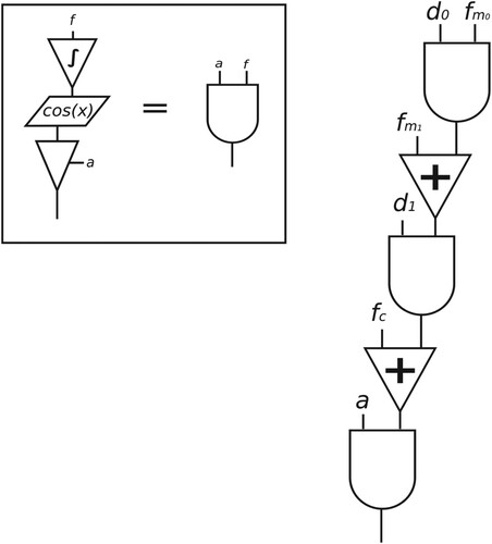
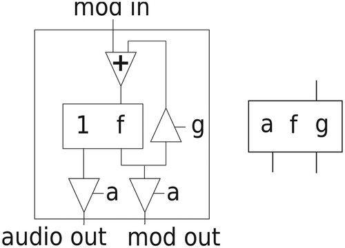
The implementation of the operator black box is shown in Figure 7, together with an arrangement of three operators in a second-order modulation topology equivalent to that of Figure 5.

Figure 7. FM operator (left) and second-order modulation arrangement (right). The a and f parameters represent the scalar index/amplitude and frequency.

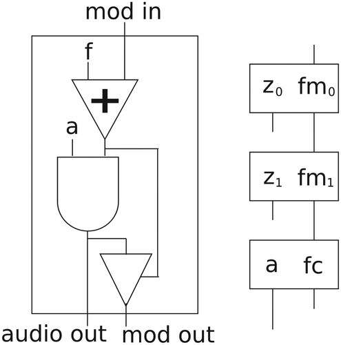
As can be seen, the actual signal flow is re-ordered somewhat with the product being placed at the output of the oscillator. This way it is possible to use a single operator as either a carrier or a modulator in any arrangement of any order. The topmost modulator will always have no signal inputs and we only use the audio signal out of the carrier operator. Also we should note that this allows us to tap anywhere into a hoFM topology to retrieve an audio signal at that point. Dynamic spectra can be implemented by including envelopes to control the a and f parameters in Figure 5.

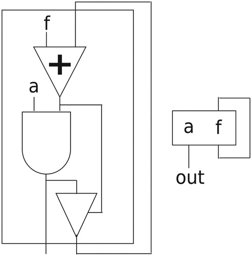
5.2. Feedback

The operator as developed here opens up the possibility of implementing a feedback FM design, which is analogous to feedback PM as introduced by Tomisawa (1979). Confusingly, his technique has been called feedback FM in the literature, which only served to muddy the waters. We should continue to make the distinctions we made before between FM and PM, thus we will refer to Tomisawa's method as feedback PM, and our method as feedback hoFM.

Feedback hoFM can be thought of as a form of hoFM where an infinite number of modulators are stacked, all with the same frequency. To construct this, we just need to apply the modulation recursively, as in

which is depicted as a flowchart in Figure 8.

Figure 8. FM operator with feedback (left) and its black-box representation (right).

For an operator with unity amplitude whose frequency is $f_0$, the feedback hoFM formula arising from its arrangement can then be put as (22) $\omega (t)=\cos (2\pi {\int }_0^t[f_0+\omega (x)]\omega (x)\mathrm{d}x),$(22) which seems intractable at first. However, after Mitsuhashi (1982), we can determine a complex PM expression that is equivalent to it, (23) $\omega (t)=\cos (2\pi f_{0}t+2\sum _{n=1}^{\mathrm{\infty }}\frac{J_n(n)}{n}\sin (2\mathrm{\pi n}{f}_{0}t))$(23) This corresponds to a cosine whose phase is modulated by a complex waveform $m(t)$. A similar expression can also be used to describe the elliptic motion of a planet about the sun, as shown by Lagrange in 1770 (Watson, 1944, p. 6). From there we can derive the spectrum of feedback hoFM as (24) $\omega (t)=-\frac{1}{2}+2\sum _{n=1}^{\mathrm{\infty }}\frac{{\dot{J}}_n(n)}{n}\cos (2\mathrm{\pi n}{f}_{0}t),$(24) with $2{\dot{J}}_n(n)=J_{n-1}(n)-J_{n+1}(n)$. It is interesting to note that in this case, the spectral description is considerably more simplified and compact than in the general case of hoFM as shown by Equation (21(21) $\begin{array}{rl}& [\sum _{{\eta }_{-K_0}=-\mathrm{\infty }}^{\mathrm{\infty }}\dots \sum _{{\eta }_{K_0}=-\mathrm{\infty }}^{\mathrm{\infty }}]\dots [\sum _{{\eta }_{-K_{n-2}}=-\mathrm{\infty }}^{\mathrm{\infty }}\dots \sum _{{\eta }_{K_{n-2}}=-\mathrm{\infty }}^{\mathrm{\infty }}]\\ & \left[\prod _{k_0=-K_0}^{K_0}{J}_{{\eta }_{k_0}}(z_1{J}_{k_0}(z_0))\right]\dots \\ & \left[\prod _{k_{n-2}=-K_{n-2}}^{K_{n-2}}{J}_{{\eta }_{k_{n-2}}}(z_{n-1}{J}_{k_{n-2}}(z_{n-2}))\right]\\ & \cos (2\pi [f_c+\sum _{k_0=-K_0}^{K_0}{\eta }_{k_0}(f_{m_1}+k_0{f}_{m_0})+\cdots \\ & +\sum _{k_{n-2}=-K_{n-2}}^{K_{n-2}}{\eta }_{k_{n-2}}(f_{m_{n-1}}+k_{n-2}{f}_{m_{n-2}})]t),\end{array}$(21) ).

It is also noteworthy to contrast this with feedback PM (Tomisawa, 1979), defined by (25) $\varphi (t)=\sin (2\pi f_{0}t+\varphi (t)),$(25) which actually corresponds to $m(t)$ (Benson, 2008, p. 62), (26) $\varphi (t)=2\sum _{n=1}^{\mathrm{\infty }}\frac{J_n(n)}{n}\sin (2\mathrm{\pi n}{f}_{0}t).$(26) Since $2\frac{J_n(n)}{n}\approx \frac{1}{n}$, this is very nearly a sawtooth wave.

The spectrum and waveform of feedback hoFM is shown on Figure 9 alongside feedback PM. As we can see, if we exclude the negative DC term, the two spectra share many similarities, although the waveforms are different. This is mostly to do with different partial phases. While the feedback PM formula produces an odd waveform, therefore a purely imaginary spectrum, feedback hoFM results in an even waveform, featuring a purely real spectrum. This is due to the fact that sine wave modulators are guaranteed to produce only sine wave sidebands with a sine carrier and a strictly cosine wave spectrum with a cosine carrier (cf Lazzarini, 2021, chap. 8). We also observe that the feedback hoFM spectral envelope has slightly more accentuated rolloff, defined by a ${\dot{J}}_n(n)/J_n(n)$ factor for each harmonic n.

Figure 9. Feedback hoFM (left) and PM (right) waveforms and spectra, with f = 500 Hz.

Dynamic spectra in this arrangement become possible through applying an envelope to the amplitude a, $|a|\le 1$, of the operator, resulting in (27) $-\frac{a^2}{2}+2a\sum _{n=1}^{\mathrm{\infty }}\frac{{\dot{J}}_n(\mathrm{an})}{n}\cos (2\mathrm{\pi n}{f}_{0}t).$(27) As can be seen, a has an effect on both amplitude and bandwidth, as the feedback modulation increases at the same time as the operator output. If we want to decouple these, it is possible to keep the operator amplitude at unity, and employ a separate gain $|g|\le 1$ to control the feedback amount. The amplitude control can then be applied to the audio and modulator outputs. An operator including internal feedback with independent amplitude and bandwidth control is shown in Figure 10.

Figure 10. FM operator including an internal feedback path with independent control of amplitude (a) and feedback gain ($|g|\le 1$) (left) and its black-box representation (right).

Finally, it is important to note the aforementioned technique of loopback FM introduced by Smyth and Hsu (2019), which as opposed to feedback hoFM, does not intend to provide a feedback PM-analogous spectrum. Instead, it employs the output of the oscillator directly to modulate its own frequency, with distinct spectral results. This has received a thorough treatment by Hsu (2019), where it is contrasted to the standard technique of feedback PM.

6. Digital implementation

Following the exposition of the theory in continuous time, we can now turn to look at the implementation of higher-order FM using digital oscillators. We first provide a reference implementation in C++ for an operator, together with a second-order example. This is followed by an analysis of issues arising in digital FM synthesis and practical mitigation methods.

6.1. Reference implementation in C++

The following code provides a reference implementation of the hoFM synthesis operator, including an internal feedback path, as depicted in Figures 7 and 10:

The table lookup oscillator in this implementation employs fixed-point phase computation, thus wavetables are required to have a power-of-two plus one size (the extra point is used for linear interpolation). By employing a fixed-point function table and normalisation factor, the code could also be deployed in platforms with no floating-point support.

Using instances of this class, we can implement various types of hoFM synthesis topologies. For example, a second-order hoFM arrangement, such as the one described in Figure 5, can be modelled using the following code:

An object of this class can then be used to produce a hoFM tone as shown by an example program fragment. It uses modulation frequencies set to $c=m_0=m_1$ with separate indices of modulation for first and second-order stages (z0, z1):

6.2. Issues

We normally expect a digital implementation to produce a signal that is fairly faithful to the continuous-time equations, if enough mathematical precision is employed. However, in practice we observe a certain amount of phase drift whenever an FM signal is generated using digital oscillators, due to errors associated with the use of a discrete-time integrator. As demonstrated by the reference code, the instantaneous phase of a digital oscillator is usually computed using an infinite impulse response filter defined by (28) $y(n)=x(n)+y(n-1),$(28) to which a frequency signal, $x(n)=f(n)/f_s$, is applied (with $f_s$ denoting the sampling frequency). Defining the digital integration filter (Equation (28(28) $y(n)=x(n)+y(n-1),$(28) )) as the operator integ$[.]$, the output of digital FM can be described by (29) $\nu (n)=\cos \left(2\pi \mathrm{integ}\left[\frac{f_{m_1}+z_0{f}_{m_0}\cos \left(2\pi f_{m_0}\frac{n}{f_s}\right)}{f_s}\right]\right).$(29) The net effect of the integration error is to add an extra term to $\varphi (t)$ in Equation (13(13) $\begin{array}{rl}& m_0(t)=\sin (2\pi f_{m_0}t)\\ & \varphi (t)=\cos (2\pi f_{m_1}t+z_0{m}_0(t))\\ & c(t)=\cos (2\pi {\int }_0^t{f}_c\\ & +z_1[f_{m_1}+z_0{f}_{m_0}\cos (2\pi f_{m_0}x)]\varphi (x)\mathrm{d}x\phantom{\int }).\end{array}$(13) ). If we set $t=n/f_s$, we can re-write the phase-modulated modulator $\varphi (t)$ in Equation (13(13) $\begin{array}{rl}& m_0(t)=\sin (2\pi f_{m_0}t)\\ & \varphi (t)=\cos (2\pi f_{m_1}t+z_0{m}_0(t))\\ & c(t)=\cos (2\pi {\int }_0^t{f}_c\\ & +z_1[f_{m_1}+z_0{f}_{m_0}\cos (2\pi f_{m_0}x)]\varphi (x)\mathrm{d}x\phantom{\int }).\end{array}$(13) ) to include this extra term. We now have this equation in a form which is equivalent to the output of a frequency-modulated digital oscillator, (30) $\hat{\varphi }(t)=\cos (2\pi f_{m_1}t+z[\sin (2\pi f_{m_0}t)])+ϵ(t).$(30) The integration error $ϵ(t)$ can be computed as the amplitude difference of the frequency-modulated waveform, $\nu (t)$, and the ideal phase modulation signal, $\varphi (t)$ (Equation (13(13) $\begin{array}{rl}& m_0(t)=\sin (2\pi f_{m_0}t)\\ & \varphi (t)=\cos (2\pi f_{m_1}t+z_0{m}_0(t))\\ & c(t)=\cos (2\pi {\int }_0^t{f}_c\\ & +z_1[f_{m_1}+z_0{f}_{m_0}\cos (2\pi f_{m_0}x)]\varphi (x)\mathrm{d}x\phantom{\int }).\end{array}$(13) ), with $t=n/f_s$), (31) $ϵ(t)=\nu (t)-\varphi (t).$(31) Since the two signals, $\nu (t)$ and $\varphi (t)$ have the same period and are generally similar in shape, we conclude that $ϵ(t)$ is a periodic signal with the same period as the waveform $m_1(t)$, 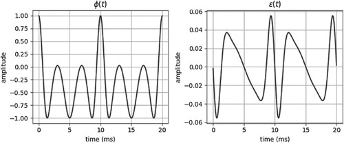and a relatively low amplitude. This is demonstrated by Figure 11, where $\varphi (t)$ and $ϵ(t)$ are shown side-by-side.

Figure 11. Modulation $\varphi (t)$ (left) and error $ϵ(t)$ (right) from Equation (31(31) $ϵ(t)=\nu (t)-\varphi (t).$(31) ), with $f_{m_0}=f_{m_1}=100$ Hz, $z_0=3$, and $f_s=44.1$ KHz.

6.2.1. Second-order error analysis

From Equations (31(31) $ϵ(t)=\nu (t)-\varphi (t).$(31) ) and (12(12) $\begin{array}{rl}& m_0(t)=\cos (2\pi f_{m_0}t)\\ & m_1(t)=\cos (2\pi {\int }_0^t{f}_{m_1}+z_0{f}_{m_0}{m}_0(x)\mathrm{d}x)\\ & c(t)=\cos (2\pi {\int }_0^t{f}_c\\ & +z_1[f_{m_1}+z_0{f}_{m_0}{m}_0(x)]m_1(x)\mathrm{d}x\phantom{\int }).\end{array}$(12) ), the equation for second-order FM, as produced by a digital oscillator, becomes (32) $\begin{array}{rl}c(t)& =\cos (2\pi {\int }_0^t{f}_c+z_1[f_{m_1}+z_0{f}_{m_0}\cos (2\pi f_{m_0}x)]\\ & \times [\cos (2\pi f_{m_1}x-z_0[\sin (2\pi f_{m_0}x)])+ϵ(x)]\mathrm{d}x\phantom{\int })\end{array}$(32) Translating this into a PM expression, we have (33) $\begin{array}{rl}c(t)& =\cos (2\pi f_{c}t+z_1\sin (2\pi f_{m_1}t\\ & +z_0\sin (2\pi f_{m_0}t))+\theta (t)),\end{array}$(33) which excludes a low-amplitude term due to the carrier phase drift. Similarly to what we have observed in $\hat{\varphi }(t)$, it does not contribute too much to the overall signal spectrum. The $\theta (t)$ function is therefore the significant differing factor between the ideal PM representation of second-order FM and its realisation with digital oscillators. It can be characterised as a slow phase modulation term that is dependent on the phase drift of the frequency-modulated oscillator, (34) $\dot{\theta }(t)=z_1[f_{m_1}+z_0{f}_{m_0}\cos (2\pi f_{m_0}t)]ϵ(t).$(34) The nature of $ϵ(t)$, and by consequence $\theta (t)$, is important. If the former contains any DC term, the integration turns this into a linear modulation function, resulting in a low-frequency phase modulation of the carrier wave. If there is no DC, then the errors are only responsible for a small fixed difference in the shape of the FM signal in comparison to the corresponding PM formulation.

Following these general ideas, we can proceed with a further analysis of the integration error signal. The amplitude of $ϵ(t)$ is inversely proportional to the sampling frequency; it is also proportional to the modulation frequency. The error signal $ϵ(t)$ can be described as a phase-modulated carrier wave, and so we can predict that its components exist at $f_{m_1}\pm n{f}_{m_0}$ Hz. Therefore, if $f_{m_0}=f_{m_1}$, we should expect a DC term with a certain amount of prominence in this signal, leading to low-frequency phase modulation artefacts, unless the phase of the DC component can be made to be exactly $|\pi /2|$ (that is, an absolute sine phase). On the other hand, by setting $f_{m_0}=2f_{m_1}$, we are able to suppress the slow phase modulation term (as no DC component is present in the FM signal), producing a steady output.

6.2.2. Mitigation

In the case of hoFM, the most adverse effects of digital integration errors have to do with the appearance of a low-frequency phase modulation term in the carrier wave. Furthermore, we may also observe these in feedback hoFM, where they can cause a small but perceived pitch detuning that is dependent on the feedback amount. These effects may be mitigated in four ways:

1. Limit the $f_{m_n}:\cdots :f_{m_1}:f_{m_0}$ ratios to values where no sideband is present at 0 Hz.

2. Judiciously choose a phase offset for $m_0(t)$ (etc) so that the spectrum of $\theta (t)$ does not contain any energy, by forcing any 0 Hz sideband to be produced with a $|\pi /2|$ phase offset. This modulator offset is a function of the modulation index $z_0$ (etc) and is independent of the modulation frequency;

3. computing a phase error signal that can be subtracted from $\nu (t)$.

4. Employ an oversampling factor such as to minimise any integration errors.

Of these, the first measure does not provide a general solution to the problem, it cannot be applied to feedback, and we are back more or less where we started. The second solution is more promising, such offsets can be computed for different configurations and stored in lookup tables. This may be a practical solution in cases where computing cost is at a premium. The third method somehow defeats the purpose of the overall approach: if we have a good means of generating a phase modulation signal, then employing FM does not seem to be ideal. However, the latter can be a good method for error analysis, as demonstrated earlier in this section, rather than one used in deployment.

The final solution is probably the most practical: if we can approximate the continuous-time expression with a very fine degree of accuracy, we will not only be suppressing the integration errors, but we will also avoid any issues with foldover that may arise in the carrier wave spectrum (depending on the indices of modulation employed). It is often the case that FM/PM is prone to aliasing distortion. By oversampling, as is commonly done for instance with virtual analogue filters and oscillators (Pakarinen et al., 2011), we can solve these two issues at the same time.

As an example, we can efficiently incorporate oversampling in the hoFM code example shown earlier using secret rabbit code (de Castro Lopo, 2023),

In this C++ class, we may set the oversampling factor ovs to achieve the mitigation effect described above depending on the original sampling rate used. In our tests, we have experimentally observed that an oversampling factor of 4 is sufficient to reduce artefacts significantly. Since these are related both to the sampling rate and the modulation frequencies applied, higher modulation frequencies may require us to increase this oversampling factor. In systems where the sampling rate is normally high, e.g. in the case of field programmable gate array (FPGA) oscillators, no oversampling is required and the methods described here find an optimal implementation platform.

7. Conclusions

A simplistic approach to implementing second and higher-order FM arrangements has been shown to have limitations. Typical issues found in these situations are related to carrier drift, which is due to the presence of a DC component in a modulating waveform. Since the amount of energy at 0 Hz is defined by the index of modulation and is a function of the Bessel coefficient associated with the relevant sideband, any timbral changes in this case are accompanied by frequency glides that may be objectionable in practical applications. Such issues, caused by DC offsets in modulators, which also may pose practical limits to the use of feedback, are fully solved through the development of the PM-equivalent method of hoFM. Since higher-order PM is well understood and has been successfully applied in a variety of contexts, we propose that this may be a more suitable approach.

In this paper, we defined in detail the differences between PM and FM, stemming from the fact that integration is directly present in the modulation of frequency. For this reason, to achieve a degree of control of higher-order modulation, care needs to be taken to ensure that these differences are duly respected. This means that it is not possible to solely employ the modulation signal to modify the frequency of the oscillator, but we also need to modulate its amplitude. From these results, we then proposed a second-order FM arrangement that represents a PM-equivalent synthesis equation. From this formula we are then able to describe the resulting FM spectrum by employing a similar approach to the derivation of the complex PM spectrum.

The technique of hoFM can then be implemented as an extension of this second-order arrangement. For this, we found that an operator approach may be helpful. We have then put forward the basic design of such a black box, demonstrating its equivalence to the second-order design shown earlier. With these, it is possible to freely construct various hoFM topologies, including feedback hoFM, as it is customarily done with PM. We completed the discussion with a full reference implementation of operator-based hoFM.

While it was beyond the scope of this paper to consider in detail possible applications of hoFM synthesis, we may cite a few. Generally, the technique is useful in situations where it is not convenient or practical to modulate the phase of a signal. One such example is the case of the synthesis methods employed in the Summit synthesiser oscillator implementation (Novation, 2019). Although these have not been published and it is not possible to exactly determine their details, it is a reasonable assumption that PM is either not possible or not ideal since they opted to implement stacked FM in a somewhat simpler form (as per our earlier analysis). Another application may be found in analogue signal processing, where it is often the case that (linear) FM can be employed directly, whereas PM poses more difficulties (Lazzarini & Timoney, 2021). Thus a simplification in circuit design may be also another factor that would favour the use of the technique.

Within a digital signal processing environment, however, we have noted that there are a few practical issues arising within the scenarios of stacked and feedback hoFM introduced here. These have to do with numerical errors arising from the discrete nature of the integration filter employed in the implementation of an oscillator. In the case of a modulation stack, we have observed that such errors result in a phase modulation term that is not present in the continuous-time analysis of Section 4. This can introduce periodic modulation artefacts in the carrier signal that may be objectionable. In the case of feedback hoFM, the errors insert an extraneous DC term in the signal that has an obvious, although small, effect on pitch. We provided an analysis of these errors, their effects, and possible mitigation. In some applications, such as the extremely high sampling rate oscillator implementations (e.g. using FPGA hardware, as in the case of Summit synthesiser, running in the two-digit MHz range), these digital signal processing issues may not be of concern. Developers in specialist digital platforms, and practitioners of analogue synthesis may find benefit from the theory and practice of hoFM.

Code examples and scripts used for the signal analysis in this paper can be found at https://github.com/vlazzarini/highorderfm

Disclosure statement

No potential conflict of interest was reported by the author(s).

References

- Benson, D. (2008). Music, a mathematical offering. Oxford University Press.
- Bloch, A. (1944). Modulation theory. Journal of the Institution of Electrical Engineers -- Part I: General, 91(45), 368–370.
- Carson, J. (1922). Notes on the theory of modulation. Proceedings Institute of Radio Engineers, 10(1), 57–64.
- Caspe, F., McPherson, A., & Sandler, M. (2022). DDX7: Differentiable FM synthesis of musical instrument sounds. In Proceedings of the 23rd ISMIR conference (pp. 608–615). ISMIR.
- Chowning, J. (1973). The synthesis of complex audio spectra by means of frequency modulation. Journal of the Audio Engineering Society, 21(7), 527–534.
- Chowning, J., & Bristow, D. (1986). FM theory and applications. Yamaha Music Foundation.
- Corrington, M. S. (1947). Variation of bandwidth with modulation index in frequency modulation. Proceedings of the IRE, 35(10), 1013–1020. https://doi.org/10.1109/JRPROC.1947.231588
- de Castro Lopo, E. (2023). Secret rabbit code. Retrieved May 17, 2023, from https://libsndfile.github.io/libsamplerate/index.html.
- Gabor, D. (1940). Theory of communication. Journal of the Institution of Electrical Engineers -- Part III: Radio and Communication Engineering, 93(26), 429–457.
- Horner, A. (1996). Double-modulator FM matching of instrument tones. Computer Music Journal, 20(2), 57–71. Retrieved May 24, 2023, from http://www.jstor.org/stable/3681332.
- Horner, A. (1998, August). Nested modulator and feedback FM matching of instrument tones. Speech and Audio Processing, IEEE Transactions on, 6, 398–409. https://doi.org/10.1109/89.701371
- Horner, A., Beauchamp, J., & Haken, L. (1993). Machine tongues XVI: Genetic algorithms and their application to FM matching synthesis. Computer Music Journal, 17(4), 17–29. Retrieved May 24, 2023, from, http://www.jstor.org/stable/3680541
- Hsu, J. (2019). Physically-informed percussion synthesis with nonlinearities for real-time applications [Unpublished doctoral dissertation]. University of California San Diego.
- Hutchins, B. (1975). The frequency modulation spectrum of an exponential voltage-controlled oscillator. Journal of the Audio Engineering Society, 23(3), 200–207.
- Lazzarini, V. (2017). Computer music instruments. Springer.
- Lazzarini, V. (2021). Spectral music design: A computational approach. Oxford Univ. Press.
- Lazzarini, V., Keller, D., & Radivojević, N. (2023). Issues of ubiquitous music archaeology: Shared knowledge, simulation, terseness, and ambiguity in early computer music. Frontiers in Signal Processing, 3, 1132672. https://doi.org/10.3389/frsip.2023.1132672
- Lazzarini, V., & Timoney, J. (2010). Theory and practice of modified frequency modulation synthesis. Journal of the Audio Engineering Society, 58(6), 459–471.
- Lazzarini, V., & Timoney, J. (2021). Modulation synthesis in digital and analogue computing environments. In Proceedings of the 11th ubiquitous music workshop (pp. 104–116). Ubiquitous Music Group.
- Lazzarini, V., Timoney, J., & Lysaght, T. (2008). The generation of natural-synthetic spectra by means of adaptive frequency modulation. Computer Music Journal, 32(2), 9–22. https://doi.org/10.1162/comj.2008.32.2.9
- LeBrun, M. (1977). A derivation of the spectrum of FM with a complex modulating wave. Computer Music Journal, 1(4), 51–52.
- LeBrun, M. (1979). Digital waveshaping synthesis. Journal of the Audio Engineering Society, 27(4), 250–266.
- Mitsuhashi, Y. (1982). Musical sound synthesis by forward differences. Journal of the Audio Engineering Society, 30(1/2), 1–9.
- Moore, F. R. (1990). Elements of computer music. Prentice-Hall, Inc.
- Moorer, J. (1977). Signal processing aspects of computer music: A survey. Proceedings of the IEEE, 65(8), 1108–1137. https://doi.org/10.1109/PROC.1977.10660
- Nielsen, K. (2020). Practical linear and exponential frequency modulation for digital music synthesis. In Proceedings of the 23rd conference on digital audio effects, (pp. 133–139). DAFx
- Novation (2019). Summit synthesizer manual. Novation Digital Music Systems.
- Pakarinen, J., Valimaki, V., Fontana, F., Lazzarini, V., & Abel, J. (2011). Recent advances in real-time musical effects, synthesis, and virtual analog models. Eurasip Journal On Advances In Signal Processing, 2011(2011), 940784, 1 16940784, 1–15.
- Palamin, J. P., Palamin, P., & Ronveaux, A. (1988). A method of generating and controlling musical asymmetrical spectra. Journal of the Audio Engineering Society, 36(9), 671–685.
- Pinkston, R. (2000). FM synthesis in csound. In The csound book (pp. 261–280). MIT Press.
- Smyth, T. (2019). On the similarity between feedback/loopback amplitude and frequency modulation. In Proceedings of the 147th AES convention, (pp. 1–7). Audio Engineering Society.
- Smyth, T., & Hsu, J. S. (2019). On phase and pitch in loopback frequency modulation with a time-varying feedback coefficient. In Proceedings of the 26th international congress on sound and vibration, (pp. 1–8). ICSV.
- Tenney, J. (1969). Computer music experiences, 1961–1964. Electronic Music Reports, 1(1), 23–60.
- Timoney, J., & Lazzarini, V. (2009). Exponential FM bandwidth criterion for virtual analogue applications. In Proceedings of the 14th conference on digital audio effects (pp. 115–118). DAFX.
- Timoney, J., Lazzarini, V., Pekonen, J., & Valimaki, V. (2011). Adaptive phase distortion synthesis. In Proceedings of the 12th conference on digital audio effects (pp. 1–8). DAFX.
- Tomisawa, N. (1979). Tone production method for an electronic musical instrument (US Patent 4249447A).
- Waadeland, C. H. (2001). “It don't mean a thing if it ain't got that swing” simulating expressive timing by modulated movements. Journal of New Music Research, 30(1), 23–37. https://doi.org/10.1076/jnmr.30.1.23.7123
- Watson, G. (1944). A treatise of the theory of bessel functions. Cambridge Univ. Press.