A comprehensive approach to scenario-based risk management for Arctic waters

ABSTRACT

While society benefits from Arctic shipping, it is necessary to recognize that ship operations in Arctic waters pose significant risks to people, the environment, and property. To support the management of those risks, this article presents a comprehensive approach addressing both short-term operational risks, as well as risks related to long-term extreme ice loads. For the management of short-term operational risks, an extended version of the Polar Operational Limit Assessment Risk Indexing System (POLARIS) considering the magnitude of the consequences of potential adverse events is proposed. For the management of risks related to long-term extreme ice loads, guidelines are provided for using existing analytical, numerical, and semi-empirical methods. In addition, to support the design of ice class ship structures, the article proposes a novel approach that can be used in the conceptual design phase for the determination of preliminary scantlings for primary hull structural members.

KEYWORDS:

• Shipping
• ship
• Arctic
• Polar Code
• maritime safety
• risk management
• environmental protection
• ice

Abbreviations and acronyms

Table

AARI	Arctic and Antarctic Research Institute
ALS	Abnormal/Accidental Limit State
ARA	Area Risk Assessment
CZM	Cohesive Zone Method
DEM	Discrete Element Method
FLS	Fatigue Limit State
FEM	Finite Element Method
FR	Functional Requirement
FSICR	Finnish-Swedish Ice Class Rules
IACS	International Association of Classification Societies
IMO	International Maritime Organization
LIDAR	Light Detection and Ranging
LSA	Life-Saving Appliance
MARPOL	International Convention for the Prevention of Pollution from Ships
MCNS	Mohr Coulomb Nodal Split
NSR	Northern Sea Route
PC	Polar Class
PESCI	Protection Status, Ecological Sensitivity, and Spill Consequence Index
POB	Persons on Board
POLAR CODE	International Code for Ships Operating in Polar Waters
POLARIS	Polar Operational Limit Assessment Risk Indexing System
PSC	Polar Ship Certificate
RIO	Risk Index Outcome
RIV	Risk Index Value
SAR	Search and Rescue
SC	Spill Consequence
SLS	Serviceability Limit State
SOLAS	International Convention for the Safety of Life at Sea
ULS	Ultimate Limit State
UR	Unified Requirements
WMO	World Meteorological Organization

1. Introduction

1.1. Background

Arctic shipping is on the rise driven by several factors. For a start, the Arctic may hold some of the world's largest remaining oil and gas reserves. In recent years, the extraction of these natural resources has resulted in increased destination-Arctic shipping of cargo in and out of the Arctic. This development is likely to continue. In addition, trans-Arctic shipping, especially along the Northern Sea Route (NSR), has a significant potential for growth. Furthermore, there is an expected increase in Arctic cruises and tourism. Behind these developments there are multiple drivers including a strong demand for natural resources, climate change, regulatory changes, technological development, national and international policy, infrastructure developments, fuel prices, and the global economy (Bergström et al. 2020).

While maritime activities in the Arctic provides many benefits for society, as per IMO (2015) it is important to recognize that they are subject to multiple hazards including sea ice, icing, low temperatures, darkness, poor satellite coverage, remoteness, lack of relevant crew experience, and difficult weather conditions. To manage the related risks, traditionally the design of Arctic ships has been regulated by mainstream International Maritime Organization (IMO) statutory instruments, such as the International Convention for the Safety of Life at Sea (SOLAS) and the International Convention for the Prevention of Pollution from Ships (MARPOL), which have been supplemented by flag state or classification society specific ice class regulations (Kämäräinen and Riska 2017). To harmonize the regulations, in 2017 the IMO enforced the International Code for Ships Operating in Polar Waters (Polar Code), making it mandatory under both SOLAS and MARPOL (IMO 2015).

To protect human life and the Arctic environment, the Polar Code determines a wide range of regulations covering ship design, construction, equipment and machinery, operational procedures, training, and pollution prevention (IMO 2015). A ship approved under the Polar Code obtains a Polar Ship Certificate (PSC) that classifies a ship as one of the following (IMO 2015):

• Category A, which means a ship designed for operation in polar waters in at least medium first-year ice, which may include old ice inclusions.

• Category B, which means a ship not included in category A, designed for operation in polar waters in at least thin first-year ice, which may include old ice inclusions.

• Category C, which means a ship designed to operate in open water or in ice conditions less severe than those included in categories A and B.

The issuance of a PSC requires an Operational Assessment to specify a ship’s operational limitations, considering the anticipated range of operating conditions in terms of operation in low air temperature, ice, and high latitude, among other hazards that a ship may encounter in polar waters (IMO 2015). Such an operational assessment can either be carried out for a specific ship, or to determine design criteria for a ship intended for a specific type of operation, e.g. in the context of a ship acquisition process.

It should be noted that the safety regulations of the Polar Code are fundamentally goal-based as they are defined following the IMO (2019) goal-based standards. Accordingly, they are defined in terms of overall goals, functional requirements to achieve the goals, and regulations to comply with the functional requirements (IMO 2015). Many of the regulations include references to the Unified Requirements (UR) for Polar Class Ships and the related Polar Class (PC) design standards developed by the International Association of Classification Societies, see IACS (2016).

1.2. Objective and scope

Through its goal-based nature, the Polar Code encourages the use of the latest knowledge and technology to achieve high safety and efficiency. In this context, this article presents a comprehensive approach to scenario-based risk management for Arctic waters. The approach covers both the management of short-term operational risks, as well as of risks related to a ship's long-term extreme (design) ice loads and structural response. In addition, to support the design of ice class ship structures, the article proposes a novel approach for determining preliminary scantlings of primary hull structural members (e.g. transverse web frames). Reflecting the contents of the Polar Code, different types of risks are considered including human safety, environmental, and socio-economic risks.

2. Ice conditions forecasting

2.1. Sea ice

Risk management in Arctic shipping requires anticipating the ice conditions that a ship is expected to encounter. For this purpose, ice charts are an important source of data. These are produced based on interpretations of data from multiple sources, including on-site observations, satellite imagery, and observations from aircraft (Met Office 2021). Frequently updated ice charts of different Arctic regions are provided by different organizations including the U.S. National Ice Center (USNIC 2021), Norwegian Meteorological Institute (MET Norway 2021), Canadian Ice Service (2021a), Danish Meteorological Institute (DMI 2022), and Arctic and Antarctic Research Institute (AARI 2021a).

Most ice charts describe ice conditions following the international so-called ‘egg code’ standard as determined by WMO (1970). Accordingly, ice conditions are described in terms of ice concentration (in tenths), stage of development (e.g. medium first-year ice, thick first-year ice, multi-year ice), and ice form (e.g. small floe, medium floe, big floe). Anyhow, as per Figure 1, ice charts by different providers may differ somewhat in style and contents. Nevertheless, as per Figure 2 and Table 1, they are quite similar in terms of content.

Figure 1. Examples of ice charts by (a) the Canadian Ice Service (2021a) and (b) the AARI (2021a).

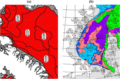
Figure 2. Different ice chart symbols: (a) International egg-symbol, (b) Russian symbol for drifting ice (if multiple ice types), (c) Russian symbol for drifting ice (if single ice type), (d) Russian symbol for fast ice (AARI 2021b). The contents of the symbols are described as per Table 1.

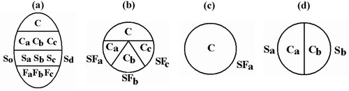
Table 1. Contents of ice chart symbols (AARI 2021b; Canadian Ice Service 2021a).

Symbol	Explanation
$C$	Total concentration of ice in an area (tenths).
$C_a,C_b,C_c$	Partial ice concentrations: concentration of the thickest ice ($C_a$), second thickest ($C_b$), and third thickest ($C_c$).
$S_a,S_b,S_c$	Stage of development of the thickest ($S_a$), second thickest ($S_b$) and third thickest ($S_c$) ice, the concentrations of which are given by $C_a$, $C_b$, and $C_c$, respectively.
$S_0$	Stage of development of ice thicker than $S_a$ but having a concentration of less than 1/10.
$S_d$	Stage of development of any other remaining class
$F_a,F_b,F_c$	Form of ice (floe size) corresponding to $S_a$, $S_b$, and $S_c,$ respectively.
$S{F}_a,S{F}_b,S{F}_c$	Stages of developments combined with a depiction of the form of ice (unique for Russian charts).

Egg code-based Arctic ice charts have some general limitations including the following. First, they include no or limited information on ice ridging and their ice thickness estimates are subject to significant uncertainty (e.g. ‘thick first-year ice’ is defined as any first-year ice thicker than 120 cm). Second, they include no or limited information on the occurrence of pressured ice, which might significantly increase a ship’s resistance and the amount of ice loading acting on its hull. As per Kubat et al. (2012) and Turnbull et al (2019), the occurrence of pressured ice depends on multiple factors, including the speed and direction of the prevailing wind and sea currents, as well as on the presence of shorelines acting as geographical boundaries. Third, they include no information on physical and mechanical ice properties, which as per Timco and Weeks (2010) are needed for detailed ice load calculations.

There are no established guidelines for how to use egg code data when assessing ship operations in ice. Nevertheless, for the purpose of, e.g. transit simulations, the data may be converted to an equivalent thickness. The concept of equivalent ice thickness is based on the assumption that an ice cover with a specific equivalent ice thickness has a similar effect on a ship's performance as level ice of a corresponding thickness. However, as pointed out by Riska (2009), there is no generally accepted definition of equivalent ice thickness, but several competing ones. Nevertheless, as per the same source, a simple definition that based full-scale measurements results in roughly correct values is the average thickness of all the ice in an area. For ice data given in the egg code format, a convenient volume equivalent definition is proposed by Milaković et al. (2018).

It should be noted that the concept of equivalent ice thickness, which effectively averages out local sea ice variations, may not be appropriate for all types of assessments. For instance, for the assessment of a ship’s maximum level of ice loads, depending on the assessment method, the maximum ice thickness in an area might be more relevant than the equivalent ice thickness.

Considering the above highlighted limitations of the egg code, a more precise standard would be welcome. Meanwhile, to compensate for the limitations, the available ice chart data can be supplemented with statistical data on local sea-areas specific ice features, such as ice ridging characteristics, obtained through in-situ measurements and observations. Comprehensive databases containing such statistical data are presented by Romanov (1995) and Dumanskaya (2014). The available ice data can also be supplemented by empirical models of ice growth, such as the Stefan's equation, which describes the dependence between temperature history and ice thickness (Ashton 1986). This approach is practical as reliable satellite-based air temperature records are available for most Arctic regions. To compensate for the lack of information on ice material properties, as per Chai et al. (2021) there are approximate empirically determined relationships between the physical (e.g. temperature history) and the mechanical properties of ice.

2.2. Icebergs

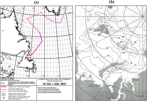
The risk of a collision with an iceberg can be assessed directly based on ice charts or by using a dedicated risk model such as the one presented by Khan et al. (2020). In addition, there are studies on the risk of collisions between icebergs and stationary offshore structures, such as Lu et al. (2019), some of which may also be relevant for ships. For the Canadian Arctic, the Canadian Ice Service (2021b) publishes frequently updated iceberg charts, an example of which is presented in Figure 3. These are prepared mainly based on satellite observations and present the number of observed icebergs per degree square areas, i.e. areas roughly corresponding to 100 × 100 km in size. For the Russian Arctic, the AARI provides statistical data on the size and occurrence of icebergs (Sabodash et al. 2019). In addition, a significant amount of statistical data is presented by Abramov (1996) in terms of contour lines indicating the annual occurrence probability of icebergs in the Arctic sea, examples of which are presented in Figure 3.

Figure 3. (a) Example iceberg chart by Canadian Ice Service (2021b), (b) example of contour lines by Abramov (1996) indicating the annual occurrence probability of icebergs in the Arctic sea.

3. Operational risk management

3.1. POLARIS, Polar Class, and structural risk

This section presents an Arctic shipping operational risk-management framework. The framework is an augmentation of the current Polar Operational Limit Assessment Risk Indexing System (POLARIS) methodology presented in IMO (2016) to model consequences associated with Arctic ship ice damage events. The framework was originally proposed by Browne et al. (2020).

Vessels operating under the Polar Code (IMO 2015) are required to complete risk-based operational assessments to establish vessel operating limits and procedures. The Polar Code recommends the POLARIS methodology for the assessment of risk and assignment of operating limits. POLARIS evaluates the risk of structural damage posed to a ship operating in ice conditions with regards to the vessel’s assigned Polar Class. POLARIS has been shown to well reflect structural risk, but the current methodology does not directly account for the potential consequences that may result from a vessel incurring ice-induced damage (Kujala et al. 2019b).

The overall risk profile of a vessel depends on the magnitude of consequences, should an accident occur. Vessels with higher potential consequences (e.g. life-safety, environmental, or socio-economic) should be operated more conservatively. The framework described in this section supports operational risk management and the assignment of operational criteria based on the likelihood of ice-induced damage and the potential consequences. A detailed description of the accident consequence modelling is provided in chapter 6.

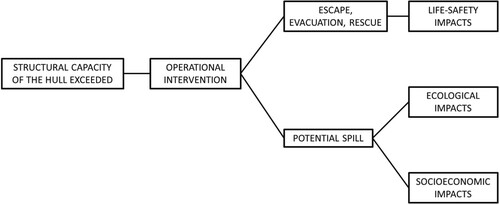
The chain of consequences considered in the risk framework is presented in Figure 4.

Figure 4. The chain of consequences following ice damage to a vessel considering life and environmental safety (Browne et al. 2020).

3.2. A framework for integrating consequences into Arctic shipping risk models

The framework proposes the addition of an operational exposure adjustment term in the current POLARIS methodology that reflects the magnitude of potential consequences. Consequence categories are used to inform the assessment of a vessel’s operational exposure level. The exposure level corresponds to a Risk Index Value (RIV) adjustment factor, which is used to calculate a modified Risk Index Outcome (RIO) that reflects the magnitude of life-safety and environmental risks.

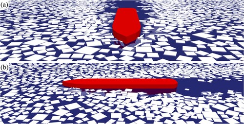
There are eight steps to the framework (Figure 5). The steps are described below.

Figure 5. Procedure of the proposed framework.

Step 1: Life-safety category

The life-safety category reflects exposure in relation to the safety of crew and passengers, should an evacuation occur in Arctic waters. Vessels with a high number of personnel on board (POB) and operations remote from search and rescue infrastructure will pose higher life-safety consequence severity. It is noted that the present search and rescue infrastructure in the Arctic is very limited although it is vital for an appropriate response in case of an accident. A framework to systematically develop SAR in the Arctic is provided by Benz et al. (2021).

Under the proposed framework, scenarios are assigned a life-safety category ranging from minor (S1) to disastrous (S5), as per Table 2. A scenario-based life-safety consequence model for Arctic ship evacuations (Browne et al. 2021) is described in Section 6.1.

Table 2. Life-safety categories.

Life-safety category	Assigned Value
Disastrous	S5
Catastrophic	S4
Significant	S3
Severe	S2
Minor	S1

Step 2: Ecological sensitivity category

The ecological sensitivity of a geographic region is evaluated through ecological risk assessments and marine environmental assessments. Different approaches for defining ecological sensitivity exist in the literature, and typically include one of the following:

• Protected areas and other valuable areas

• Threatened species and habitats

• Other species and habitats sensitive to oil

The Area Risk Assessment (ARA) methodology of Transport Canada, presented by Dillon Consulting (2017), is an existing approach that may be applied to evaluate ecological sensitivity. The ARA methodology uses a five-point sensitivity index. The highest sensitivity scores are for protected areas and species that have legislated status. Under the proposed framework, regions are assigned an ecological sensitivity category (E), ranging from minor to very high as per Table 3.

Table 3. Ecological sensitivity categories.

Ecological Sensitivity Category	Assigned Value
Very high	E = 5
High	E = 4
Medium high	E = 3
Moderate	E = 2
Minor	E = 1

Applying any indexing system to evaluate ecological sensitivity requires spatial data on relevant ecological features (e.g. on protected areas). Such data are provided by for instance AMAP/CAFF/SDWG (2013).

Step 3: Socio-economic protection category

The socio-economic value of a region is evaluated through the assessment of different socio-economic indicators. Indicators are grouped based on common objectives. Examples of socio-economic indicator groups include those defined in the draft Nunavut Land Use Plan (Nunavut Planning Commission 2016):

• Protecting and sustaining the environment

• Encouraging conservation planning

• Building healthier communities

• Encouraging sustainable economic development

Under the proposed framework, regions are assigned a socio-economic protection category (P) based on the number of indicator groups identified for a region. A higher number of indicator groups corresponds to a higher protection status. Protection categories reflect the socio-economic value of the region, ranging from minor to very high as per Table 4.

Table 4. Socio-economic protection categories.

Protection Status	Assigned Value
Very high	P = 5
High	P = 4
Medium high	P = 3
Moderate	P = 2
Minor	P = 1

Step 4: Spill consequence category

The spill risk for a vessel will depend on the amount and type of potential contaminant carried on board. Through oil spill risk assessments, vessels could be identified as having high, moderate, or minor levels of potential spill consequence (SC), as presented in Table 5.

Table 5. Spill consequence categories for vessels.

Spill Consequence	Assigned Value
High	SC = 3
Moderate	SC = 2
Minor	SC = 1

Step 5: Protection status, ecological sensitivity, and spill consequence index (PESCI)

An overall environmental consequence category is assigned. The process is referred to as the Protection Status, Ecological Sensitivity, and Spill Consequence Index (PESCI) method. A PESCI value is dependent on the socio-economic protection status (P) and ecological sensitivity (E) categories for the region, and the spill consequence category (SC) for the vessel. Notional PESCI values are assigned in accordance with Table 6 a, b, and c, which correspond to spill consequence categories (SC) of 1, 2, and 3, respectively.

Table 6. PESCI values.

P	5	4	5	6	7	8	P	5	5	6	7	8	9	P	5	6	7	8	9	10
	4	3	4	5	6	7		4	4	5	6	7	8		4	5	6	7	8	9
	3	2	3	4	5	6		3	3	4	5	6	7		3	4	5	6	7	8
	2	1	2	3	4	5		2	2	3	4	5	6		2	3	4	5	6	7
	1	0	1	2	3	4		1	1	2	3	4	5		1	2	3	4	5	6
		1	2	3	4	5			1	2	3	4	5			1	2	3	4	5
		E							E							E
a. PESCI values (SC = 1)							b. PESCI values (SC = 2)							c. PESCI values (SC = 3)

The PESCI value corresponds to the overall environmental consequence category, ranging from minor (C1) to very high (C5), in accordance with Table 7.

Table 7. Environmental consequence categories.

Environmental Consequence Category	PESCI Range
C5: very high consequence	PESCI > 7
C4: high consequence	5 < PESCI ≤ 7
C3: medium high consequence	3 < PESCI ≤ 5
C2: moderate consequence	1 < PESCI ≤ 3
C1: minor consequence	PESCI ≤ 1

Step 6: Operational exposure level

The environmental consequence category and life-safety category are combined to inform the operational exposure level. Notional values are provided in Table 8.

Table 8. Operational exposure levels.

Life-safety Category	S5 (disastrous)	L5	L5	L5	L5	L5
	S4 (catastrophic)	L4	L5	L5	L5	L5
	S3 (significant)	L3	L4	L5	L5	L5
	S2 (severe)	L2	L3	L4	L5	L5
	S1 (minor)	L1	L2	L3	L4	L5
		C1 (minor)	C2 (moderate)	C3 (medium high)	C4 (high)	C5 (very high)
		Environmental Consequence Category

Step 7: Risk index value (RIV) adjustment for operational exposure level

The operational exposure level is incorporated in the current POLARIS methodology through adjustment of the calculated RIVs. Notional RIV adjustment factors corresponding to operational exposure levels are presented in Table 9.

Table 9. Risk Index Value (RIV) adjustment factors for operational exposure levels.

Operational Exposure Level	RIV Adjustment Factor
L5	RIVL5 = −2.0
L4	RIVL4 = −1.5
L3	RIVL3 = −1.0
L2	RIVL2 = −0.5
L1	RIVL1 = 0

Step 8: Modified risk index outcome (RIO)

Using the RIV adjustment factor, a modified RIO is calculated following Equation (1) (1) $\begin{array}{rl}\mathrm{R}\mathrm{I}{\mathrm{O}}_{\mathrm{m}\mathrm{o}\mathrm{d}\mathrm{i}\mathrm{f}\mathrm{i}\mathrm{e}\mathrm{d}}=& C_1\times \left(\mathrm{R}\mathrm{I}{\mathrm{V}}_1+\mathrm{R}\mathrm{I}{\mathrm{V}}_{\mathrm{L}}\right)+C_2\\ & \times \left(\mathrm{R}\mathrm{I}{\mathrm{V}}_2+\mathrm{R}\mathrm{I}{\mathrm{V}}_{\mathrm{L}}\right)+\cdots +C_n\\ & \times \left(\mathrm{R}\mathrm{I}{\mathrm{V}}_n+\mathrm{R}\mathrm{I}{\mathrm{V}}_{\mathrm{L}}\right)\end{array}$(1) where C₁ … C_n is concentration (in tenths) of each ice type within the ice regime, RIV₁ … RIV_n is the corresponding standard RIVs for each ice type (following POLARIS); and RIV_L is the RIV adjustment factor.

The modified RIO is then used to inform risk-based operating criteria, as per the current POLARIS methodology: ‘Normal’, ‘Elevated operational risk’, or ‘Operations subject to special consideration’.

3.3. Illustrative example

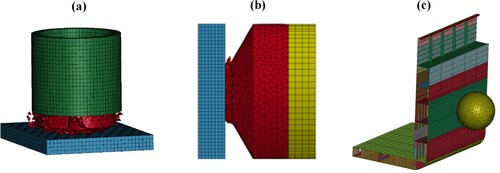
An illustrative example presented in Figure 6 demonstrates the assignment of operating criteria following the current POLARIS methodology and the proposed operational risk management framework. POLARIS recommends ‘Normal Operations’. Through consideration of potential consequences and the vessel’s operational exposure level, the proposed risk management framework recommends ‘Elevated Operational Risk’.

Figure 6. Illustrative example.

3.4. Limitations and future work

A framework has been proposed for the purpose of distinguishing and integrating consequence severities into Arctic shipping operational risk models and to support more holistic risk-based decision making. Life-safety, ecological, and socio-economic consequence categories (Steps 1–3) are based on empirical evidence and established methodologies. The notional values presented in Steps 4–8 require further development and negotiation. Future work includes refining consequence models, developing consequence aggregation methods, collecting stakeholder feedback, and validating the efficacy of operational risk mitigation strategies.

The proposed framework is applied through augmentation of the POLARIS methodology. Several limitations and areas for future work are acknowledged. Regarding the modification of POLARIS, it is acknowledged that RIV adjustment factors and additional case studies require further investigation and debate.

POLARIS provides an indication of the risk of structural damage from ice based on a vessel’s ice class and the prevailing ice conditions. The proposed approach does not challenge the structural risk assessment inherent in POLARIS. Rather, the intent of the proposed approach is to provide a mechanism to consider life-safety, ecological, and socio-economic consequences in the operational risk management of Arctic shipping. Further, applying the framework to POLARIS links the potential consequences of Arctic ship accidents solely to ice damage. Other accident types, for instance, groundings, should be considered.

POLARIS is used by ship captains and officers to support decision-making during voyage planning and navigation, and by ship owners, classification societies, and insurance underwriters to communicate expectations for safe operations and risk management (Fedi et al. 2018). Any proposed augmentation of POLARIS must be easily understood and usable by practitioners. To support the integration of consequences in the POLARIS methodology, RIV adjustment factors may be predetermined for a given ship type, ice class, and operating region. On board software could support calculation of modified RIO values and assignment of operating criteria.

Finally, the Polar Code, SOLAS, MARPOL, and the International Convention on Standards of Training, Certification, and Watchingkeeping for Seafarers (STCW) differentiate risk associated with different ship types. Incorporating life-safety, ecological, and socio-economic consequences into operational risk management practices requires consideration of the existing network of regulations governing Arctic shipping.

4. Ice load assessment

4.1. General

As explained above, POLARIS provides an indication of the risk of structural damage from ice based on a vessel’s ice class and the prevailing ice conditions. However, it should be noted that POLARIS assesses risk in terms of a non-dimensional risk index. To assess the actual safety of a ship with regards to ice loading, the anticipated ice loads must be calculated. As per Kujala et al. (2019a), available methods for this purpose can be divided into three main categories:

• Theoretical or first-principle methods, which are methods that have a theoretical core supported by empirical features. Such methods can be further divided into analytical (exact) and numerical (approximate) methods.

• Semi-empirical methods, which are methods that have an empirical core, typically based on full-scale hull ice load measurements, supported by theoretical features making them applicable to a range of ship designs (e.g. ships with different hull angles).

• Empirical methods based on direct or indirect full-scale ice load measurements.

The choice of method for a specific assessment depends on multiple factors, including the specific objectives and criteria of the assessment, as well as the availability of time, resources, and input data.

A common challenge of theoretical or first-principle methods is that they require an assumption of how ice fails when interacting with a ship’s hull (Tunik 1991). This is challenging because the way in which ice fails, often referred to as the failure mode, depends on multiple dynamic and partially unknown factors including the relative velocity between the ice and impacting ship, the contact geometry between the hull and the ice, the spatial–temporal variation of the contact stresses, and the ice strength (ISO 2010; Timco and Weeks 2010). Uncertainties associated with these factors translate into significant uncertainty in the obtained ice load estimate (Riska 2019).

A common challenge of empirical and semi-empirical methods, on the other hand, is their dependency on relevant full-scale ice load measurements. In general, for such data to be relevant for a specific ship, it should have been measured on a ship of approximately similar size, hull shape, and operation conditions. As per Kendrick and Daley (2011) and Suominen (2018), multiple full-scale ice load measurement campaigns have been carried out over the years. Nevertheless, because full-scale ice load measurements are expensive, the available data still covers only a limited range of vessel designs and operating scenarios. Another common limitation of empirical and semi-empirical methods is that they do not consider human factors. This is significant as the loads that a ship experiences may be significantly influenced by the actions taken by its crew (Daley et al. 1991; Billard et al. 2014; Valtonen 2016).

As indicated above, at present practically all known methods for assessing ship-ice interactions suffer from uncertainties relating to a lack of relevant input and validation data. This derives from the fact that there are significant challenges related to full-scale measurements of the ice cover through which a ship passes, the ship-ice interaction process, and the related structural loads.

As explained by Kujala et al. (2019b), state-of-the-art approaches for full-scale ice load measurements on ships involve the use of stereo cameras for observing ice thickness and strain gauges for indirect measurement of ice loads in combination with FEM-based structural analysis. A significant limitation of direct measurements is that they do not enable measurements of local pressure variations within an individual hull panel. However, presently there is no feasible alternative as there is no readily available approach for direct long-term measurements of ice-induced pressures on realistic hull shapes.

Ice charts do not provide detailed enough data to make it possible to link the ice condition that a ship encounters and the resulting ice load measurements. Thus, to be able to link the two, ice load measurements must be combined with onboard ice condition monitoring. As per above, the use of stereo cameras has proven somewhat effective. Towards a more systematic and accurate approach, Sandru et al. (2020) present a system for automatic ship-borne ice-field analysis. Utilizing machine vision cameras in combination with inertial and satellite positioning sensors, the approach promises to enable automated acquisition of data on sea ice concentration, ice floe size, and ice floe distribution. A similar system is proposed by Sandru et al. (2021), which instead of using machine vision cameras uses the Light Detection and Ranging (LiDAR) method.

In comparison with LiDAR, machine vision cameras are less expensive and enable monitoring of a larger area with a width of 200–300 m (Sandru et al. 2020). Using LiDAR, the maximum size of the monitored areas depends on the type of LiDAR used. Relatively inexpensive off-the-shelf devices can cover an approximately 60 m wide area, whereas more customized and expensive devices may enable monitoring of larger areas (Sandru et al. 2021).

Machine vision cameras can provide 2D spatial information at a very high frame rate, which is useful when monitoring ice conditions. Through processing, the 2D information can be extracted into a 3D format. LiDAR, on the other hand, provides more accurate 3D spatial measurements directly in the form of point clouds with an error margin of ±2.5 cm. Because the measurements are in the form of point clouds, they can be used both to measure ice thickness and to detect individual ice features such as ice ridges.

A quite significant drawback of machine vision cameras is that they do not work in low visibility conditions such as rain, fog, or snow. In addition, in darkness they only work if artificial light is provided, e.g. by the ship’s searchlights. LiDAR, on the other hand, is not dependent on daylight and the effects of rain and snow can be filtered out using algorithms. Thus, both machine vision cameras and LiDAR have their advantages and drawbacks, but together they complement each other.

4.2. Analytical methods

As per Riska (2018), the design loads behind both the Polar Class and the Russian ice class regulations (RS 2019) are calculated using the so-called Popov method that was originally presented by Popov et al. (1967) and later further developed by Daley (1999). In comparison with numerical and semi-empirical methods, a major strength of the method is that it is fundamentally analytical as it is based on the laws of conservation of energy and momentum in collisions. As used in the Polar Class rules, the method reduces a sliding-oblique collision between a ship and an ice floe, which represents a three-dimensional physical problem, to an equivalent one-dimensional mathematical model.

As per Daley (1999) the method requires three categories of input:

• Ice indentation pressure. To solve the general energy equations, it is necessary to formulate an equation that relates pressure to indentation. It is assumed that the ice pressure depends on the indentation so that the maximum pressure arises at the time of maximum penetration.

• Geometric and kinematic properties of the involved ship and ice.

• The effect of the surrounding water corresponding to its hydrodynamically added mass.

A limitation of the method is that it may not to support highly detailed simulations as it assumes a constant ice pressure over the hull-ice contact area. Also, as shown in Idrissova et al. (2019), ice loads calculated by the Popov method are sensitive to variations in the input parameters. Thus, as when using any other ice load assessment method, careful attention should be paid to the definition of the ship-ice collision scenario, the ship-ice contact geometry, and the ice conditions, among other input parameters.

It is noted that as per Lu et al. (2020), energy-based methods similar to the Popov method could potentially also be used to assess loads in ship-iceberg collisions.

4.3. Numerical methods

The ship-ice interaction process, due to its dynamic, non-linear, three-dimensional, and multi-physical nature, is highly complex. As a result, using numerical models for the calculation of ice loads on ships is challenging, although feasible.

The ship-ice interaction process is affected by the geometry and velocity of the ship, the dimensions and failure process of the ice feature, and the surrounding water. A detailed simulation of the involved processes is computationally heavy, and further complicated by the fact that the mechanics of the interaction process are not fully understood yet. Nevertheless, different simulation approaches have been developed. One approach is to simplify the involved physics sufficiently enough to make a numerical simulation of a ship advancing in ice over a limited distance computationally manageable. This approach is well-suited for gaining insights on the relationships between ice loads and ice conditions, as well as on the distribution of ice loads over a given period. While this approach allows simulations of extensive interaction processes, the trade-off is that the simulations do not yield sufficiently detailed information on, for instance, the distribution of local ice pressures. It is also clear that the reliability of any simulation of this kind is strongly dependent on the generalizations that have been made. Simplified models may not be able to capture the essential mechanics in the ship-ice interaction, which sets strict requirements for model validation.

Another approach is to aim for detailed modelling of individual ice-ship hull contacts. Such models with a high spatial and temporal resolution can provide insights on contact pressure distributions and the interaction between fragmenting ice and a deforming hull structure. However, a high resolution comes with a computational burden, which sets restrictions, e.g. in terms of the maximum feasible spatial and temporal extent of a simulation.

Considering the above, there is no one recommended practice concerning the use of numerical models for calculating ice loads. Instead, a suitable numerical modelling approach must be selected considering the problem at hand. Approaches capable of simulating ship-ice interaction on large spatial and temporal scales can be used to study, for example, ice load statistics. Approaches capable of detailed analysis of ice fragmentation, on the other hand, can be used to study ice pressure distributions on a ship hull. Thus, the two approaches can be complementary, as knowledge obtained from detailed small-scale simulations can be parameterized and used to increase the accuracy of larger-scale simulations.

It is paramount to validate any numerical model used for the simulation of ice loads. Validation can be done by comparing the numerical results with corresponding full- or model-scale (ice tank) measurements, but it is important to consider both the spatial and temporal scale used in the validation.

A general challenge when comparing load statistics, especially in the case of model scale data, is that all experimental data cover a limited time span and a limited set of ice conditions. On the other hand, a major advantage of model scale experiments is that all the parameters and boundary conditions are known, which makes the comparison of individual load events simpler than if the verification data originated from full-scale tests.

For the simulation of ice loads, there are two primary numerical methods, namely the Discrete Element Method (DEM) and the Finite Element Method (FEM). In general, DEM and FEM simulations can be considered complementary: DEM simulations can be used to find ice load distributions, to detect the areas of a ship hull that are exposed to the highest ice loads, and to estimate ice load magnitudes under given ice conditions. FEM simulations, on the other hand, can be used to produce ice pressure distributions corresponding to ice loads from DEM simulations and to study, for example, the effects of hull deformation. In the following, these two different methods are addressed in greater detail.

4.3.1. Discrete element method

Most, if not all, ship-ice interaction scenarios include interactions of discrete ice blocks. A ship may break ice pieces off an intact ice sheet and this process defines the ice load. Once broken off, an ice block may slide along the ship hull and further affect the ice loading process. Another important loading scenario is the interaction between a ship hull and ice floes in sea areas with partial ice concentration. For this scenario, the related processes can be simulated using the discrete element method (DEM) by Cundall and Strack (1979), which, as per Tuhkuri and Polojärvi (2018), has been applied to ice mechanics since the mid-1980s (Williams et al. 1986; Hopkins 1992). In ice mechanics, a typical DEM simulation consists of hundreds or thousands of interacting ice features. The simulations are explicit and advance in short time steps, the ice blocks are assumed rigid, and contact forces are solved by using models mimicking the effects of contact deformation. On a given time step, the contact forces and external forces acting on each block are solved. Newton’s second law is used to determine the accelerations, and a numerical integration scheme of choice is used to update the velocities and positions of each block. Implicit, non-smooth, or event-driven, DEM simulations have also been used (Metrikin and Løset 2013; van den Berg et al. 2018).

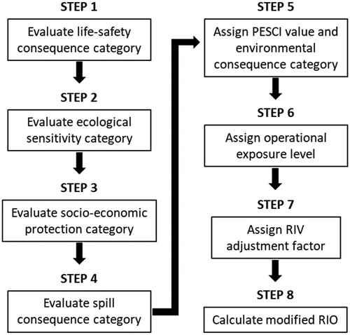
DEM has been used to simulate ships breaking level ice, but because such simulations are computationally intensive, either only very small domains have been simulated, or the failure process has been pre-defined or simplified (Lubbad and Løset 2011). To date, no simulation of ships breaking level ice using a rigorous model of the ice field fragmentation has been conducted. The simulation of ships navigating through ice floe fields is computationally easier (Metrikin and Løset 2013; van den Berg et al. 2020; Yang et al. 2021). However, most studies, regardless of whether they considered level ice or ice floe fields, have concentrated on ice resistance rather than local loads (Polojärvi et al. 2021a, 2021b). Anyhow, through DEM simulations it is also possible to both generate simulated ice load data, as well as to study the distribution of ice loads on a ship’s hull. In addition, validated DEM simulations make it possible to study, in a controlled manner, how a ship’s ice loads depend on individual ice parameters, such as floe size and coverage. Examples of such studies are given in Figures 7 and 8. Corresponding studies in model-scale would be highly laborious and expensive, and in full-scale such studies would not be feasible as it would practically not be possible to control the measurement conditions with sufficient precision.

Figure 7. Snapshot from a simulation with ice floe field consisting of 14,329 rectangular floes of size 5 … 15 m and thickness 0.5 m. The floe field has an ice concentration of 50% and its dimensions are 0.5 km × 2.0 km. The ship is moving with a constant velocity of 1 m/s. Figure reproduced from Polojärvi et al. (2021b).

Figure 8. Simulation snapshots from (a) the front and (b) the side of the showing rotated and rafted, 0.5 m thick, ice floes around the ship hull and the open channel behind the ship. Figure reproduced from Polojärvi et al. (2021b).

While DEM simulations have provided important input for ship-ice and ice-structure interaction studies, some challenges and limitations exist. First, future research is needed to enable a reliable simulation of the hydrodynamics related to ship-ice interaction. Obtaining a fully coupled and detailed CFD-DEM solver enabling extensive simulations of ships operating in ice over a period of tens of minutes appears a major challenge. To overcome this challenge, future research should concentrate on new ways to simplify the related hydrodynamics while maintaining a sufficient level of accuracy and reliability. Second, while ship interactions with pressure ridges have been successfully simulated using DEM, see Gong et al. (2019), more data on the properties of the consolidated layer of ridges is required to make it possible to fully model the process of a ship penetrating through an ice ridge. Third, sophisticated contact models, including ice pressure distributions, could be integrated into DEM models. Fourth, the use of multiscale models could be explored, in which a high-resolution model for contact interface would be coupled with a coarser resolution model for the rest of the domain.

4.3.2. Finite element method

As per Nowacki (2010), the finite element method (FEM) represents the state-of-the-art in structural design. In recent years, the potential use of FEM for the simulation of ship-ice interactions has been a significant topic of research (see e.g. Kim et al. 2015; Yu et al. 2021). Arguments in favour of using FEM include the method’s maturity and accuracy in solving continuum mechanics problems. In addition, commercial solvers such as LS-Dyna or Abaqus explicit are well suited to handle large structural models and complex contact problems.

In the context of ice-hull interaction analysis, potential applications of FEM include the analysis of hull structural response and strength characteristics, either of new or existing designs, with the aim to determine appropriate operational limitations or to access the consequences of potential accidental impacts.

In general, there are three different main approaches to consider ice loads in FEM-based models:

• Non-coupled pressure mapping approaches: In these approaches, ice loads are modelled in terms of predetermined pressures corresponding to the considered design load cases (e.g. as specified by class rules or empirical pressure-area relationships). The pressures are mapped onto the structure being analysed. This approach is numerically cheap and robust, making it the industrial standard in structural design. However, this concept does not take into account the interaction between the ice load and the resulting structural response (Quinton et al. 2012). As a result, depending on the applied load assumptions, there is a risk of obtaining flawed structural failure modes. Since there is no coupling between the interacting ice and ship structure, the approach is not well suited for the simulation of large plastic deformations or structural failure. Ice rules and common pressure-area based approaches assume constant ice pressures, as a result of which spatial and temporal varying High-Pressure Zones, which are typical for brittle ice loads (Gagnon et al. 2020; Herrnring et al. 2020), are neglected. As per Erceg et al. (2014), this may result in non-conservative assessments of the structural safety of hull structures.

• Fully-coupled approaches: In fully-coupled approaches, the ice feature and ship structure are solved in a single FE model to achieve a detailed representation of the involved ice forces and pressures. This requires finding a suitable ice model for the considered problem. This is challenging as the mechanical behaviour and many of the processes related to the ice-structure interactions occur very locally and are not fully understood, as demonstrated e.g. by Jordaan (2001) and Browne et al. (2013). Fracture and continuums mechanic processes occur simultaneously, resulting in a global weakening of the ice. In addition, locally hardening effects have been observed. Several ice models for fully-coupled simulations have been presented, including crushable foam models, see Gagnon (2011) and Kim et al. (2015), and plasticity-based iceberg models, see Liu et al. (2011) and Yu and Amdahl (2021). Iceberg material models do not apply to typical ice collision scenarios because splitting and spalling of the contact interface are not considered. Both effects are important for the development of High-Pressure Zones, which are present in typical ice-structure interaction scenarios. Since the ice and the structural problem are solved in a single model, simulations of large structural deformations, including structural failures, are possible. Thus, fully coupled models have the potential to be both versatile and accurate. A general open question related to these and other FEM models is the treatment of ice failures. The ice failure process is often modelled using the element erosion technique. However, if this approach is used to simulate ice failure under compression, element erosion results in unphysical behaviour as the actual ability to transmit loads in the contact zone is lost. In addition, the elemental erosion technique violates the conservation of mass and energy.

• Weakly-coupled approaches: Weakly-coupled simulations represent an intermediate solution between non-coupled and fully coupled approaches. In these approaches, ice loads are idealized and computed during a simulation by a separate ice model. In general, ice forces and pressures are determined based on pressure-area relationships in combination with equations of motions or the Popov method (Popov et al. 1967). An example of a weakly-coupled model is presented by Kolari and Kurkela (2012). Potential applications include analyses of ship-ice floe or ship-iceberg collisions. Since these approaches mostly assume constant ice pressures, they are subject to the above-mentioned disadvantages of pressure mapping approaches. In addition, because these approaches typically apply a highly idealized ice-load model, they are not well-suited to handle large plastic deformations or structural failures.

To avoid the above-mentioned issues of the element erosion technique, Herrnring and Ehlers (2021) present the Mohr Coulomb Nodal Split (MCNS) ice model. To date, the MCNS model has been validated for crushing and spalling dominated problems. Application to flexural failure dominated problems is also possible. However, it must be decided on a case-by-case basis whether some fracture mechanic concept, such as Cohesive Zone Method (CZM), would be better suited (Kellner et al. 2021).

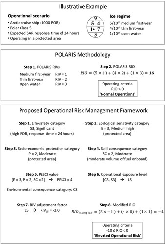
The MCNS model enables geometric change due to fragmentation, material transport and is at low confinement rations almost energy- and mass preserving. Failure is represented by a node splitting approach. Failed elements are simply detached and remain in the simulation. For a variety of complex crushing dominated problems, the numerical results demonstrate good agreement with corresponding full-scale measurements. Examples of validated simulations are shown in Figure 9(a,b). We also plan to consider ship- growler collisions as visualized in Figure 9(c). The impact scenario showed in Figure 9(c) represents an idealized case where a growler hits the side of a ship. More probable and realistic ship-growler impacts scenarios will be considered in the future. Among others, we aim to investigate the role of the shape of an impacting growler on the resulting structural loads and responses.

Figure 9. Examples of FEM-based simulations of ice-structure interactions: (a) a MCNS simulation of an ice-extrusion test (Herrnring and Ehlers 2021), (b) a MCNS simulation of a double pendulum test (Herrnring and Ehlers 2021), and (c) simulation of an idealized collision between a ship's hull side and a grawler.

In summary, FEM represents a powerful tool for the simulation of ice-structure interactions. There are multiple different FEM-based approaches to assess ice loads, suitable for different scenarios. Non-coupled pressure mapping approaches represent the industrial standard and are applied in ice class regulations, among others. However, as explained above, these approaches are associated with limitations that the user must be aware of. In recent years, significant research efforts have been made to advance the development of different types of coupled methods. However, due to related technical challenges, no technical standard has yet been obtained. As a result, engineers must assess on a case-by-case basis and based on extensive validations, what ice model is the most suitable. Further research is needed for improved scalability, accuracy, and robustness.

4.4. Semi-empirical approaches

4.4.1. Event-maximum method

As demonstrated by Jordaan (1987), Daley et al. (1991), Kujala (1996), among others, ice loads have a stochastic nature. Consequently, a ship's expected long-term extreme ice load depends not only on the worst ice conditions that it is expected to encounter, but also on the extent to which it is expected to operate in those and other ice conditions. A limitation of the Polar Class rules, and thus also POLARIS, is that they do not take this aspect into account. To address this limitation, i.e. to assess whether there is a risk that a ship's design load (e.g. as determined in accordance with its Polar Class) will be exceeded in the long run, designers may apply a probabilistic semi-empirical method based on Jordaan et al. (1993) known as the event-maximum method.

The event-maximum method was originally intended primarily for application to offshore structures and is referred to in the ISO 19906:2010 standard for offshore structures (ISO 2010). Nevertheless, as demonstrated by Taylor et al. (2010), the method can also be applied to ships, e.g., to estimate for a specific hull area the relationship between the area's maximum ice pressure and ice exposure, quantified in terms of the number of interactions with different types of ice.

Using a modified version of the method by Shamaei et al. (2020), the long-term maximum loads associated with a ship's individual operating profile can be calculated in terms of a line load (e.g. kN / m) along its hull-ice interface. As proposed and demonstrated by Bergström et al. (2022), the modified version can be used as a supplement to POLARIS when selecting a ship's polar class. However, in line with section 4.1, due to its semi-empirical nature, the method has fundamental limitations that must be acknowledged and considered. Further research is recommended to address these. Specifically, it is recommended that future theoretical properties be added to the model to make it more generalized. Recent advances in this regard include Li et al. (2021).

4.4.2. Other semi-empirical approaches

In addition to the event-maximum approach, there is a range of other semi-empirical methods to calculate ice loads, most of which are based on full-scale datasets fitted to different types of distributions. The general principle of these methods is that the distribution of ice loads measured on a ship over a period can be assumed to depend on factors such as the ship's design, speed, and operating conditions (e.g. ice thickness, ice concentration and flake size), and that the parameters of such ice load distributions can be modelled as functions of those. Different statistical modelling approaches have been considered in the literature, including exponential and lognormal distributions, Weibull distributions, generalized probability distributions based on kernel density estimations, combinations of different exponential models, as well as average conditional exceedance rate functions (Kujala et al. 2019a).

Using a hierarchical Bayesian model of the same type often used in machine learning, Kotilainen et al. (2017, 2018, 2019) made an attempt to establish quantitative relationships between a given set of ice condition parameters and a corresponding set of ice load distribution parameters. The outcomes of the resulting model agree well with validation data, which indicates that it is feasible to establish mathematical relationships between distributions of ice load measurements and different ice condition parameters. Nevertheless, the results of any such purely mathematics-based models have proven sensitive to the measurement data used to train them.

For estimating extreme values over a specific period, extreme value distributions such as Gumbel I and III have been shown to give the best fit. Kujala (1994) presented an early attempt to link long-term ice loads with the prevailing ice conditions based on 12-hour maximum load values measured in Baltic Sea ice conditions and Gumbel I parameters. Later this approach was also applied to full-scale ice load measurement data recorded on S.A. Agulhas II in the Southern Ocean (Kujala et al. 2019a). However, none of these studies have established a clear link between ship parameters (e.g. engine power and hull shape), ice load distribution parameters, and the prevailing ice condition. Therefore, like with other semi-empirical approaches, the application of these approaches remains limited to ships for which relevant full-scale ice load measurements are available.

4.5. Concluding remarks

As per the above, different ice load assessment methods are suitable for different types of assessments. However, presently all methods have significant limitations, most of which relates to a general lack of relevant input and validation data. This is due to significant challenges related to full-scale ice load measurements, in particular related to the linking of ice loads and ice conditions.

Future research to address the present limitations is well motivated, not the least because new and improved ice load assessment approaches may provide a path towards goal-based hull structural design and regulatory approval, making it possible to tailor a ship's level of ice strengthening to its individual operating area and profile. Potentially, this may result in enhanced maritime safety as well as significant savings in emissions and costs over the lifetime of a ship.

It should be noted that in particular the development of new and improved technologies for real-time monitoring of ice conditions and loads would in addition support the development of situational awareness tools to help ship operators to control ice loads through manoeuvring and other active measures.

5. Hull structural response and design

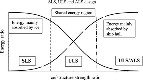
5.1. Structural limit states

Presently, design ice loads for Arctic ship are determined based on design ship-ice interaction scenarios as specified by the ice class rules without any clearly defined return periods (Riska and Bridges 2019). As a step toward a more rational risk-based approach, appropriate structural limit states and probabilistic acceptance criteria should be developed. As starting point, the following limit states as specified by the ISO 19906: 2010 standard for offshore structures should be considered (ISO 2010):

• Serviceability Limit State (SLS), which correspond to criteria governing normal functional use.

• Ultimate Limit State (ULS), which correspond to resistance to extreme ice loads.

• Abnormal/Accidental Limit State (ALS), which corresponds to accidental events.

ISO 19906:2010 also determines a Fatigue Limit State (FLS) to account for the accumulated effect of repetitive loads. Whether or not fatigue must be considered in the context of ice loads on a ship requires further investigations (LR 2011).

Figure 10 indicates, for different limit states, the ratio between the amount of energy absorbed by a ship's hull structure and the energy absorbed by the impacting ice, i.e. the energy ratio. According to the figure, at SLS, the impact energy is mainly absorbed by the affected ice, whereas at ULS and ALS, most of the impact energy is absorbed by the structure. The total impact energy in a ship-ice interaction can be calculated as the sum of areas between the curves.

Figure 10. Different design regions: ULS, shared, and ALS. The vertical axis indicates the ratio between the energy absorbed by the structure and that absorbed by the impacting ice feature.

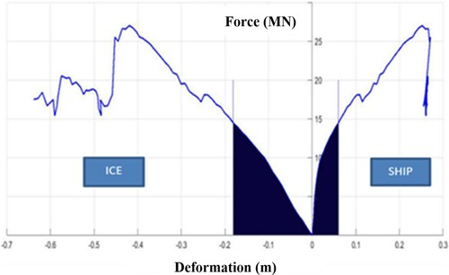
Examples of the numerically simulated structural damages related to ULS and ALS are presented in Figure 11. Figure 12 presents an example of how the impact energy in a ship-ice impact is absorbed by the ice and the structure as a function of the deformation.

Figure 11. Examples of simulated damage resulting from a ship-ice floe/ridge impact: (a) ULS/ALS type of damage (b) ALS type of damage (Radhakrishnan 2018).

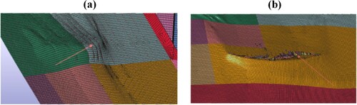
Figure 12. Example energy absorption and load-displacement curve for a ship-ice impact (Radhakrishnan 2018).

5.2. Ice strengthening design using non-linear FEM

The Polar Class rules intend that a hull structure may yield under the design load, but that it should have a substantial reserve against collapse and rupture (Daley 2002; Kõrgesaar et al. 2018). To this end, the rules prescribe minimum scantlings through a set of structural formulae that are determined based on a design load representing a rare event in which a ship strikes an ice edge resulting in a high load (Daley et al. 2001; Daley 2002). The local framing design is based on an idealized plastic collapse onset mechanism (IACS 2016). However, because the IACS has not reached an agreement over the design criteria for large primary structural members (such as transverse web frames), the rules require the strength of those structures to be assessed using either linear or non-linear direct calculation methods, such as the finite element method (Moakler 2018). Because such direct calculations are time consuming, this is problematic especially in the conceptual design phase. Therefore, to make the conceptual design process more efficient, in the following an approach based on closed-form expressions that can be used to define reasonable scantlings for the primary structural members, is proposed. The proposed approach is validated by numerical finite element simulations for five different Polar Classes, namely PC3, PC4, PC5, PC6, and PC7, and three different ice-strengthened hull areas, namely bow, midbody, and stern. Although the validation is limited to PC3-PC7, the approach applies to higher ice classes as well.

The validation case study is carried out based on the main dimensions of the South African icebreaking polar supply and research vessel S.A. Agulhas II, presented in Table 10. The plate and frames are designed according to the Polar Class rules. As per the proposed approach, larger structural members, on the other hand, are designed following the closed-form expressions defined by the Finnish-Swedish Ice Class Rules (FSICR) (Trafi 2017) but with modified safety factors. Specifically, the webframes and stringers are dimensioned to comply with section moduli and shear area requirement calculated using safety factors (f₇, f₈, f₁₂, f₁₃  = 1) instead of the values proposed by the FSICR (f₇ = 1.8, f₈ = 1.2, f₁₂ = 1.8, f₁₃ = 1.1). The goal of this modification is to reduce the mismatch between design philosophies where frames are designed according to the three-hinge mechanism as per the PC rules, whereas the primary members are intended to remain elastic under the design load as per the FSICR rules.

Table 10. Main characteristics of the case study ship S.A. Agulhas II.

Length	134 m
Breadth	22 m
Draft	7.65 m
Deadweight	4780 ton
Displacement	13687 ton
Power	12000 kW
Framing	Transverse
Frame spacing	0.4 m
Stringer spacing	1.5 m
Webframe spacing	2.4 m
Webframe span	6 m
Yield strength of the material	355 MPa
Upper ice waterline angle α (bow)	19 deg
Buttock angle γ (bow)	65 deg
Normal frame angle at upper ice waterline β’ (bow)	12 deg

The load-carrying capacity of the obtained structures as determined by the proposed approach is presented in Table 11. The calculations were carried out using non-linear finite element simulations following ABS guidance notes. Accordingly, the FE simulations were performed with 5-bay grillage models subjected to linearly increasing pressure on a load patch defined as per the Polar Class rules (dimensions depend on the Polar Class class).

Table 11. Calculated structural scantlings per ice class and hull region.

	PC3			PC4			PC5			PC6			PC7
	Bow	Mid	Stern	Bow	Mid	Stern	Bow	Mid	Stern	Bow	Mid	Stern	Bow	Mid	Stern
Frames and plate
t (plate)	26.4	21.4	23	22.4	18.5	19.2	20	15.8	15.8	18.4	13	12.3	17	11.9	10.8
Designs
Z [cm3]	3035.9	371.1	674.6	1980	342.2	229.1	1092.5	135.5	135.5	904.5	109.4	109.4	542.2	45.4	128
A [cm2]	78.1	29.8	36.3	58.7	27.2	26.7	41.5	21.6	21.6	37.8	17	17	30.7	14.7	15.1
web height × thickness [mm]	571 × 17	352 × 12	389 × 13	495 × 15	337 × 11	334 × 11	416 × 13	300 × 10	300 × 10	397 × 12	266x 9	266x 9	358 × 11	248x 8	251x 8
flange width × thickness [mm]	108 × 12	66 × 9	73 × 10	93 × 11	64x 8	63x 8	78 × 10	57x 7	57x 7	75x 9	50x 7	50x 7	68x 8	47x 6	47x 6
Stringers
Z [cm3]	7754.5	3902	3931	5748	3122.3	3134.6	5678.9	2464.7	2464.7	4912.5	1651.3	1643.2	4220.4	1162.3	1150.9
A [cm2]	224	151	151	178	128.4	128.4	189	114	114	172	82.8	82.8	160	68.8	68.8
web height × thickness [mm]	800 × 22	600 × 20	600 × 20	720 × 19	580 × 18	660 × 20	720 × 21	500 × 18	500 × 18	700 × 20	500 × 14	500 × 14	660 × 20	400 × 14	380 × 12
flange width × thickness [mm]	200 × 24	140 × 22	140 × 22	198 × 21	120 × 20	160 × 22	180 × 21	120 × 20	120 × 20	160 × 20	80 × 16	80 × 16	140 × 20	80 × 16	80 × 16
Webframes
Z [cm3]	12217.3	5725	5767	10770	5437	5777	9732.6	3680.9	3680.9	8330.8	2434.7	2422.7	7127.9	1947.2	1927.1
A [cm2]	300	192.4	192.4	265	190	195	252.4	139.6	139.6	234	107.6	107.6	216.4	96.2	96.2
web height × thickness [mm]	900 × 25	700 × 22	700 × 22	810 × 22	710 × 22	710 × 22	820 × 22	620 × 18	620 × 18	780 × 22	560 × 16	560 × 16	700 × 22	500 × 16	450 × 16
flange width × thickness [mm]	300 × 25	160 × 24	160 × 24	360 × 24	140 × 24	160 × 24	300 × 24	140 × 20	140 × 20	260 × 24	100 × 18	100 × 18	260 × 24	90 × 18	70 × 18

Note: Z is section modulus and A is the shear area.

Representative load-displacement curves, an example of which is presented in Figure 13(a), are determined for the bow, midbody, and stern regions of the different considered designs and hull areas. The presented load-displacement curve shows how the response of the analysed grillage compares against nominal values. The design load F is compared against plastic capacity F_p as determined using an offset method by Daley et al. (2017) whereby an elastic stiffness is offset by the resultant permanent deformation δ₀. The intersection of the offset line with the numerical model value is used to find F_p. Subsequently, the design load is compared against fracture load F_f. Figure 13(b) shows the contours of the plastic deformation at the steps marked with numbers in Figure 13(a).

Figure 13. (a) Example load-displacement curve of the stiffened grillage of a PC4 midbody design, (b) Representative response of the grillage at specific steps marked on figure (a). Colour contours show the equivalent plastic strain.

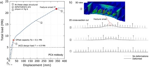
The simulation results are presented and compared against design loads in Table 12. The ratio of plastic capacity to design load (F_p/F) can be treated as an overload factor in relation to the design load. For all designs, this factor remains in the range of 1.4–2.1, suggesting that the presented approach generates designs with a relatively high safety margin against plastic collapse. This indicates that the approach is suitable for the preliminary design stage for the determination of reasonable albeit conservative scantlings that can be further optimized in later design stages.

Table 12. Simulation results compared against design load.

	PC3			PC4			PC5			PC6			PC7
	Bow	Mid	Stern	Bow	Mid	Stern	Bow	Mid	Stern	Bow	Mid	Stern	Bow	Mid	Stern
Design load F (MN)	15.1	6.6	7.8	10.5	4.9	5.4	7.3	3.1	3.1	7.6	2.1	1.9	5.8	1.6	1.3
Plastic capacity Fp (MN)	25	10.4	11.2	20	8.1	9.05	13.5	5.55	4.56	13.33	3.9	3.9	10.81	2.6	2.4
Fp/F (-)	1.7	1.6	1.4	1.9	1.6	1.7	1.9	1.8	1.5	1.8	1.8	2.1	1.9	1.6	1.9
Fracture load Ff (MN)	55	30.5	29.1	43	21.7	23.8	35.3	15.7	16.5	38.1	13.2	12.9	32	12.3	11.9
Ff/F (-)	3.6	4.6	3.7	4.1	4.4	4.4	4.9	5.1	5.4	5.0	6.2	6.8	5.6	7.6	9.5

While the applied approach using a rule-based uniform pressure on a fixed patch might be sufficient for the determination of plastic capacity, the application of the approach should not be extrapolated to highly complex processes such as that of ice-structure interaction (see discussion in section 4). Accordingly, the load-displacement curves beyond the point of plastic capacity in Figure 14 are presented for illustrative purposes only. Because in each analysis the fracture onset occurred in the framing members, the structure appears to remain watertight at this point. Table 12 shows that the ratio of fracture load to design load (F_f/F) increases with ice class. Compared to plastic capacity, this ratio has a wider scatter ranging from 3.6–9.5. The wider scatter can be explained by the complex nature of the structural collapse and differences in load shedding mechanisms between structures. These differences between collapse mechanisms also explain why lower ice class vessels tend to yield higher safety factors against structural fractures; slender and less rigid structures are more effective in distributing loads evenly across the structure to neighbouring frames, delaying the fracture onset. Considering the significant scatter in the obtained F_f/F-ratios, the use of direct analysis methods and more refined analysis methods are recommended when analysing a ship’s safety against fracture.

Figure 14. A conceptual framework for life-safety consequence severity for Arctic ship evacuations (Browne et al. 2021).

A strength of the above presented approach for the dimensioning of the primary structural members of Polar Class hull structures is that it is based on closed-form expressions, which makes it straightforward to apply and to integrate into established design processes. Finite element-based analyses indicate that the approach generates designs with a relatively high safety margin against plastic collapse. Thus, the proposed approach appears well-suited for the preliminary design stage for the determination of reasonable albeit conservative scantlings that can be further optimized in later design stages. It is noted that the above analyses were carried out using idealized ice loads. Future studies using more detailed ice load models are recommended for improved understanding of the actual safety margins of Polar Class hull structures.

6. Accident consequence modelling

6.1. Life-safety consequences

The life-safety category of a ship reflects the potential consequences to crew and passenger safety resulting from an evacuation in Arctic waters. A scenario-based life-safety consequence model for Arctic ship evacuations was developed by Browne et al. (2021). The consequence model includes a qualitative conceptual framework and quantified consequence severities for different Arctic ship evacuation scenarios. The conceptual framework was developed based on expert knowledge elicited through semi-structured interviews. Scenario-based consequence severities were established based on expert evaluations elicited through a rating survey. Main results relevant to the proposed Arctic shipping operational risk management framework presented in chapter 3 are outlined in the following.

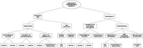
The conceptual framework for life-safety consequence severity for Arctic ship evacuations is presented in Figure 14. The crux of any successful ship evacuation is the ability of evacuees to survive until rescue. Response time and survivability are the primary factors identified by interview participants as influencing consequence severity and thus represent the two main branches of the conceptual framework.

A number of influencing factors define response time and survivability. At the most granular level, there are six common influencing factors: season, region, governance and regulation, ship type, risk tolerance of the ship operator, and accident type.

Life-safety risk is an area of risk concerning the level of harm to humans, considering ill-health, injury, and death. A five-point severity index is used to model life-safety consequences, corresponding to orders of magnitudes of equivalent fatalities (Table 13). Severity levels range from minor to disastrous and equivalent fatality values are defined for each. Life-safety consequence severity was evaluated for Arctic ship evacuation scenarios. Factors and associated levels used to define the scenarios are presented in Table 14. Five ship types with associated POB numbers were evaluated for each scenario as per Table 15.

Table 13. Life-safety consequence severity definitions, modified from the FSA guidelines (IMO 2018).

Severity index	Severity	Effects on human safety	Equivalent fatalities
1	Minor	Single or minor injuries	0.01
2	Severe	Multiple or severe injuries	0.1
3	Significant	Single fatality or multiple severe injuries	1
4	Catastrophic	Multiple fatalities	10
5	Disastrous	Large number of fatalities	100

Table 14. Factors used to define evacuation scenarios (Browne et al. 2021).

Factors	Levels
Season	Summer	Winter
Ice conditions	Sea ice	Open water
Wind/sea state	Calm	Severe
Evacuation	Controlled	Uncontrolled
Response time	12 hrs 24 hrs	2 days 5 days

Table 15. Ship types and POB numbers evaluated for evacuation scenarios (Browne et al. 2021).

Ship type	POB
Passenger vessel (e.g. expedition cruise ship)	250
Passenger vessel (e.g. standard cruise ship)	1,000
Cargo vessel	25
Fishing vessel	10
Pleasure craft	10

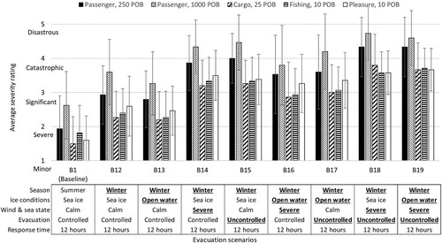
Average severity ratings for the nineteen evacuation scenarios are plotted below. The factors used to define each scenario are presented in the boxes directly below the axis. For clarity, scenario factors that are different from the baseline are underlined and bold. Standard deviation bars are plotted for each scenario.

The effect of response time on life-safety consequence severity is presented in Figure 15. Summer evacuation scenarios are presented in Figure 16. Winter evacuation scenarios are presented in Figure 17.

Figure 15. The effect of response time on the average life-safety consequence severity (Browne et al. 2021).

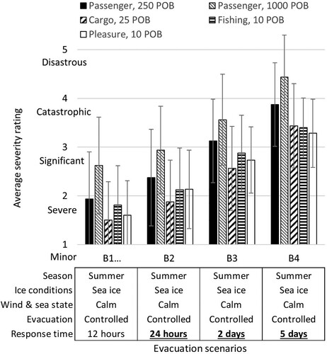
Figure 16. Average life-safety consequence severity, summer scenarios (Browne et al. 2021).

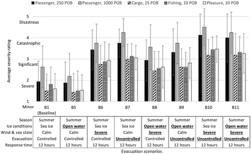
Figure 17. Average life-safety consequence severity, winter scenarios (Browne et al. 2021).

Ship type has a significant influence on consequence severity following evacuation in Arctic waters. Results show evacuation of high POB passenger vessels poses the highest consequence severity of evaluated ship types.

Response time was evaluated as having the greatest level of influence on the expected number of fatalities. Severity level increases dramatically with response time. Even under optimal conditions (i.e. summer, calm weather, controlled evacuation), a response time of five days is expected to result in multiple fatalities for all assessed ship types.

The time available to evacuate is a sub-theme under survivability, influencing the level of preparedness of those on board for evacuation and survival. It was rated to have the second greatest level of influence on the expected number of fatalities. Aside from response time, an uncontrolled evacuation, such as a rapid capsize, is the most significant contributor to increased consequence severity.

6.2. Ecological consequences

The most significant environmental risk of Arctic shipping is that of an oil spill. This is because oil spills can have devastating and long-lasting consequences to the coastal and marine ecosystems as in cold and icy conditions, oil weathering processes are reduced and slowed down (Afenyo et al. 2016). As a result, the decomposition of oil is prolonged, and the recovery of the environment slow (Brandvik et al. 2006; AMAP 2010; Fingas and Hollebone 2013). As per the current regulations, to protect the environment, ships operating in polar regions must be MARPOL compliant, e.g. in terms of structural arrangements and the location of fuel oil tanks. In addition, for vessels of Category A and B, the Polar Code specifies additional requirements for the location of tanks carrying noxious liquid substances.

Several methods exist to assess the ecological impacts of an oil spill. The trajectory and fate of spilled oil can be modelled with advanced mechanistic spill trajectory simulators, see e.g. SIMAP (2021), French McCay (2004), and Wilson et al. (2018). However, the application of such sophisticated models is not straightforward as they must first be calibrated to the local environmental conditions of the considered spill location, which requires extensive data on bathymetry, weather, and habitat types, among others. Because the required data is not available for most Arctic regions, the application of trajectory models remains limited to specific spill locations (Nordam et al. 2017; Wilson et al. 2018). Another limitation of such models relates to their ability to handle uncertainties.

From a holistic uncertainty treatment point of view, the most common approaches for assessing ecological consequences of oil spills are based on Bayesian Networks (BNs), See for instance Sajid et al. (2020) and Fahd et al. (2021). BNs provide a convenient way to model a system and to express uncertainties explicitly, but they appear mainly suited to model specific scenarios at fixed locations, and they lack the mechanistic process understanding present in oil trajectory models. Moreover, oil spill trajectory and BN models have not been generalized for large areas (e.g. an entire shipping route).

6.2.1. Probabilistic method to assess ecological impacts of oil spills

Considering the above, we recommend considering a holistic probabilistic approach for assessing the impacts of oil spills on Arctic marine ecosystems by Helle et al. (2020). Their model applies a Bayesian perspective, which is well justified for Arctic risk management both because it enables measuring uncertainty in terms of probability, and because it allows a coherent integration of different knowledge sources ranging from expert opinions to statistical models to mechanistic simulators (Nevalainen et al. 2017; Helle et al. 2020). As a result, the method can cope with the typically limited amount of data available and take into account modelling uncertainties in a holistic and explicit manner. This is important as the modelling uncertainties typically are significant (Emmerson and Lahn 2012). Also, the method allows assessing the ecological impacts of oil spills over large areas and different seasons. The model, an overview of which is presented in Figure 18, includes the following:

• Seasonally and spatially varying species-specific population distributions, see e.g. Mäkinen and Vanhatalo (2018).

• Seasonally and spatially varying spreading of oil, which together, determine the proportion of the population of a given species that is present in the oiled area.

• Seasonally and spatially varying accident probability, see Vanhatalo et al. (2021).

• Seasonally varying, species-specific exposure potentials (i.e. the probability that an individual is exposed to oil if present in the oiled area) and sensitivities (the probability that exposed individual dies due to the oil exposure), see Nevalainen et al. (2018).

Figure 18. Overview of the probabilistic oil spill risk assessment method by Helle et al. (2020). Reproduced with permission.

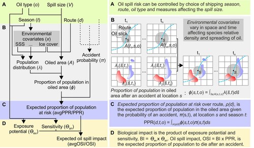
As per Figure 18, the model considers a set of relevant factors as well as their conditional interdependencies. Each factor is a random variable, the probability distribution of which depends only on the state of the factors preceding it (arrows). The dashed arrows leading to ‘Accident probability’ illustrate that the probability of an accident may be affected by several factors, see for instance Vanhatalo et al. (2021), although these were not explicitly modelled by Helle et al. (2020). Nevertheless, the model (see Figure 18) considers different categories of factors affecting the proportion of the population that will perish including the following:

1. Factors that can be controlled by management decisions.

2. Seasonally and spatially varying factors. Red and purple areas as shown in Figure 18 represent the population distributions of two species. Environmental covariates and population distribution are stochastic spatiotemporal functions represented as random raster maps (with 5 × 5 km grid cells) that account for environmental stochasticity and parameter uncertainty in species distribution models. The oiled area and the proportion of a population in an oiled area are stochastic spatiotemporal functions represented as random vectors over route points.

3. The expected proportion of a population at risk, i.e. the proportion of a population present in the oiled area.

4. Seasonally varying species-specific exposure potential and sensitivity and seasonally varying route-specific oil spill impact, i.e. the proportion of the population that perish due to oiling. (Risk measures: _avgPPR = expected proportion of a population present in the oiled area; PPR = route-specific risk scaled by the route length; _avgOSI = the expected oil spill impact, defined as _avgOSI = _avgPPR × BI; OSI = the route-specific risk scaled by the route length; BI = biological impact, defined as BI = exposure potential × sensitivity).

As indicated above, using the model, it is possible to estimate the proportion of a species population that dies acutely (e.g. within two weeks) following an oil spill. Because the uncertainty related to each factor contributing to the ecological impact is expressed in terms of a probability distribution, the results express uncertainty explicitly as well.

Helle et al. (2020) demonstrate the utility of the method in a case study dealing with an oil spill in the Kara Sea. Specifically, they assessed the ecological impacts of oil spills on three Arctic marine mammal (AMM) species: polar bear (Ursus maritimus), ringed seal (Pusa hispida), and walrus (Odobenus rosmarus). The assessment considered four types of oil, three seasons, and five shipping routes. The results indicate that the acute impacts differ between species, shipping routes, oil types, and seasons. Although heavier oils are more detrimental to AMMs than lighter oils, see Nevalainen et al. (2018), the latter spread more efficiently than heavier oils both in open water and in ice, exposing greater proportions of AMM populations to oil. This highlights the importance of spatially explicit and season-specific ecological impact assessments in the Arctic. Because several of the physical factors influencing the Arctic biota, such as sea ice, vary both seasonally and interannually, see Kovacs et al. (2011), and because population densities hence also vary, it is not advisable to base impact assessments on areal species densities averaged over seasons, as this might lead to erroneous conclusions.

Limitations of the method by Helle et al. (2020) that should be addressed in future research include the following. First, the method applies a somewhat oversimplified approach to describe the spreading of oil, which does not consider oil weathering or the transport of oil by currents, winds, and ice. Hence, the development of a more realistic, but at the same time computationally feasible, spill trajectory model is motivated. Second, while the method focuses on the acute ecological impacts of an oil spill, it does not consider the associated long-term effects. The consideration of long-term effects should be included into assessment because, e.g. species differ in their ability to recover from population declines, which can be more detrimental for species that mature late and have few offspring than for species that mature early and breed annually. Also, some species are sensitive to long-term impacts of oiling, and oil spills can also affect species indirectly via long-term changes in food webs (Chapman and Riddle 2005). Third, it is evident that any comprehensive risk assessment should include a variety of ecological components representing different trophic levels and functional groups.

6.2.2. Sensitivity as a proxy for ecological consequences

As an alternative to impact analysis, some environmental risk assessment approaches do not consider the ecological consequences per se, but rather analyse the sensitivity of an ecosystem to oil, e.g. in terms of the likelihood that an individual will suffer adverse effects (including death) if oiled. In this perspective, all biotas are sensitive to oil, but their level of sensitivity depends on their physiological characteristics. For instance, seabirds are sensitive to oil, as their thermoregulation is based on the insulation capacity of their feathers: if a bird’s feathers become oiled, the insulation is lost, and the bird will likely die of hypothermia. By contrast, for marine mammals with subcutaneous blubber (a type of skin), oiling may not be very detrimental as their thermoregulation is not dependent on fur. However, they might instead suffer from the toxicological effects of oil if, for instance, they ingest oily prey (Wallace et al. 2017; Nevalainen et al. 2019). In addition, the sensitivity to oil may vary between different life-stages, e.g. fish eggs and fry are typically considerably more sensitive to oil than adults. There also are differences in sensitivity between different habitats. The well-established Environmental Sensitivity Index (ESI) classifies shoreline types by their properties, including their exposure to wave and tidal energy and the general biological productivity and sensitivity (Gundlach and Hayes 1978). Following this system, exposed rocky shores are classified as the least sensitive, whereas marshes, swamps, and mangroves are classified as the most sensitive shoreline types.

Studies on the ecological or environmental sensitivity to oil consider other ecological attributes as well, such as threatened species and habitats and protected areas. A threatened species is one that is facing a high risk of extinction in the wild (IUCN 2021). Even if such species were not highly sensitive to oil per se, if already imperilled, they may nevertheless be severely affected by an oil spill. Correspondingly, specific areas are protected because of their recognized ecological or other values. In many countries, both threatened species and protected areas are protected by law.

There are many different approaches to identify and quantify the sensitivity of marine and coastal areas to oil spills, including those by Fattal et al. (2010) and Santos et al. (2013). However, only a few of them have been applied to the Arctic. A comprehensive approach covering the whole Arctic is presented by AMAP/CAFF/SDWG (2013), which provides means for the identification of important areas but not for the scoring of the sensitivity of different areas. An approach for the scoring of the ecological sensitivity of Arctic areas is provided by the ‘Guideline for Arctic Marine Risk Assessment’, see EPPR (2021). Common elements of approaches for the classification and rating of ecological sensitivity include: (a) consideration of protected and other important areas, (b) consideration of threatened or endangered species, and (c) consideration of other species and habitats sensitive to oil.

6.2.3. Concluding remarks

Regarding the best practices for assessing ecological consequences of shipping-induced oil spills in the Arctic, the following is recommended:

• As the Arctic environment is characterized by high temporal and spatial variation, assessments must be conducted season-wise and with a high spatial resolution to cover the dynamic nature of the Arctic environment. Spatial variation is important to consider also for instance when comparing different routes and their level of risk.

• Because shipping routes can be hundreds of nautical miles in length, it is not sufficient to assess the ecological impacts of potential spills only for a few selected locations as the entire route should be considered.

• All types of oil spills are detrimental to the environment, but the harmfulness of different oil types is different for different species. Hence, the assessments must cover different oil types and a variety of species and groups of species living in different habitats (e.g. seafloor, water column, shoreline, ice, polynyas, etc.).

• As uncertainty typically has a major role in decision-making and risk management, it is important to develop assessment methods that consider uncertainty explicitly. Uncertainty due to a lack of knowledge can be reduced through further research and data gathering, whereas uncertainty due to natural variability cannot. Understanding the nature of uncertainty may enable an efficient allocation of resources to reduce uncertainty.

• Insufficient data is a general challenge when dealing with issues concerning the Arctic environment. To make the most use of the available data, probabilistic (Bayesian) methods should be applied. If the availability of data is limited, it should be supplemented by expert opinion obtained through a carefully planned, executed and documented elicitation process. In many Arctic regions, the monitoring of the biota is still relatively poor and sporadic. To be able to assess the ecological consequences of oil spills realistically, systematic surveys to collect accurate data on species ranges and abundances should be established.

• When ecological sensitivity is mapped, very large areas may be classified as sensitive. Although most Arctic areas can be considered sensitive, practically uniform sensitivity classifications do not support decision-making as it does not enable differentiation between areas. Hence, relevant scoring schemes should be applied. In addition, as species’ ranges can cover very large areas, core areas of different species must be identified. Otherwise, sensitivity maps and related risk assessments may fail to identify the most critical areas.

6.3. Socio-economic consequences

Shipping accidents resulting in oil spills may have dramatic socio-economic impacts at both local and regional levels as an oil spill typically harm multiple economic sectors simultaneously, including fisheries, aquaculture, tourism, port businesses, and water intake activities. In addition, oil spills can cause severe social impacts on local communities, including stress and social breakdown (Chang et al. 2014). The situation is alarming in the Arctic where the way of life and traditional livelihoods of indigenous people are tightly linked to the Arctic environment.

Assessing the socio-economic impacts generally includes defining, categorizing, and quantifying relevant indicators. However, the socio-economic impacts of oil spills can be defined in various ways, because as per Olsen et al. (2019), the impact of an oil spill depends on the local context as well as on the perceptions and use of the natural environment. Therefore, selecting and quantifying the most relevant or the most suitable socio-economic indicators is challenging.

The socio-economic consequences of an oil spill can be categorized for instance as per the methodology of Transport Canada for risk assessment in Canadian waters, see Dillon Consulting (2017). The methodology divides socio-economic components into seven subcategories: commercial fishing, tourism employment, freight tonnage, water resources extraction, First Nations, population density, and parks and cultural areas. The indicators are quantified using various methods. Commercial fishing intensity can be assessed in various ways, e.g. by the total catch or by its monetary value. As the characteristics of commercial fishing and the available data vary between regions, the user can choose the most appropriate method considering the available data (Dillon Consulting 2017). Some other indicators, e.g. those concerning First Nations as well as Parks and cultural areas, are based mainly on their presence in the area. However, the indicators presented above and the way they are quantified may not apply to the whole Arctic, as commercial fishing, for instance, occurs only in some Arctic regions.

Considering the above, to be able to assess the potential socio-economic consequences of an oil spill in the Arctic, it is important to notice that it may not be feasible to apply the same methods as used for non-Arctic areas. This is because assessing the consequences of an oil spill in the Arctic requires the consideration of unique local factors. Examples of such local factors are presented by the Nunavut Planning Commission (2013).

Some research also exists on monetizing the effects of oil spills in the Arctic (Afenyo et al. 2019, 2021). Specifically, Afenyo et al. (2019) provide a method for assessing the impacts of oil spills in monetary terms using Bayesian networks (BNs) to collectively estimate the related social, economic, and biophysical impacts. While the study by Afenyo et al. (2019) provides a tool for assessing impacts in a global context, Afenyo et al. (2021) focus on the Canadian Arctic and utilizes influence diagrams (IDs) to assess socioeconomic risks in monetary terms.

To summarize, further research is needed to improve the understanding of the local consequences of oil spills in the Arctic. There is also a need to develop methods to include indigenous and other local knowledge in identifying ecologically or socio-economically significant areas. Potential methods for this include participatory mapping and community-based research (Dawson, et al., 2020a, 2020b), participatory scenario methodologies (Nilsson et al. 2019), and decision support tools (DSTs) such as the existing Nunaliit Atlas Framework or the Inuit Siku (sea ice) Atlas, both presented by Carleton University (2021a, 2021b). Further, the Pikialasorsuaq (North Water Polynya) Region Atlas (WWF, KNAPK, ICC Greenland, ICC Canada, Dalhousie University 2021) is a digital atlas tool that displays information on the ecological and cultural importance of different areas. The atlas also provides an ArcGIS-based tool to help with future planning of shipping in the North Water Polynya.

7. Conclusions

Risk management in Arctic shipping requires anticipating the ice conditions that a ship is expected to encounter. For this purpose, ice charts are an important source of data. Most ice charts covering the Arctic describe ice conditions following the international so-called egg code standard. A general limitation of such ice charts is that their ice thickness estimates are subject to significant uncertainty, and that they provide no or limited information on important factors such as ice ridging, pressured ice, and ice strength. Considering these limitations, a more precise standard would be welcome. Meanwhile, to compensate for the limitations, the available ice chart data can be supplemented with data obtained through in-situ measurements and observations.

For the purpose of assessing ship operations in ice, egg code data may be converted into an equivalent ice thickness value. However, there is no generally accepted definition of equivalent ice thickness, but several competing ones. It should also be noted that the concept of equivalent ice thickness, which effectively averages out local sea ice variations, may not be appropriate for all types of assessments.

Vessels operating in the Arctic are subject to the Polar Code. Under this code, ship operators are required to undertake an operational assessment to establish vessel-specific operational limitations with regards to operation in ice, among others. For this purpose, the Polar Code recommends the use of the POLARIS methodology. POLARIS assesses the risk of a ship being damaged by ice considering the ice conditions and the ship’s assigned Polar Class notation. While POLARIS has been shown to well reflect the structural risk for typical ships and operations, the current methodology does not account for the potential consequences of ice-induced ship damage. To address this limitation, an extended version of POLARIS is proposed that considers the magnitude of potential consequences. Following the proposed approach, vessels with higher potential consequences (e.g. life-safety, environmental, or socio-economic) should be operated more conservatively.

While POLARIS can roughly assess the risk of a ship suffering structural damage due to ice loading, users need to be aware that the method quantifies risk in terms of a non-dimensional risk index. To assess the actual safety of a ship with regards to ice loading, its expected ice loads must be calculated. Available methods for this purpose can be divided into three main categories: (a) theoretical or first-principle, (b) semi-empirical, and (c) empirical. Different methods are suitable for different purposes. Nevertheless, regardless of category, presently all methods have significant limitations, most of which relates to a general lack of relevant input and validation data. This is due to significant challenges related to full-scale ice load measurements, especially in terms of linking of ice loads and ice conditions. To address this issue, methods are being developed to support systematic and automatic monitoring of a ship’s ice exposure. It is noted that the development of new and improved ice load assessment approaches is well motivated as these may provide a path towards goal-based structural design and regulatory approval, potentially resulting in improved safety and efficiency.

Under the Polar Code, the hull structural design of ships intended for operations in ice must be carried out in accordance with an appropriate Polar Class or equivalent standard. The Polar Class rules determine the minimum required scantlings of local structural members by a set of closed form equations. For large primary structural members (e.g. transverse web frames), on the other hand, only strength criteria are determined, the fulfilment of which must be demonstrated using direct structural analysis methods. Because the related calculations are laborious, to support designers at the conceptual design phase, an approach based on closed-form expressions that define reasonable scantlings for primary structural members is proposed.

A maritime accident in the Arctic may have a range of consequences, including loss of life, injury, environmental damage, and economic (including socio-economic) losses. For the assessment of life-safety consequences associated with a ship evacuation in Arctic waters, a five-point severity index is proposed that corresponds to orders of magnitudes of equivalent fatalities. Evacuation scenarios consider different ship types and numbers of personnel on board, estimated response time, season, ice and metocean conditions, and the time available for evacuation. The most significant environmental risk of Arctic shipping is that of an oil spill. For the assessment of the environmental consequences of an oil spill, a probabilistic method is proposed. The proposed model considers a range of probabilistic factors, including (a) seasonally and spatially varying species-specific population distributions, (b) seasonally and spatially varying oil spreading patterns, (c) seasonally varying and species-specific exposure coefficients defining the probability that an individual is exposed to oil if present in an oiled area, and (d) estimates of the probability that exposed individuals perish due to oil exposure. As the Arctic environment is characterized by high temporal and spatial variation, assessments must be conducted season-wise and with a high spatial resolution to cover the dynamic nature of the Arctic environment. When assessing the potential economic and socioeconomic consequences of an oil spill, it is necessary to consider that the impact of a spill may be dramatic at local and regional levels, as it may simultaneously cause harm to multiple economic sectors, including fisheries, aquaculture, tourism, port businesses, and water intake activities. Other potential types of social impacts on local communities include stress and social breakdown, especially in the Arctic where the way of life and traditional livelihoods of indigenous people are tightly linked to the Arctic environment.

Disclosure statement

No potential conflict of interest was reported by the author(s).

Correction Statement

This article has been republished with minor changes. These changes do not impact the academic content of the article.

Additional information

Funding

This work was supported by the Lloyd's Register Foundation (100077), a charitable foundation, helping to protect life and property by supporting engineering-related education, public engagement and the application of research www.lrfoundation.org.uk.

References

- AARI. 2021a. Website of the Arctic and Antarctic Research Institute. [accessed 2021 Jul 5]. http://www.aari.ru/main.php?lg=1&id=54.
- AARI. 2021b. Website of AARI. Reference tables for International and Russian national symbology. [accessed 2021 Jul 5]. http://www.aari.ru/gdsidb/docs/wmo/code_tables_en.pdf.
- Abramov V. 1996. Atlas of Arctic icebergs: the Greenland, Barents, Kara, Laptev, East-Siberian and Chukchi Seas and the Arctic Basin. Paramus: Backbone Publishing Company.
- Afenyo M, Jiang C, Ng AKY. 2019. Climate change and Arctic shipping: a method for assessing the impacts of oil spills in the Arctic. Transp Res D. 77:476–490.
- Afenyo M, Ng AKY, Jiang C. 2021. A multiperiod model for assessing the socioeconomic impacts of oil spills during Arctic shipping. Risk Anal. https://doi.org/10.1111/risa.13773.
- Afenyo M, Veitch B, Khan F. 2016. A state-of-the-art review of fate and transport of oil spills in open and ice-covered water. Ocean Eng. 119:233–248.
- AMAP. 2010. Assessment 2007: oil and gas activities in the Arctic – effects and potential effects. Vol. I. Oslo: Arctic Monitoring and Assessment Programme (AMAP).
- AMAP/CAFF/SDWG. 2013. Identification of Arctic marine areas of heightened ecological and cultural significance: Arctic Marine Shipping Assessment (AMSA) IIc. Oslo: AMSA.
- Ashton GD. 1986. River lake Ice engineering. 1st ed. Highlands Ranch: Water Resources Publications LLC.
- Benz L, Münch C, Hartmann E. 2021. Development of a search and rescue framework for maritime freight shipping in the Arctic. Trans Res Part A. 152:54–69.
- Bergström M, Leira BJ, Kujala P. 2020. Future scenarios for Arctic shipping. ASME 2020 39th International Conference on Ocean, Offshore and Arctic Engineering (OMAE 2020).
- Bergström M, Li F, Suominen M, Kujala P. 2022. A goal-based approach for selecting a ship’s polar class. Mar Struct. 81:103123.
- Billard R, Rahman MS, Kennedy A, Simões Ré AJ, Veitch B. 2014. Operability of lifeboats in pack ice: coxswains’ skill and design factors. Offshore Technology Conference; Houston, Texas.
- Brandvik P, Sorheim K, Singsaas I, Reed M. 2006. Short state-of-the-art report on oil spills in ice-infested waters. Oil behaviour and response options. SINTEF Materials and Chemistry. Report No. STF80MKA06148. Trondheim: SINTEF.
- Browne T, Taylor R, Jordaan I, Gürtner A. 2013. Small-scale ice indentation tests with variable structural compliance. Cold Reg Sci Technol. 88:2–9.
- Browne T, Taylor R, Veitch B, Kujala P, Khan F, Smith D. 2020. A framework for integrating life-safety and environmental consequences into conventional Arctic shipping risk models. Appl Sci. 10(8):2937.
- Browne T, Veitch B, Taylor R, Smith J, Smith D, Khan F. 2021. Consequence modelling for Arctic ship evacuations using expert knowledge. Mar Policy. 130:104582.
- Canadian Ice Service. 2021a. Daily Iceberg analysis chart Newfoundland and Labrador Coasts. [accessed 2021 Jul 8]. https://ice-glaces.ec.gc.ca/cgi-bin/getprod.pl?prodid=WIS65&wrap=1&lang=en&q=2.
- Canadian Ice Service. 2021b. Ice forecasts and observations. [accessed 2021 Jun 15]. https://www.canada.ca/en/environment-climate-change/services/ice-forecasts-observations.html.
- Carleton University. 2021a. The Nunaliit Atlas Framework. [accessed 2021 Jul 8]. http://nunaliit.org/.
- Carleton University. 2021b. Inuit Siku Atlas. [accessed 2021 Dec 20]. https://sikuatlas.ca/index.html.
- Chai W, Leira BJ, Høyland KV, Sinsabvarodom C, Yu Z. 2021. Statistics of thickness and strength of first-year ice along the Northern Sea route. J Mar Sci Technol. 26:331–343.
- Chang S, Stone J, Demes K, Piscitelli M. 2014. Consequences of oil spills: a review and framework for informing planning. Ecol Soc. 19(2):26.
- Chapman P, Riddle M. 2005. Toxic effects of contaminants in polar marine environments. Environ Sci Technol. 39(9):200A–206A.
- Cundall PA, Strack O. 1979. A discrete numerical model for granular assemblies. Géotechnique. 29(1):47–65.
- Daley C, Daley K, Dolny J, Quinton B. 2017. Overload response of flatbar frames to ice loads. Ships Offsh Struct. 12(Issue sup1):S68–S81.
- Daley C, Kendrick A, Appollonov E. 2001. Plating and framing design in the unified requirements for polar class ships. Proceedings of the 16th International Conference on Port and Ocean Engineering Under Arctic Conditions (POAC); Ottawa, Ontario, Canada.
- Daley CG. 1999. Energy based ice collision forces. Proceedings of the 25th International Conference on Port and Ocean Engineering under Arctic Conditions (POAC); Helsinki.
- Daley CG. 2002. Derivation of plastic framing requirements for polar ships. Mar Struct. 15(6):543–559.
- Daley CG, Ferregut C, Brown R. 1991. Structural risk model of Arctic shipping. In: Jones S, Tillotson J, McKenna RF, Jordaan IJ editors. Ice-structure interaction. International union of theoretical and applied mechanics (International Association for Hydraulic Research). Berlin: Springer; p. 507–540.
- Dawson J, Carter N, van Luijk N, Parker C, Weber M, Cook A, Grey K, Provencher J. 2020a. Infusing inuit and local knowledge into the low impact shipping corridors: an adaptation to increased shipping activity and climate change in Arctic Canada. Environ Sci Policy. 105:19–36.
- Dawson J, Carter NA, van Luijk N, Weber M, Cook A. 2020b. Arctic corridors and northern voices project: methods for community-based participatory mapping for low impact shipping corridors in Arctic Canada. MethodsX. 7:101064.
- Dillon Consulting. 2017. Area risk assessment methodology development for ship-source oil spills in Canadian waters – Guidance Document 15-1623. Ottawa: Transport Canada.
- DMI. 2022. Webpage of the Danish Meteorological Institute. Ice charts around Greenland. [accessed 2022 Jan 15]. http://ocean.dmi.dk/arctic/icecharts.uk.php.
- Dumanskaya IO. 2014. Ice conditions of the seas of the European part of Russia. Moscow: IG-SOTSIN.
- Emmerson C, Lahn G. 2012. Arctic opening: opportunity and risk in the high north project report. London: Lloyd’s and Chatham House.
- EPPR. 2021. Guideline for Arctic marine risk assessment. [accessed 2021 Jun 7]. https://eppr.dnvgl.com/.
- Erceg B, Taylor R, Ehlers S, Leira BJ. 2014. A response comparsion of a stiffened panel subjected to rule-based and measured ice loads. Proceedings of ASME 2014 33rd International Conference on Ocean, Offshore and Arctic Engineering.
- Fahd F, Yang M, Khan F, Veitch B. 2021. A food chain-based ecological risk assessment model for oil spills in the Arctic environment. Mar Pollut Bull. 166:112164.
- Fattal P, Maanan M, Tillier I, Rollo N, Robin M, Pottier P. 2010. Coastal vulnerability to oil spill pollution: the case of Noirmoutier Island (France). J Coast Res. 265:879–887.
- Fedi L, Etienne L, Faury O, Rigot-Müller P, Stephenson S, Cheaitou A. 2018. Arctic navigation: stakes, benefits and limits of the POLARIS system. J Ocean Technol. 13(4):60–71.
- Fingas M, Hollebone B. 2013. Oil behaviour in ice-infested waters, The Arctic Marine Oilspill Program (AMOP). Halifax; p. 110–135.
- French McCay D. 2004. Oil spill impact modeling: development and validation. Environ Toxicol Chem. 23(10):2441–2456.
- Gagnon R. 2011. A numerical model of ice crushing using a foam analogue. Cold Reg Sci Technol. 65(3):335–350.
- Gagnon R, Andrade SL, Quinton B, Daley C, Colbourne B. 2020. Pressure distribution data from large double-pendulum ice impact tests. Cold Reg Sci Technol. 175:103033.
- Gong H, Polojärvi A, Tuhkuri J. 2019. Discrete element simulation of the resistance of a ship in unconsolidated ridges. Cold Reg Sci Technol. 167:102855.
- Gundlach E, Hayes M. 1978. Vulnerability of coastal environments to oil spill impacts. Mar Technol Soc J. 12:18–27.
- Helle I, Mäkinen J, Nevalainen M, Afenyo M, Vanhatalo J. 2020. Impacts of oil spills on Arctic marine ecosystems: a quantitative and probabilistic risk assessment perspective. Environ Sci Technol. 54(4):2112–2121.
- Herrnring H, Ehlers S. 2021. A finite element model for compressive ice loads based on a Mohr-Coulomb material and the node splitting technique. J Offshore Mech Arct Eng. 144(2):021601.
- Herrnring H, Kubiczek JM, Ehlers S. 2020. The ice extrusion test: a novel test setup for the investigation of ice-structure interaction – results and validation. Ships Offsh Struct. 15(sup1):S1–S9.
- Hopkins M. 1992. Numerical simulation of systems of multitudinous polygonal blocks. Tech. Rep. 92-22. Hanover, New Hampshire: Cold Regions Research and Engineering Laboratory, CRREL.
- IACS. 2016. Requirements concerning polar class. London: International Association of Classification Societies.
- Idrissova S, Bergström M, Hirdaris SE, Kujala P. 2019. Analysis of a collision-energy-based method for the prediction of Ice loading on ships. Appl Sci. 9(21):4546.
- IMO. 2015. International code for ships operating in polar waters (Polar Code). MEPC 68/21/Add.1 Annex 10. London: International Maritime Organization.
- IMO. 2016. Guidance on methodologies for assessing operational capabilities and limitations in ice. MSC.1/Circ.1519. London: International Maritime Organization.
- IMO. 2018. Revised guidelines for formal safety assessment (FSA) for use in the IMO rule-making process. MSC-MEPC.2/Circ.12/Rev.2. London: International Maritime Organization.
- IMO. 2019. Generic guidelines for developing IMO goal-based standards. MSC.1/Circ.1394/Rev.2. London: International Maritime Organization.
- ISO. 2010. ISO 19906:2010. Petroleum and natural gas industries—Arctic offshore structures. Geneva: International Standard Organization (ISO).
- IUCN. 2021. The IUCN Red list of threatened species. Version 2021-1. [accessed 2021 Jun 7]. https://www.iucnredlist.org.
- Jordaan I, Maes M, Brown P, Herman I. 1993. Probabilistic analysis of local ice pressure. Offshore Mech Arct Eng. 115:83–89.
- Jordaan IJ. 1987. Probabilistic analysis of environmental data for design of fixed and mobile Arctic offshore structures. Proceedings of the Fifth International Conference on Applications of Statistics and Probability in Soil and Structural Engineering (ICASP). Vancouver.
- Jordaan IJ. 2001. Mechanics of ice–structure interaction. Eng Fract Mech. 68(17-18):1923–1960.
- Kämäräinen J, Riska K. 2017. Ice class rules and international regulations. In: Carlton J, Jukes P, Choo YS, editors. Encyclopedia of Maritime and offshore engineering. Hoboken (NJ): John Wiley & Sons, Ltd; p. 1–13.
- Kellner L, Lu W, Ehlers S, Høyland KV. 2021. Study on the cohesive edge crack in a square plate with the cohesive element method. Int J Fract. 231:21–41.
- Kendrick A, Daley C. 2011. Structural challenges faced by Arctic ships. SSC-461. Washington (DC): Ship Structure Committee.
- Khan B, Khan F, Veitch B. 2020. A dynamic Bayesian network model for ship-ice collision risk in the Arctic waters. Saf Sci. 130:104858.
- Kim H, Daley C, Colbourne B. 2015. A numerical model for ice crushing on concave surfaces. Ocean Eng. 106:289–297.
- Kolari K, Kurkela J. 2012. Ship-ice collision analysis. VTT-R-07666-12, Espoo: VTT.
- Kõrgesaar M, Kujala P, Romanoff J. 2018. Load carrying capacity of ice-strengthened frames under idealized ice load and boundary conditions. Mar Struct. 58:18–30.
- Kotilainen M, Suominen M, Kujala P. 2019. Rotating ice cusps on ship's bow shoulder: full-scale study on the cusp sizes and corresponding peak loads in different ice and operational conditions. Ocean Eng. 189(1):106280.
- Kotilainen M, Vanhatalo J, Suominen M, Kujala P. 2017. Predicting ice-induced load amplitudes on ship bow conditional on ice thickness and ship speed in the Baltic Sea. Cold Reg Sci Technol. 135:116–126.
- Kotilainen M, Vanhatalo J, Suominen M, Kujala P. 2018. Predicting local ice loads on ship bow as a function of ice and operational conditions in the Southern Sea. Ship Technol Res. 65(2):87–101.
- Kovacs K, Lydersen C, Overland J, Moore S. 2011. Impacts of changing sea-ice conditions on Arctic marine mammals. Mar Biodivers. 41(1):181–194.
- Kubat I, Babaei H, Sayed M. 2012. Quantifying ice pressure conditions and predicting the risk of ship besetting. Proceedings of ICETECH12; Banff, Alberta.
- Kujala P. 1994. On the statistics of ice loads on ship hull in the Baltic [doctoral thesis]. Espoo: Helsinki University of Technology.
- Kujala P. 1996. Semi-empirical evaluation of long term ice loads on a ship hull. Mar Struct. 9(9):849–871.
- Kujala P, Goerlandt F, Way B, Smith D, Yang M, Khan F, Veitch B. 2019a. Review of risk-based design for ice-class ships. Mar Struct. 63:181–195.
- Kujala P, Kämäräinen J, Suominen M. 2019b. Validation of the new risk based design approaches (POLARIS) for Arctic and Antarctic operations. Proceedings of the 25th International Conference on Port and Ocean Engineering under Arctic Conditions (POAC). Delft.
- Li F, Suominen M, Lu L, Kujala P, Taylor R. 2021. A probabilistic method for long-term estimation of ice loads on ship hull. Struct Saf. 93:102130.
- Liu Z, Amdahl J, Løset S. 2011. Plasticity based material modelling of ice and its application to ship–iceberg impacts. Cold Reg Sci Technol. 65(3):326–334.
- LR. 2011. Ship right design and construction. Fatigue design assessment. Fatigue induced by ice loading. London: Lloyd’s Register.
- Lu W, Yu Z, van den Berg M, Dennis M, Lubbad R, Hornnes V, Amdahl J, Løset S, Kim E. 2019. Loads, design and operations of floaters in the Arctic (Nord ST20). PTIL – LASTER, DESIGN OG OPERASJON AV FLYTERE I NORDOMRÅDENE (NORD ST20), Trondheim: Petroleumstilsynet.
- Lu W, Yu Z, Lubbad R, Amdahl J, Løset S, Kim E. 2020. Glacial ice actions: executive summary of NORD ST20_2019/313 and NORD ST19, Trondheim: ArcISo AS.
- Lubbad R, Løset S. 2011. A numerical model for real-time simulation of ship-ice interaction. Cold Reg Sci Technol. 65(2):111–127.
- Mäkinen J, Vanhatalo J. 2018. Hierarchical Bayesian model reveals the distributional shifts of Arctic marine mammals. Divers Distrib. 24(10):1381–1394.
- MET Norway. 2021. Website of the Norwegian Meteorological Institute. [accessed 2021 Jun 16]. https://cryo.met.no/en/home.
- Met Office. 2021. How we measure sea ice. [accessed 2021 Jun 21]. https://www.metoffice.gov.uk/research/climate/cryosphere-oceans/sea-ice/measure.
- Metrikin I, Løset S. 2013. Nonsmooth 3D discrete element simulation of a drillship in discontinuous ice. 22nd International Conference on Port and Ocean Engineering under Arctic Conditions (POAC'13). Espoo.
- Milaković A-S, Schütz P, Piehl H, Ehlers S. 2018. A method for estimation of equivalent-volume ice thickness based on WMO egg code in absence of ridging parameters. Cold Reg Sci Technol. 155:381–395.
- Moakler E. 2018. Development of guidelines for transverse web frame design in Polar Class ships using non-linear finite element analysis [master's thesis]. St. John's: Memorial University of Newfoundland.
- Nevalainen M, Helle I, Vanhatalo J. 2017. Preparing for the unprecedented – towards quantitative oil risk assessment in the Arctic marine areas. Mar Pollut Bull. 114(1):90–101.
- Nevalainen M, Helle I, Vanhatalo J. 2018. Estimating the acute impacts of Arctic marine oil spills using expert elicitation. Mar Pollut Bull. 131:782–779.
- Nevalainen M, Vanhatalo J, Helle I. 2019. Index-based approach for estimating vulnerability of Arctic biota to oil spills. Ecosphere. 10(6):e02766.
- Nilsson AE, Carson M, Cost DS, Forbes BC, Haavisto R, Karlsdottir A, Nymand Larsen J, Paasche Ø, Sarkki S, Vammen Larsen S, et al. 2019. Towards improved participatory scenario methodologies in the Arctic. Polar Geogr. 44(2):75–89.
- Nordam T, Dunnebier DAE, Beegle-Krause CJ, Reed M, Slagstad D. 2017. Impact of climate change and seasonal trends on the fate of Arctic oil spills. Ambio. 46(Suppl 3):442–452.
- Nowacki H. 2010. Five decades of computer-aided ship design. Comput Aided Des. 42(11):956–969.
- Nunavut Planning Commission. 2013. Summary of community meetings on the draft Nunavut land use plan. [accessed 2021 Jan 19]. https://www.nunavut.ca/pond-inlet.
- Nunavut Planning Commission. 2016. Nunavut land use plan, 2016 draft. Iqaluit: Nunavut Planning Commission.
- Olsen J, Carter N, Dawson J, Coetzee W. 2019. Community perspectives on the environmental impacts of Arctic shipping: case studies from Russia, Norway and Canada. Cogent Soc Sci. 5(1):1609189.
- Polojärvi A, Gong H, Ranta J, Tuhkuri J. 2021a. 3D DEM simulations on ship passage through an ice floe field: Local ice loads. Manuscript under preparation.
- Polojärvi A, Gong H, Tuhkuri J. 2021b. Comparison of full-scale and DEM simulation data on ice loads due to floe fields on a ship hull. International Conference on Port and Ocean Engineering under Arctic Conditions (POAC 2021). Moscow / Online.
- Popov Y, Faddeyev O, Kheisin D, Yalovlev A. 1967. Strength of ships sailing in ice (English translation by U.S. army foreign science and technology centre). Leningrad: Sudostroyeniye Publishing House.
- Quinton B, Daley C, Gagnon R. 2012. Realistic moving ice loads and ship structural response. The Twenty-second International Offshore and Polar Engineering Conference.
- Radhakrishnan G. 2018. Analysis of accidental iceberg impacts with large passenger vessels and FPSOs [master thesis]. Trondheim / Espoo: NTNU (Norway) and Aalto University.
- Riska K. 2009. Definition of the new ice class IA Super +. Research report no 60. Helsinki: Finnish Maritime Administration & Swedish Maritime Administration.
- Riska K. 2018. Ice edge failure process and modelling ice pressure. Philos Transact A Math Phys Eng Sci. 376(2129). https://doi.org/10.1098/rsta.2017.0340.
- Riska K. 2019. Ice action on ship hull. In: Carlton J, Jukes P, Choo Y, editors. Encyclopedia of maritime and offshore engineering. Hoboken (NJ): John Wiley & Sons; p. 1–25.
- Riska K, Bridges R. 2019. Limit state design and methodologies in ice class rules for ships and standards for Arctic offshore structures. Mar Struct. 63:462–479.
- Romanov I. 1995. Atlas of ice and snow of the Arctic basin and Siberian shelf seas. Paramus: Backbone Publishing Company.
- RS. 2019. Rules for the classification and construction of sea-going ships. Part 1 classification. Saint-Petersburg: Russian Maritime Register of Shipping.
- Sabodash O, Zagorodnyaya S, Krikunova Y. 2019. Probabilistic modelling of icebergs in the Russian Arctic seas. IOP Conf. Ser: Earth Environ Sci. 272(12):022088.
- Sajid Z, Khan F, Veitch B. 2020. Dynamic ecological risk modelling of hydrocarbon release scenarios in Arctic waters. Mar Pollut Bull. 153:111001.
- Sandru A, Hyyti H, Visala A, Kujala P. 2020. A complete process for Shipborne Sea-Ice field analysis using machine vision. IFAC-PapersOnLine. 53(2):14539–14545.
- Sandru A, Visala A, Kujala P. 2021. Shipborne Sea-Ice field mapping using a LiDAR. 2021 IEEE/RSJ International Conference on Intelligent Robots and Systems (IROS); Prague.
- Santos CF, Carvalho R, Andrade F. 2013. Quantitative assessment of the differential coastal vulnerability associated to oil spills. J Coast Conserv. 17(1):25–36.
- Shamaei F, Bergström M, Li F, Taylor R, Kujala P. 2020. Local pressures for ships in ice: probabilistic analysis of full-scale line-load data. Mar Struct. 74:102822.
- SIMAP. 2021. Integrated oil spill impact model system. [accessed 2021 Jun 21]. http://asascience.com/software/simap/.
- Suominen M. 2018. Uncertainty and variation in measured ice-induced loads on a ship hull [doctoral dissertation]. Espoo: Aalto University.
- Taylor R, Jordaan I, Li L, Sudom D. 2010. Local design pressure for structures in ice. Offshore Mech Arct Eng. 132(3):031502.
- Timco G, Weeks W. 2010. A review of the engineering properties of sea ice. Cold Reg Sci Technol. 60(2):107–129.
- Trafi. 2017. Ice class regulations and the application thereof. TRAFI/494131/03.04.01.00/2016, Helsinki: Finnish Transport Safety Agency.
- Tuhkuri J, Polojärvi A. 2018. A review of discrete element simulation of ice-structure interaction. Philos Trans Royal Soc A Math Phys Eng Sci. 376(2129):20170335.
- Tunik A.L. 1991. Impact ice pressure: more questions than answers. In: Jones S, Tillotson J, McKenna RF, Jordaan IJ, editors. Ice-structure interaction. Berlin: International Union of Theoretical and Applied Mechanics (International Association for Hydraulic Research); p. 693–714.
- Turnbull I, Bourbonnais P, Taylor R. 2019. Investigation of two pack ice besetting events on the Umiak I and development of a probabilistic prediction model. Ocean Eng. 179:76–91.
- USNIC. 2021. Webite of the U.S. National Ice Center. Products on Demand. [accessed 2021 Jun 10]. https://usicecenter.gov/Products.
- Valtonen V. 2016. Effect of rudder force on stern shoulder region ice loads. St. John’s, Offshore Technology Conference.
- van den Berg M, Lubbad R, Løset S. 2018. An implicit time-stepping scheme and an improved contact model for ice-structure interaction simulations. Cold Reg Sci Technol. 155:193–213.
- van den Berg M, Lubbad R, Løset S. 2020. Repeatability of ice-tank tests with broken ice. Mar Struct. 74:102827.
- Vanhatalo J, Huuhtanen J, Bergström M, Helle I, Mäkinen J, Kujala P. 2021. Probability of a ship becoming beset in ice along the Northern Sea Route – a Bayesian analysis of real-life data. Cold Reg Sci Technol. 184:103238.
- Wallace BP, Brosnan T, McLamb D, Rowles T, Ruder E, Schroeder B, Schwacke L, Stacy B, Sullivan L, Takeshita R, et al. 2017. Effects of the deepwater horizon oil spill on protected marine species. Endang Species Res. 33:1–7.
- Williams R, Mustoe G, Worgan K. 1986. Force transfer and behavior of rubble piles. Proceedings of International Association of Hydraulic Engineering and Research Symposium on Ice; Iowa city.
- Wilson R, Perham C, French-McCay D, Balouskus R. 2018. Potential impacts of offshore oil spills on polar bears in the Chukchi Sea. Environ Pollut. 235:652–659.
- WMO. 1970. Sea ice nomenclature. Geneva: Secretariat of the World Meteorological Organization.
- WWF, KNAPK, ICC Greenland, ICC Canada, Dalhousie University. 2021. Pikialasorsuaq Atlas. [accessed 2021 Dec 20]. http://pikialasorsuaq.org/en/Resources/Pikialasorsuaq-Atlas.
- Yang B, Sun Z, Zhang G, Wang Q, Zong Z, Li Z. 2021. Numerical estimation of ship resistance in broken ice and investigation on the effect of floe geometry. Mar Struct. 75:102867.
- Yu Z, Amdahl J. 2021. A numerical solver for coupled dynamic simulation of glacial ice impacts considering hydrodynamic-ice-structure interaction. Ocean Eng. 226:108827.
- Yu Z, Lu W, van den Berg M, Amdahl J, Løset S. 2021. Glacial ice impacts: part II: damage assessment and ice-structure interactions in accidental limit states (ALS). Mar Struct. 75:102889.