Assembly precedence diagram generation through assembly tiers determination

Abstract

The extraction of assembly information from product data has been researched for the past three decades, mainly due to the advancements in computer performance and CAD-related software. However, the manipulation and processing of CAD data for the automatic generation of assembly information have only been recently researched. This paper presents a methodology for extracting assembly information from product data. The methodology is based on a novel idea of assembly tiers for the separation of parts to be assembled into groups based on their geometric characteristics. The methodology is applied as a software extension to a commercial CAD software and is demonstrated through a number of industrial case studies.

Keywords:

• assembly planning
• CAD
• disassembly
• precedence diagram
• computer-aided engineering

1. Introduction

An assembly line is a manufacturing process in which components are added to a product in order to achieve the optimally planned logistics to create a finished product in the fastest possible way (Chryssolouris 2006). However, an assembly is usually carried out manually and, as a result, it can cause even the half of the total manufacturing expenses. A representative paradigm is that according to statistical analysis, in electrical industries, the assembly workers’ wages can reach up to 60% of the total wages (Eng et al. 1999). Even in the case of robotic assembly performance, alternative sequences should be evaluated in order to optimise the processes in terms of time and cost (Papakostas et al. 2011). This number illustrates the importance of optimising manual assembly plans and their generation/design in an industry that is gradually moving towards mass personalisation. The following sections present the most prominent approaches regarding the representation of assembly plans and their generation.

1.1. Assembly plan representation methods

Assembly planning includes the determination of a feasible method and layout in order to assemble a product from its components. A product’s assembly plan affects the efficiency of both the assembly processes and the assembly line. Planning and using efficient and effective assembly processes can actively contribute to the reduction of the manufacturing cost of a product (Chryssolouris 2006).

The assembly planning starts by defining the relations between the parts that comprise an assembly. Different representation methods have been proposed, which allow different views on the components of a product or a sub-assembly. One of the earlier methods was the liaison graph, which provided the groundwork for future approaches (Bourjault 1984). The liaison graphs are based on the depiction of physical mates between the components of an assembly but do not include any assembly relations. Assembly relations are mainly represented through precedence and sequence diagrams. The precedence diagrams represent the direct relations between assembly tasks that correspond to different components. In the same manner, AND/OR graphs were developed in order to model assembly relationships so that valid sequences can be generated (Homem de Mello and Sanderson 1990).

The representation mostly used in assembly planning is the precedence diagram or precedence graph, which contains all the valid sequences of an assembly. Even for the precedence diagrams, different representations have been proposed in the literature that include process times, levels of assembly, etc. (Rekiek et al. 2002) (Riggs and Hu 2013). The diagram of a precedence graph, theoretically, presents all the possible assembly sequences of tasks for assembling a product (Figure 1).

Figure 1. (a) Assembly precedence graph of a simple desk assembly and (b) three possible sequences that can be determined from the precedence graph.

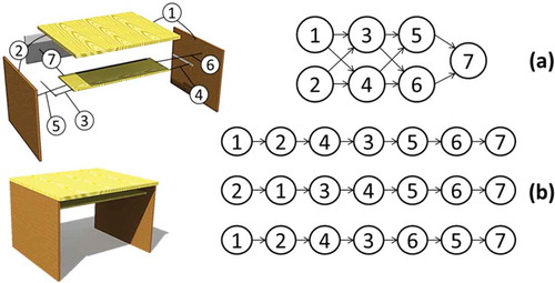
The advantage of generating precedence relations, rather than generating an assembly sequence directly, is that a precedence diagram contains more than one possible assembly sequence. This allows the selection of the most appropriate sequence based on additional assembly planning criteria, which can be applied in the different phases of assembly planning. For example, during process planning, alternative process times and costs can be calculated, which can help evaluate the different alternative sequences. Furthermore, additional constraints, beyond geometric, can be identified and included in the form of linked or incompatible tasks (Papakostas et al. 2014). However, the generation of precedence relations can be a complicated and time-consuming task, and since it is currently based on the engineers’ perception of the assembly, the results may exclude possible relations.

1.2. Assembly relations generation methods

The idea of assisting engineers in the process of generating an assembly sequence plan was a breakthrough that could reduce the time and cost of the planning and, as a result, the competitiveness of the manufactured products. Additionally, it could disengage the procedure from the necessity for an expert assembly sequence planner. Therefore, research has been carried out for generating assembly sequence plans automatically or semi-automatically.

A popular view on the generation of assembly relations was based on the following statement; ‘assembly by disassembling’. This statement was introduced in 1990 and is based on the fact that the knowledge of how a product is disassembled can provide the necessary information to assemble it (Lee and Shin 1990). This approach employed the contact-based feature to represent the precedence relationships of the product.

Later on, a model that generated assembly sequences by considering precedence relationships and different combinations of sub-assemblies was introduced (Ben-Arieh and Kramer 1994). The innovation of this approach was that a bigger assembly could be broken down into different sub-assemblies based on the proposed representation of the product. A novel approach regarding the modularisation of a product’s components utilising neural network algorithms and design structure matrices (DSMs) was also introduced by Pandremenos and Chryssolouris (2011). However, beyond the definition of a products’ structure and parts clustering, what is also necessary for the generation of assembly plans is the preliminary generation of precedence relations. All the precedence relations have to be converted to a graph frame, that is, precedence diagram, from which assembly plans can be generated. This method was adopted by some authors in order to generate a complete set of assembly sequences (De Fazio et al. 1990).

The two stages involved in this methodology were:

• The generation of the precedence relations between liaisons or logical combinations of liaisons in a mechanical product.

• The verification of the liaison sequence.

This methodology, however, required the precedence relations as input, the proper generation of which can be considered a time-consuming task. Regarding the direct assembly sequence generation methods, a number of approaches have been proposed in the recent years. Pan, Smith and Smith (2006) proposed a fully automated assembly sequence planner by directly extracting geometric information from STEP CAD files. In this approach, the geometric information to determine geometric assembly constraints was analysed and interference-free matrices were generated to represent spatial constraints between components during assembly operations. Chen and Liu (2001) created an adaptive genetic assembly planner that could find an optimal or near-optimal assembly sequence of a product. However, this approach required the pre-existence of geometric constraints information between the components of an assembly. Other approaches focused on the generation of disassembly sequences using software modules to generate disassembly constraints (Li, Wang, and Huang 2012).

In current industrial practices, after the definition of the assembly tasks and their relations, the tasks are further detailed and enhanced with additional subtasks. A common example concerns the condition that a component arrives to the line. A component might be outfitted in protective materials which require a ‘pre-task’ of removing them. Additionally, the engineers using methods-time measurement or similar methods determine the individual process times and define the relevant resources that have to be used (e.g. choosing between electric or pneumatic screwdrivers). Based on all this information, line balancing is performed, which concludes to the final assembly sequence, which, in a lot of cases, has parallel tasks. The main motivation for the work presented in this paper was the following:

• Current approaches for assembly sequence generation assume sequential tasks, which disregard parallel assembly choices or the regeneration of sequences from precedence diagrams (Gu and Yan 1995).

• Extraction of assembly information as early as the product design phase is currently complex and time-consuming. Moreover, the task of generating a precedence diagram in the industry is currently being performed using pen and paper methods and the correctness of the task sequences based on geometric constraints is initially dependent on the engineer’s perception.

• As modern customer trends move towards the personalisation paradigm, new assembly design methods in support of open product architecture and personalisation design need to be developed (Hu et al. 2011). These should be supported by tools that can extract production information fast.

2. Proposed approach

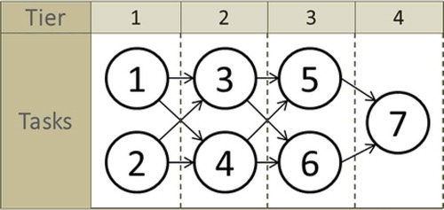
The proposed methodology introduces the concept of assembly tiers which correspond to different groups of parts or sub-assemblies of a product that can be assembled at the same time based on their geometric characteristics. In previous research work, the parallel disassembly groups have been described as assembly levels or layers for different applications (e.g. onion peeling; Chen et al. 1997). Assembly tiers can be considered as groups of parts that have to be assembled before or after other groups of parts. As an example of a tier, the desk used as an example in Section 1.1 has four assembly tiers (Figure 2).

Figure 2. Assembly tiers of desk example.

The proposed approach focuses on generating an assembly precedence diagram using assembly tiers. The proposed methodology includes the collision or clash identification between parts or sub-assemblies of the examined assembly as a core method. Furthermore, in order to complete the assembly task definition, the relevant fasteners are associated to the relevant parts or components. Finally, through an additional collision detection routine, the assembly tiers form the precedence diagram by identifying liaisons between parts of sequential tiers. In the generated diagram, each node is represented by a component and the links between these nodes represent assembly precedence relations.

Beyond some initial requirements that have to be satisfied for the CAD data to be processed, there are two steps where user input is required, which are only necessary at the start of the algorithm’s data processing and after the first results have been submitted to the user. The precedence diagram is provided to the user in the form of a spreadsheet containing all components and their precedence relations as well as their insertion directions to the assembly. The overview of the methodology can be seen in Figure 3.

Figure 3. Overview of algorithm’s steps.

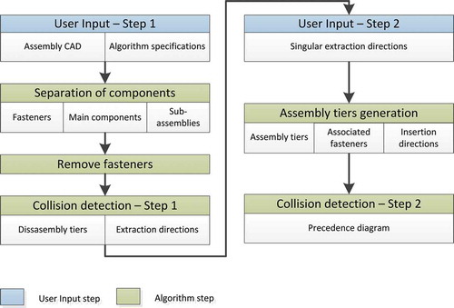
The different phases are described in the next sections. The two phases are separated by the two steps where input from the user is required.

3. Disassembly tiers generation

3.1. User input and CAD requirements

The first step of the methodology requires the user to provide the CAD data as well as specific parameters regarding the algorithms’ application. The CAD software used for developing the algorithm is CATIA V5-6R2013. Each product is represented by a CAD tree containing different levels of parts or assemblies. The algorithm identifies the components to be assembled as the components on the first level of the tree. Therefore, each component that will be pre-assembled should be on the first level and its parts or subcomponents on the second level. The algorithm can then be initiated as a Microsoft Visual Basic application.

After the algorithm has been initiated, the user is requested to select the assembly’s base component(s). These components will be considered being fixed, during the assembly processes, meaning that this may include additional assemblies representing fixtures. Furthermore, the user is prompted to provide a step for each component to be moved by during the algorithm’s collision tests as well as a value for the collision detection sensitivity.

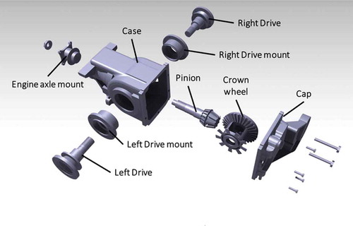
In order for the sequence of the algorithm’s steps to be demonstrated, a car differential (Figure 4) is presented. The assembly contains 16 components at its first level and the base component selected by the user is the ‘case’ component.

Figure 4. Exploded view of the differential assembly.

3.2. Separation of components

The separation of components into fasteners and assembly components is based on a previous methodology that identified the fasteners through their names (Ou and Xu 2013). The algorithm goes through the first level of the assembly, identifies the fasteners and deactivates/hides them. The fasteners are further separated into two groups: primary and secondary fasteners. The keywords used for identifying the primary fasteners in the current implementation are ‘bolt’, ‘screw’, ‘clip’, ‘wedge’ and ‘pin’, while for the secondary fasteners, the keywords are ‘nut’ and ‘washer’. The name identification is independent of the case that the letters of the name are provided (upper or lower). Finally, the rest of the components are separated into parts and sub-assemblies based on the tree hierarchy.

For the differential, the 16 components of the first level are separated into nine (9) assembly components, six (6) primary fasteners and one (1) secondary fastener. The primary fasteners are identified by the word ‘screw’ contained in their names (‘Screw1.1’, ‘Screw1.2’, ‘Screw1.3’, ‘Screw1.4’, ‘Screw2.1’ and ‘Screw2.2’). The secondary fastener is ‘Nut.1’ due to the keyword ‘nut’.

3.3. Fasteners removal and first collision detection

After the fasteners have been recognised and categorised into primary and secondary, they are removed from the scene (hidden) and their geometries are excluded from collision testing.

When the collision detection begins, the algorithm’s specifications for each part are calculated and stored. The specifications include the distance that each component has to be moved at different directions. The distances are defined based on the dimensions of the overall assembly. From these distances, a final position is calculated that the object must reach in a global or local axis without collision. If this occurs, then the algorithm recognises that the component can be removed from the assembly. As proposed by Ou and Xu (2013), additional directions are examined after a component has reached a position after which collision occurs. Based on possible constraints defined by the user during the design phase and are present in the CAD file, the possible directions that a component can be moved to are prioritised. For example, if there is an axis coincidence between two parts, both parts will be first checked for removal on this axis.

The following diagram shows the logical processes within the algorithm (Figure 5). The algorithm starts after the user has provided the input required and stops when no component has been left in the scene except the base component(s).

Figure 5. Collision detection algorithm.

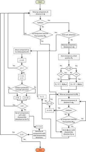
Where:

I: Total number of components that are in the scene minus the components selected as base parts. The total number of these components is reduced during the algorithm’s performance; when a tier has been identified, all components that belong to it are removed from the scene.

X: Set of all components that are not excluded as fasteners or user-defined base parts.

Where x_i ϵ X, i = 1, 2, 3….I.

S: The step (distance) that each component is moved to a certain direction when performing collision detection. The initial step is provided by the user (default value is set to 1 millimetre).

l: Number of current assembly tier. l = 1, 2, 3,…

D: Primary set of all axes (local and global) that a component can be moved at.

Each primary direction is denoted as d_j ϵ D, j = 1, 2, 3,…, 12, where d₁ = x_gl, d₂ = y_gl, etc. The sequence of the axes can change based on possible constraints defined by the user. All axes are checked, only if the ones that are prioritised on the basis of constraints do not provide an extraction path.

D₂: Secondary set of all directions (local and global) that a component can be moved at.

Each direction is denoted as d_2k ϵ D₂, k = 1, 2, 3,…, 10, where D₂ ⊂ D, since the axis that the component has already been moved at and the opposite axis are excluded from the secondary set.

The algorithm has the following steps:

1. The algorithm starts by moving a component at the primary directions defined by the local and global axes d_j (starting with x_gl) at a certain step (S), and then checks if the component has collided with any of the other components including the base components. If the local and global axes coincide, only the global axes are used. In the differential’s case, every component’s local axes system is parallel to the global axes system.

2. If a collision occurs after the first iteration, the algorithm stores the last position of the component that no collision occurred (P_ij).

3. Then the component is moved towards the secondary directions (d_2k) which are the same as the primary without the current d_j and its opposite.

4. At each component moving step of the algorithm, a final position is defined as explained earlier, which is different for the primary and secondary directions: P_Fij and P_Fijk, respectively.

5. If the object can reach any of the final positions without colliding with another object, then the primary axis d_j is stored as a valid disassembly direction. The same process is repeated until all primary axes have been checked.

6. Finally, after all components have been checked, the ones that can be disassembled at this stage (tier) are stored to the current tier (T_l) and removed from the scene.

7. If components remain in the scene (I > 0), the process is repeated until no components are left, except the base components.

The results of this process are the disassembly tiers as well as the possible disassembly directions/axes that a component can be extracted from the assembly. These are provided in a table containing one column per axis for the directions and one column containing the respective tier (Figure 6).

Figure 6. Output of the first collision detection step.

The form of the output of the first collision detection step for the differential is shown in Figure 7. It should be noted that the collision detection routine is not applied to the component ‘Casing.1’, since it is the base component and is indicated with a zero tier number.

Figure 7. Output of the first collision detection step for the differential.

4. Precedence diagram generation

4.1. User input for singular extraction paths directions

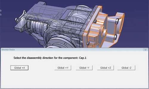
After the possible primary extraction directions have been generated, the user is prompted to select only one that will be used for generating the precedence diagram. If one or more extraction directions exist on the global axes, then the local axes are dismissed. The user is prompted for each component of the assembly, which in the implementation is highlighted, as well as the global or local axes he is expected to select one from. After the process has been completed, each component has only one extraction direction, which will later be inversed for the assembly precedence diagram generation. As seen in Figure 7, the only assembly component of the differential, with more than one extraction direction, is ‘Cap.1’. As a result, the user is prompted to select the appropriate extraction direction only for this component (Figure 16). During the implementation, the selected direction was X_gl.

4.2. Assembly tiers and associated fasteners

After the disassembly tiers and disassembly directions have been defined, the algorithm identifies the fasteners that are linked to each component. At the beginning of this step, all components are removed from the scene and the base components and fasteners are the only components left in the scene. Then, the components of each tier are reintroduced, one tier at a time, and moved one step (S) to their disassembly direction. When a fastener collides with a part, it is introduced into a new row under the moved component and removed from the scene. The component is then returned to its initial position. The whole process is repeated until all components of all tiers have been checked and therefore every fastener has been associated to a specific component. The following figure shows the processes of the algorithm (Figure 8).

Figure 8. Algorithm for fastener association to components.

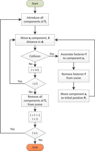
Where:

L:	=	maximum number of tiers.
di:	=	disassembly direction of component xi.
f:	=	fastener that collided with component xi.

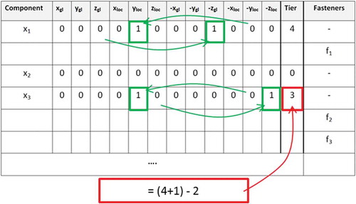
After the algorithm ends, each axis’ value that is 1 in the table presented in Figure 6 is set to zero and the opposite axis’ value is set to 1. Then the tier values are reversed except the base tier (T = 0) where the value of each tier is calculated as follows:

(1)

Considering the case of the differential, the translation of the disassembly tiers table in Figure 6 results in the assembly tiers table depicted in Figure 9.

Figure 9. Translation of disassembly tiers table to assembly tiers.

As seen in Figure 10, the component ‘Cap.1’ has collided with the six primary fasteners, showing that all six screws were attached to the cap of the differential. In addition, the component ‘Axle_mount.1’ has collided with the secondary fastener ‘Nut.1’ and thus is associated with it.

Figure 10. The translated disassembly tiers table to assembly tiers for the differential.

4.3. Association of components belonging to sequential tiers

Since each component that belongs to an assembly tier is associated through a precedence relation to one or more components belonging to the previous tier, these associations can be identified through collision detection. In this step, a component of a certain tier is tested for contact to a component of the previous tier, therefore generating a direct link between these two components. In the case where there is no direct connection to any component of the previous tier, a direct relation to all components of the previous tier is assumed. An example of this are the components, which are positioned inside a casing; the cap of the casing might have no collision to any of the enclosed components; however, there is a precedence relation to all components that are inserted last into the casing.

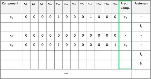
Finally, the components having as reference specific ones belonging to the assembly, the corresponding preceding components are added to the column ‘preceding components’. In Figure 9, the column ‘tiers’ is replaced with the column ‘preceding components’ (Figure 11).

Figure 11. Final precedence diagram table containing associated fasteners and insertion axes.

For the differential, each one of the two drives has the corresponding drive mount as the reference, as seen in the final precedence diagram table (Figure 12).

Figure 12. Final precedence diagram table of the differential.

In Figure 13, it can be seen that the ‘Nut.1’ fastener was associated to both the ‘Axle_mount.1’ and the ‘Pinion.1’ components (since both are joined by the nut). However, the first instance was disregarded as appearing in an earlier tier than the first one did. This means that the ‘Nut.1’ component will only be inserted after the ‘Axle_mount.1’.

Figure 13. Representation of the precedence diagram generated for the differential.

5. Implementation and case studies

The algorithm was developed as a macro application using the Visual Basic for Applications (VBA) embedded editor of CATIA V5-6R2013. The code is stored as a ‘.bas’ file and ‘.frm’ and ‘.frx’ files containing the input graphical user interfaces (GUIs) of the algorithm (e.g. when user input is required). The algorithm was initially tested using 13 product designs besides the differential. The CAD documents were set up based on the requirements of the algorithm; namely, the components to be assembled were all placed on the first level of the tree structure. All results were stored and presented to the user through an Excel sheet which is generated at the end of the algorithm by the macro application.

The collision detection was checked through the oClash.Compute function. At each time, two groups of components are checked, the one group contains the component that is being moved and the other one the components that are in the scene or belong to the previous tier, depending on the step of the algorithm that collision detection is performed (see Section 4.3). The sensitivity of the collision was dependent on the material of the component. More specifically, the materials considered were those found in the default material catalogue of the CAD application and could be used in components of industrial or mechanical products. These materials together with their elastic modulus values are presented in Table 3, according to the catalogue’s default categorisation. A collision detection sensitivity factor is used for each material in order to compensate for elastic deformations during assembly or disassembly. The factor of each material was selected on the basis of each material’s elastic modulus. The value of the collision detection’s sensitivity, which is defined by the user, is multiplied by the factor of each material. Therefore, the collision detection routine works different, based on the components that are being checked. The default and minimum value used is 0.5 millimetres (Abs(oConflict.Value) < 0.5) in order to ignore contacts.

5.1. Experiments

In order to obtain a better assessment of the algorithm’s efficiency, 13 product designs with diverse characteristics were used (Figure 14).

Figure 14. Product designs used in experiments.

The main characteristics that were taken into account for each product design were the total number of parts in all assembly tree levels, the number of components (distinct parts or sub-assemblies of parts) at the first level, the number of fasteners, the total volume of the assembly as well as its dimensions on the X, Y and Z axes. Finally, the total geometric elements of the assembly were recorded prior to the actual experiments in order to obtain a metric on the capacity required for the performance of collision checks Table 1.

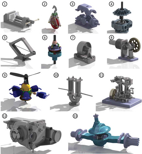
Table 1. Characteristic of product designs.

No.	Design	Total number of parts	Comp. on first level	Fasten.	Volume (m^3)	X dimension (mm)	Y dimension (mm)	Z dimension (mm)	Total geometric elements
1	Bench vice	16	10	6	2.97 × 10^−4	104	187	58	617
2	Crane hook	51	18	17	0.020	243	644	1082	1575
3	Gear box	19	19	0	5.27 × 10^−4	122	217	92	2417
4	Wankel engine	17	17	0	5.64 × 10^−4	69	63	82	2398
5	Mechanical jack	15	15	0	2.67 × 10^−4	101	450	224	836
6	Disc clutch	64	31	33	0.011	328	328	750	2847
7	Pulley fixing	11	7	4	0.020	230	150	198	457
8	Ramsbottom safety valve	25	21	4	0.0080	870	230	590	735
9	Stirling engine	41	17	20	4.76 × 10^−4	102	247	157	1272
10	Radial engine	115	27	76	0.044	1160	1136	1056	10,164
11	Steam engine	208	66	95	0.007	330	400	338	7798
12	Differential	19	12	7	0.005	400	230	354	5233
13	Rear axle	322	13	38	0.059	600	2059	696	6138

5.2. Results and discussion

The system used for the implementation of the case studies had the following specifications: Windows 7 Professional SP1 64-bit operating system, Intel(R) i7-2600 CPU 3.4 GHz, 8.00 GB installed memory (RAM) and NVIDIA GeForce GTS 450 1 GB GPU. The results with reference to time up to the assembly tiers’ generation can be seen in Table 2. The recording of the time started when the first component was moved, after the user had selected the base component(s) (Figure 15).

Table 2. Step used and results for each product design.

No.	Design	Step used (mm)	Number of tiers	Duration
1	Bench vice	5	4	0ʹ27”
2	Crane hook	10	8	1ʹ58”
3	Gear box	2	5	1ʹ21”
4	Wankel engine	2	5	1ʹ29”
5	Mechanical jack	5	3	0ʹ53”
6	Disc clutch	5	8	5ʹ05”
7	Pulley fixing	5	3	0ʹ19”
8	Ramsbottom safety valve	10	6	1ʹ09”
9	Stirling engine	5	4	2ʹ00”
10	Radial engine	10	6	6ʹ04”
11	Steam engine	5	8	20ʹ10”
12	Differential	10	4	1ʹ09”
13	Rear axle	10	3	7ʹ56”

Figure 15. Prompt box for the user to select base component(s).

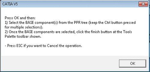
Table 3. Considered materials.

Material	Elastic modulus, E (GPa)	Suggested factor
Metal
Lead	16	1.5
Magnesium	44.81	1.2
Aluminium	70	1.2
Chroma	70	1.2
Silver	76	1.2
Gold	78	1.2
Zinc	97	1.2
Yellow brass	105	1.2
Bronze	110	1.2
Copper	110	1.2
Titanium	114	1.2
Brass	131	1.2
Steel	200	1
Iron	211	1
Nickel	214	1
Tungsten	400	1
Other
Rubber	2 × 10^−3	10
Plastic	2.2	5
Plexiglass	2.9	5
Epoxy	3	5
Raw polystyrene	3	5
Construction
PVC	3	5
Fabrics
Nylon	4	5

The experiments were performed through different steps during the collision detection phases, which covered the minimum width of the examined components. Some designs required no user input for the determination of extraction directions, since there was only one possible for each component, and as a result, the algorithm moved directly to the precedence determination and fasteners’ association. Some components required additional input, namely the differential, regarding the direction of the ‘Cap’ component that had five possible disassembly directions (Figure 16).

Figure 16. Disassembly directions for the ‘Cap’ component of the differential assembly.

The time taken by the user to select the directions was not included in the final measurements.

The results for all product designs can be seen in Table 2.

Although a direct link between characteristics and the algorithm’s duration cannot be obtained, it can be seen that the characteristics having a greater impact on the algorithm’s performance are the components at the first level as well as the geometric elements. However, it can be observed that for most designs, the algorithm’s duration was less than 2 minutes. In the case of the steam engine (66 components at the first level, 95 fasteners and 7798 geometric elements), it took the algorithm about 20 minutes to determine the precedence relations and fasteners’ association. It should be noted that in the current literature, there is no similar method providing the generation of the components’ precedence diagrams and the fasteners’ associations directly from CAD files. Therefore, a direct benchmarking of the algorithm’s performance is not feasible. However, it can be pointed out that the algorithm satisfies contemporary industrial needs considering that the actual time for the manual conception of the relevant information exceeds that of the algorithm.

6. Conclusions

The algorithm presented in this paper is used to generate assembly precedence diagrams of product assemblies directly from a product design’s CAD files. The novelty of the approach presented is the initial definition of assembly tiers, which defines groups of components that should be assembled sequentially. It should be stressed that the goal of this algorithm is not the generation of an optimum assembly sequence but rather all the possible sequences that can be used in later tasks of the assembly line design such as line balancing and parallel tasks definition. Existing approaches that use collision detection mostly concern sequence generation based on criteria that are not directly linked to the formation of assembly stations (e.g. cycle time and resources used). On the other hand, precedence diagrams generation approaches are usually performed through methodical user input such as detailed liaison graphs or AND/OR graphs. The approach presented in this paper tries to identify links among components after their sequential assembly groups have been defined in a mostly automatic approach.

The introduction of the assembly tiers concept aims at forming a basis for the further generation of assembly sequences or, in this case, precedence diagrams. Through this approach, the solution space for identifying the assembly relations of each component is reduced to the minimum possible, based on the geometric characteristics of the product. It was demonstrated that with existing technologies, even the ‘brute-force’ search for the identification of all assembly tiers can be performed in minutes providing quick support to the involved engineers. The second part of the algorithm performs selective search to identify the connections between components and fasteners and components belonging to sequential tiers. Future work will be focused on the addition of rotation of the components beyond their conventional moving on local and global axes as well as on the simplification of the collision detection routine through heuristics for the faster execution of the algorithm.

Acknowledgements

We would like to thank EDAG GmbH & Co. KGaA and Volvo Group Trucks Operations for their feedback.

Disclosure statement

No potential conflict of interest was reported by the authors.

Additional information

Funding

This study was partially supported by the projects Know4Car IP/FoF-ICT-2011.7.4 – 284602 and whiteR/FoF-NMP-2013-2 – 609228, funded by the European Commission.

References

- Ben-Arieh, D., and B. Kramer. 1994. “Computer-Aided Process Planning for Assembly: Generation of Assembly Operations Sequence.” International Journal of Production Research 32 (3): 643–656. doi:10.1080/00207549408956957.
- Bourjault, A. 1984. “Contribution a une approche méthodologique de l’assemblage automatisé: elaboration automatiquede séquences opératoires.” Thése d’état. Besançon, France: Université de Franche-Comté.
- Chen, S.-F., and Y.-J. Liu. 2001. “An Adaptive Genetic Assembly-Sequence Planner.” International Journal of Computer Integrated Manufacturing 14 (5): 489–500. doi:10.1080/09511920110034987.
- Chen, S.-F., J. H. Oliver, S.-Y. Chou, and -L.-L. Chen. 1997. “Parallel Disassembly by Onion Peeling.” Journal of Mechanical Design 119 (2): 267–274. doi:10.1115/1.2826246.
- Chryssolouris, G. 2006. Manufacturing Systems: Theory and Practice. 2nd ed. New York: Springer-Verlag.
- De Fazio, T. L., T. E. Abell, G. P. Amblard, and D. E. Whitney. 1990. “Computer-Aided Assembly Sequence Editing and Choice: Editing Criteria, Bases, Rules and Technique.” In IEEE International Conference on Systems Engineering 1990, 416–422. doi:10.1109/ICSYSE.1990.203185.
- Eng, T.-H., Z.-K. Ling, W. Olson, and C. McLean. 1999. “Feature-Based Assembly Modeling and Sequence Generation.” Computers & Industrial Engineering 36 (1): 17–33. doi:10.1016/S0360-8352(98)00106-5.
- Gu, P., and X. Yan. 1995. “CAD-Directed Automatic Assembly Sequence Planning.” International Journal of Production Research 33 (11): 3069–3100. doi:10.1080/00207549508904862.
- Homem de Mello, L. S., and A. C. Sanderson. 1990. “AND/OR Graph Representation of Assembly Plans.” IEEE Transactions on Robotics and Automation 6 (2): 188–199. doi:10.1109/70.54734.
- Hu, S. J., J. Ko, L. Weyand, H. A. ElMaraghy, T. K. Lien, Y. Koren, H. Bley, G. Chryssolouris, N. Nasr, and M. Shpitalni. 2011. “Assembly System Design and Operations for Product Variety.” CIRP Annals - Manufacturing Technology 60 (2): 715–733. doi:10.1016/j.cirp.2011.05.004.
- Lee, S., and Y. G. Shin. 1990. “Assembly Planning Based on Geometric Reasoning.” Computers & Graphics 14 (2): 237–250. doi:10.1016/0097-8493(90)90035-V.
- Li, J., Q. Wang, and P. Huang. 2012. “An Integrated Disassembly Constraint Generation Approach for Product Design Evaluation.” International Journal of Computer Integrated Manufacturing 25 (7): 565–577. doi:10.1080/0951192X.2011.646310.
- Ou, L.-M., and X. Xu. 2013. “Relationship Matrix Based Automatic Assembly Sequence Generation from a CAD Model.” Computer-Aided Design 45 (7): 1053–1067. doi:10.1016/j.cad.2013.04.002.
- Pan, C., S. S. Smith, and G. C. Smith. 2006. “Automatic Assembly Sequence Planning from STEP CAD Files.” International Journal of Computer Integrated Manufacturing 19 (8): 775–783. doi:10.1080/09511920500399425.
- Pandremenos, J., and G. Chryssolouris. 2011. “A Neural Network Approach for the Development of Modular Product Architectures.” International Journal of Computer Integrated Manufacturing 24 (10): 879–887. doi:10.1080/0951192X.2011.602361.
- Papakostas, N., G. Michalos, S. Makris, D. Zouzias, and G. Chryssolouris. 2011. “Industrial Applications with Cooperating Robots for the Flexible Assembly.” International Journal of Computer Integrated Manufacturing 24 (7): 650–660. doi:10.1080/0951192X.2011.570790.
- Papakostas, N., G. Pintzos, C. Giannoulis, N. Nikolakis, and G. Chryssolouris. 2014. “Multi-Criteria Assembly Line Design under Demand Uncertainty.” In 8th International Conference on Digital Enterprise Technology, March 25–28. Stuttgart, Germany: Procedia CIRP, 25, 86–92.
- Rekiek, B., A. Dolgui, A. Delchambre, and A. Bratcu. 2002. “State of Art of Optimization Methods for Assembly Line Design.” Annual Reviews in Control 26 (2): 163–174. doi:10.1016/S1367-5788(02)00027-5.
- Riggs, R. J., and S. J. Hu. 2013. ‘Disassembly Liaison Graphs Inspired by Word Clouds.’ Procedia CIRP 7: 521–526. doi:10.1016/j.procir.2013.06.026.