Machine configuration and workload balancing of modular placement machines in multi-product PCB assembly

ABSTRACT

A popular gantry-type placement machine includes several interconnected, autonomously operating component placement modules and the machine was designed so as to able to use different kinds of placement heads and vacuum nozzles in the modules, which can be easily changed. Although this increases the flexibility of the production line, the reconfiguration phases of the modules may be unproductive and one should keep them to a minimum. In addition, the production times can be shortened by balancing the workloads of the machine modules. Here, a two-step optimisation method for the machine reconfiguration and workload balancing in the case of multiple Printed Circuit Borad (PCB) batches of different sizes and PCB types is presented. The objective is to minimise the total production time, and keep the machine configuration the same for all batches. The proposed algorithm is iterative and it applies integer programming for the workload balancing along with an evolutionary algorithm that searches for the best machine configuration. In experiments, for single PCB types the proposed algorithm obtained optimal or near optimal solutions. For multiple PCB types the solutions favour the PCB types that have a bigger production time due to greater batch sizes, but the total production time is still close to optimal.

KEYWORDS:

• Printed circuit board
• modular machines
• machine configuration
• mixed-model workload balancing
• integer programing
• genetic algorithm

1. Introduction

In the electronics industry, the assembly of electronic components on Printed Circuit Boards (PCBs) is a crucial task consisting of several consecutive phases where the stations are interconnected by a conveyor belt mechanism (Hayrinen et al. 2000; Johnsson and Smed 2001). These include the dispension of the glue or paste for fixing the electronic components on the bare PCB, the actual placements of the components to their proper positions, the final fixing of the components using an oven and testing the functionality of the PCB. Since the design of the boards varies, production volumes are generally large and high precision is needed, this will require the use of automatic assembly machines. To increase productivity, assembly lines are constructed from several placement machines working in parallel, which may be tailored to handle components of different shapes. It is typical that the component placement operation of surface-mounted electronic devices is the most time-consuming step of the assembly process. Recent component placement machines operate in pick-and-placement cycles, where each cycle collects a number of components from a component feeder unit to the vacuum nozzles of the placement head, moves the head to the proper positions where the components will be inserted on the PCB, and finally returns to the feeder area to pick up the next set of components. In addition to these basic steps of the pick-and-placement cycles, the machine checks prior to the actual placement operation the identity and orientation of each component on the fly or by using of an extra camera. The mechanical movements between the PCB and the feeder unit and between the placement points on the PCB cause time delays which increase the time needed for the placement mechanism. In some cases it is also necessary to change some nozzles in the placement head during the assembly process. This is a time-consuming operation which should in general be avoided. Last, when moving to a new PCB type the feeder, head and nozzle settings demand manual intervention in the production process, which has an impact on the overall efficiency of the production process. While the characteristics of the mounting machines may vary, the machine types can be classified into five main categories (Ayob and Kendal 2008). These are a dual delivery machine, where pick-and-place operations alternate between the two sides of the machine, there are two arms, and while one is placing components the other can pick up new ones; multi-station machine (or modular machine), where several placement modules are connected via a conveyor belt and the modules operate autonomously; turret-type machine (chip shooter), where a rotating turret (operating like a carousel) holds a number of nozzles that are filled with components at a fixed pickup position and then placed in a fixed placement position, the PCB table moves in the X or Y direction and the feeder unit in the X-direction; multi-head machine (pick-and-place or collect-and-place machine) has an X-Y gantry used to move components from the feeder unit to the PCB. The PCB table and the feeder unit may or may not be moveable; sequential pick-and-place machine, where the arm holds only one nozzle. Otherwise, the organisation is just like that for the multi-head machine case.

One of the most popular variants of the above machine types today is the modular gantry-type placement machine. Here, each of the machine modules contains a feeder unit that holds the reels or trays of different component types and a moveable arm that is installed in an X-Y gantry. The arm is equipped with a replaceable rotary placement head for holding several changeable nozzles (see, e.g. Fuji NXT or Siemens Siplace) (Kallio, Johnsson, and Nevalainen 2012). The PCB table and the feeder unit are static and the multi-head placement arm operates in pick-and-place cycles. For each cycle, the arm picks up the required components into the nozzles from the feeder unit, and then moves to the PCB area to put them into their placement positions. The head is rotated such that an appropriate nozzle is above the feeder reel (or placement point) when picking up (or placing) the component. The main advantage of this type of machine is that the configuration is flexible, since the feeder unit, head and nozzles can be adjusted to the requirements of the product type. Furthermore, the gantry-type operation is accurate and relatively simple compared to that of a moveable PCB table and feeder unit structure.

To improve the production rate and help maintain the competitiveness of the company, the goal of production planning and control is to increase the number of manufactured (fault-free) products (per unit time) with low equipment cost and operating cost. Therefore, two key objectives in production planning and control are to reduce the number of machines (or modules of a modular machine) in the line and at the same time to speed up production. Sometimes both aspects appear in the objective as a weighted combination (see the Simple Assembly Line Balancing Problem of type E (SALBP-E) described in Scholl and Becker (2006)). In the electronics industry, the machine line is usually designed for a long production planning period so the number of modules is fixed and the efficiency is improved by increasing the production rate.

The method for designing the production process depends on the characteristics of the assembly lines, machine types, the number of product types and the similarity of the products (Becker and Scholl 2006). The problem of optimising a PCB assembly process may be divided into several different phases. For a definition of eight subproblems, see Crama, van der Klundert, and Speiksma (2002). These are

1. the assignment of PCB jobs to product families and families to lines;

2. the allocation of components to machines;

3. partitioning the component placements for each machine;

4. sequencing the jobs on each machine;

5. the arrangement of the feeders in feeder units;

6. the sequencing of the component placements;

7. determining the feeders for retrieval of the components; and

8. controlling the movement of the heads above the placement area.

The present study focuses on component-to-machine module allocation and component placement partitioning problems on a single assembly line (problems 1–3), while the remaining problems (4–8) are put to one side here. What makes this study different from previous research (for a survey on assembly line balancing, see Battaia and Dolgui 2013)) is that the machine modules can be easily reconfigured. This useful property allows one to have a more flexible design, but it also increases the complexity of production planning.

The case where only one PCB type is produced without the need to change, the set-up of the line is called the single-model case. In practice, there are usually several product types to be assembled on the same line. Here, when the products are sufficiently similar to be manufactured without reconfigurating or changing the set-up of the machine line, the production is known as the mixed-model strategy. However, if the assembly line requires any changes in the set-up (feeder allocation, head assignment, nozzle assignment) during production, the products need to be grouped into families so that a machine set-up operation (or reconfiguration) is performed only between any two families (Smed et al. 1999; Ho, Ji, and Dey 2008). This case is called the multi-model strategy.

When the batch sizes of different PCB types are small, the reconfiguration of a modular machine during the assembly process takes up a great proportion of the total time required to manufacture the products. It is then better to have a general configuration for all PCB types (where possible) and to allocate the workload to the machine modules for each product types in a balanced way. In the present study, this kind of scenario is examined for the machine module configuration and line balancing. Here, a set of PCB batches is handled on a single modular gantry-type machine (i.e. a machine consisting of several independently operating machine modules). The problem is really a subproblem of organising all the assembly operations on a whole production line, which commonly includes (for reasons of efficiency) some other assembly machines. Then, the general question is how to efficiently allocate the placements to all machines of the line. To answer this question, one has to handle the low-level optimisation problem, i.e. the optimal use of the modular placement machine. In order to do this an abstraction is needed to find the solutions of phases 4–8 (see above). Here, the order of component reels in the feeder unit and the placement sequences are not discussed, but the placement time of the module varies linearly with the number of placements. Next, the component-to-machine module allocation and component placement partitioning optimisation problem is divided into two sub-problems; namely finding an efficient module-configuration and balancing the workload among the modules.

Although the mixed-model case is examined in the present study, the configuration problem for modular placement machines also appears in the single model machine set-up strategy; but in the latter without any machine set-ups between the jobs (Toth, Knuutila, and Nevalainen 2010; Rong et al. 2011; Guo et al. 2012). The same problem also appears in different forms in other branches of industry; see Boysen, Fliedner, and Scholl (2008) for some example application areas. For instance, the organisation of mass production in the automobile industry has been studied in detail; see Oliveira et al. (2012).

The line balancing of three or more machines is a well-known NP-hard problem for the single-model (Guthjar and Nemhauser 1964) and mixed-model (Thomopoulos 1967) cases. There are many solution methods available for the simple assembly line balancing problem, called SALB, where the machines are identical (Scholl and Becker 2006), and the general assembly line balancing case, called GALB (Becker and Scholl 2006; Bentaha, Dolgui, and Battaia 2015) The main difference between PCB assembly line balancing and general line balancing is that in the electronics industry the precedence among the component placements is not so important and it is usually ignored. However, for PCB assembly the characteristics of the placement machine modules (especially capacity constraints) and the compatibility rules between the equipment (head, nozzle) and the component types are more complex. The solution approaches available for the single-model case employ exact methods (Baybars 1986) and heuristics (Ayob and Kendal 2008). For the mixed-model case, the solution methods include integer programing (Thomopoulos 1970), branch-and-bound (Bukchin and Rabinowitch 2006), Lagrange relaxation (Lapierre, DeBargis, and Soumis 1998) and heuristics (Crama et al. 1998; Simaria and Vilarinho 2004; Ho, Ji, and Dey 2008; Akpinar, Bayhan, and Baykasoglu 2013). In these studies, the line configuration and machine set-up are fixed. While this is a valid assumption in many real-life manufacturing facilities, the current modular reconfigurable placement machines have been designed without this assumption so as to offer more flexibility in the usage of resources for component placement. This provides the motivation for this present study. Owing to the flexibility of the machine reconfiguration, a reconfigurable modular machine is not a fixed resource, but its efficiency depends on the set-up of the modules. This issue should be taken into account when balancing the workload of the line. However, in some article the configuration is partly considered. For example see Lin, Lin, and Huang (2016) and Luo, Liu, and Hu (2017) where nozzle assignment is also optimised.

The Machine Configuration and (Work) Load Balancing (MCLB) problem for modular gantry-type placement machines was originally discussed by Toth, Knuutila, and Nevalainen (2010) for one product type. In this case, the machine reconfiguration and load balancing are performed for each job change. The optimisation of these tasks is a computationally hard problem and, moreover, reconfiguration needs to be performed manually. Here, the MCLB problem is generalised to the multi-product case, called Machine Configuration and (Work) Load Balancing for Multiple products (MCLB-M). Another difference with the MCLB is that in the present study, instead of a single nozzle type, there may be several different optional nozzle types by which a component can be assembled. This feature adds both flexibility and complexity to the production planning. However, this problem is occurred when a modular placement machine is used for a set of different job batches, each having its own demands of resources (nozzles, heads and component reels); and, in order to save on machine set-up time, the whole set of batches should be produced with the same configuration of the modules. At first glance, the problem could be trivially solved by creating a super PCB that covers all the resources from the individual PCB types. Of course, the generated configuration is feasible for the original problem too, but the workload balancing may be very poor since the balancing problem needs to be solved individually for each PCB type. Furthermore, the impact of different batch sizes would not be then taken into account and the solutions would turn out to be unsatisfactory. As an extreme case, suppose that the batch sizes of two PCB types are 1 and 10,000. Then the machine configuration should favour the latter PCB type (Salonen et al. 2006).

The two sub-problems (the configuring and balancing of the MCLB-M) are closely interconnected. In Rong et al. (2011), a joint mathematical model was presented for the single job case (MCLB) and solved in an optimal way for small instances. The approach is, however, too time-consuming for real-world problem sizes. To overcome this difficulty, an algorithm is proposed for the MCBL-M where the two problems are solved separately; the previous solution to the one sub-problem is iteratively applied as an input for the next one. As this approach is a heuristic, we cannot guarantee finding the optimal solution. Here, a hybrid metaheuristic is given which combines a genetic algorithm for generating the machine line configuration and an integer programming solution for the line balancing sub-problem. To the best of our knowledge, the MCLB-M problem for the mixed-model production case has not been discussed before in the literature. The solutions are evaluated by determining the estimated total assembly time of the production plans of a set of single PCB problems and also on generated random multi-product problems. It transpires that the results of the algorithm are optimal or close to an optimal solution in the single PCB-type case and it works well for multi-model cases, too.

In Section 2, the MCLB-M problem is defined more precisely and a mathematical model is presented in Section 3. The solution method is introduced in Section 4, then in Section 5 the computational results are presented. Last, we summarise our findings and make some suggestions for future research.

2. Problem definition

2.1. Reconfigurable modular component placement machine

In the following, the operation principle of a modular PCB component placement machine is examined. This machine type is also called a reconfigurable modular component placement machine, or simply a (reconfigurable) modular machine (Figure 1).

Figure 1. A gantry-type placement machine with three identical configurable modules. Each module has a single gantry mechanism, multi-nozzle head and a feeder unit.

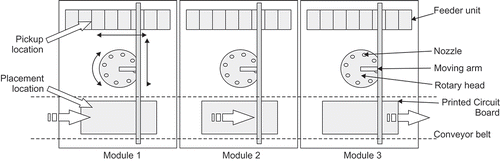
The component assembly process of each module of a gantry-type machine performs a (simplified) set of actions. These are the following:

1. The head moves to the feeder unit area.

2. It picks up the required components into its nozzles one at a time.

3. It moves above the stationary PCB.

4. It places the components into the board one at a time, and

5. it returns to the feeder unit area.

6. Steps 2–5 are repeated until every assigned component has been inserted into the board.

The operations for automatically replacing the nozzle have been omitted here because they are in practice avoided as they are too time-consuming in medium and small batch size assembly manufacturing processes, like the one considered here.

When a module of a machine has finished its task with a PCB, the product can be moved forward to the next module of the same machine or to the next machine of the production line. Obviously, the fully connected conveyor belt must wait before moving until every module of the machine and every other line machine has finished its task (paged production line). The time between two successive moving steps is called the cycle-time and it is defined by the slowest machine module (called the bottleneck machine module) in the line. The cycle-time commonly varies among different products.

In the MCLB problem, the following input data are given (see Tables 1 and 2). Here, the machine line contains m reconfigurable modules. Each module is supposed to be of the same (gantry-) type that has a changeable placement head which can hold several vacuum nozzles. There are in total h head types and n nozzle types. In the study, it is assumed that there is a sufficient number of heads and nozzles of every type. A compatibility relation is defined between the head types and nozzle types (i.e. each head type is related to a set of compatible nozzle types, where HN_ij denotes the compatibility of head type i and nozzle type j) and in a similar way, between the component types and the nozzle types (i.e. each nozzle type is related to a set of component types which it can handle, and AN_jk denotes nozzle type j and component k). Each head type i has a capacity C_i, i.e. the maximal number of nozzles it can hold. Each machine module has its own feeder unit (also called the component magazine). The feeder unit has a capacity F representing the number of slots needed for storing the component reels. The capacity is the sum of the component tape widths in the feeder unit and it cannot be exceeded. It is supposed that each placement head requires a certain (average) time to pick an electronic component from the feeder unit and put it into the board. This is called the pick-and-place time, which may vary for different head types (T^pp_i with head type i). What is more, the average travelling time is defined for each head type, which includes the time of checking using a camera (T^tr_i with head type i). This is the average time needed by the head to move from the feeder unit area to the board and back. These two time factors determine the speed of a head.¹

Table 1. Inputs.

M	Set of machine modules
m	m = |M|
H	Set of head types
h	h = |H|
N	Set of nozzle types
n	n = |N|
A	Set of component types
a	a = |A|
B	Set of PCB types
b	b = |B|

Table 2. Parameters.

HNij	1 If head type i is compatible with nozzle type j, 0 otherwise
ANjk	1 If nozzle type j is compatible with component type k, 0 otherwise
Ci	Capacity of head type i (i.e. the maximal number of nozzles in the head)
F	Capacity of feeder unit (i.e. the number of component reel slots)
Wk	Width of component reel of type k (in slots)
T^ppi	Average pick-and-place time of head type i
T^tri	Average travelling time of head type i
Pq	Batch size of PCB type q
Rqk	Number of placements of component type k on PCB type q

2.2. Machine configuration and (work) load balancing for multiple products (MCLB-M)

The problem formulation of MCLB-M is a generalisation of the MCBL for the single PCB type case (Rong et al. 2011). Now, the production plan includes b PCB types and a different component types in total. Each component type i has a width W_i, i.e. the number of slots in the feeder unit occupied by the component reel. For each PCB type q the production plan gives the batch size P_q, i.e. the number of PCBs of the same type to be produced, and the number of placements R_qk of each component type k is also given.

The goal of the MCLB-M problem is to determine, for a given set of PCB types with known batch sizes, a joint machine module configuration and a component-to-machine assignment fulfilling the compatibility and capacity constraints such that the estimated total processing time of the production plan is minimal.

The machine configuration means the head assignment to machine modules, the nozzle assignment to the heads and the feeder allocation (i.e. which component types are inserted into the feeder units of the modules, omitting the order of the reels). A machine configuration is said to be feasible for a PCB type if the board can be produced on it. This means that there is at least one machine module for each component type that has a compatible nozzle fixed to the placement head of the module and the feeder contains the component type. A machine configuration is called feasible for the production plan if it is feasible with all PCB types in the production plan.

In a feasible machine configuration, the machine set-up is fixed for the whole production plan so none of the head assignments, the nozzle assignments or the feeder allocations of any machine module must be altered during the production phase. This design avoids the need for the manual intervention of the machine set-up and break time caused by it. To minimise the total operation time, the machine configuration and the allocation of the components to the modules must be designed such that the assembly of each PCB type is as swift as possible, taking into account the batch sizes of the products (i.e. PCB types).

For a feasible machine configuration, the task is to assign the component placements of the PCB types to the nozzles of the different modules in such a way that the workload of the bottleneck module (i.e. where the workload is maximal) is minimised. The question of component-nozzle compatibility, the feeder allocation and the operation time must then be considered when the components are being assigned.

2.3. Example

For the parameter settings of a sample configuration see, Table 3.

Table 3. Configuration parameters of a sample MCLB-M problem.

Number of machine modules, m	4
Number of head types, h	3
Number of nozzle types, n	7
Number of component types, a	10
Capacity of feeder unit, F	20
Capacities of head types, Ci (i = 1 to 3)	3 2 1
Widths of the component types, Wi (i = 1 to a)	1 2 3 4 5 5 6 7 8 8
Average travelling times of head types, T^tr	1 1 2
Pick-and-place times of head types, T^pp	1 2 3
Component-Nozzle compatibility matrix, AN (a × n)	1 0 0 0 0 0 0 1 1 0 0 0 0 0 1 1 0 0 0 0 0 0 1 1 0 0 0 0 0 1 1 0 0 0 0 0 0 1 1 0 0 0 0 0 0 1 1 0 0 0 0 0 0 1 0 0 0 0 0 0 0 1 1 0 0 0 0 0 0 1
Head-Nozzle compatibility matrix HN (h × n)	1 1 1 0 0 0 0 0 0 1 1 1 0 0 0 0 0 0 1 1 1

In the compatibility matrices, the value of an element is 1 if the corresponding component type and nozzle type (AN_jk) or head type and nozzle type (HN_ij) are compatible, and 0 if they are not. For example, in Table 3 the first row of the HN-matrix means that head type 1 is compatible with nozzle types 1, 2 and 3, but not compatible with any one of nozzle types 4, 5, 6 and 7.

3. Mathematical model

Using the above notations, a mathematical formulation can be given for the MCLB-M problem. The following variables are defined for the head-to-module, nozzle-to-head, component-to-feeder and placement-to-module assignments.

mhli	=	equals 1 if head type i is assigned to machine module l
falk	=	equals 1 if component type k is assigned to the feeder unit of machine module l
hnlj	=	denotes the number of nozzles of type j is assigned to the head of machine module l
maqkl	=	stands for the number of component of type k is assigned to machine module l in the case of PCB type q

The constraints of the model are the following:

(1)

(2)

(3)

(4)

(5)

(6)

(7)

(8)

(9)

(10)

(11)

(12)

(13)

The first three formulas define the capacity bounds. Constraint (1) states that exactly one head must be assigned to each machine module. Constraint (2) states that the total width of the component reels assigned to the feeder unit of each module must not exceed the feeder capacity. Constraint (3) states that the number of nozzles assigned to the head of each module is equal to the capacity of the head. The following three types of constraints are needed for maintaining the compatibility rules. Constraint (4) states that any nozzle can be assigned to a head if they are compatible and, similarly, constraint (5) states that a component placement can be assigned to a machine module if its head contains at least one compatible nozzle. Constraint (6) states that a component placement can be assigned to a module if its feeder unit contains the reel of the component type. Constraint (7) states that precisely the required number of placements assigned to the modules. Constraints (8) and (9) state that a component reel is assigned to the feeder unit or nozzle to the head if there is at least one component placement assigned to the corresponding machine module that needs it. Last, constraints (10)–(13) characterise the domains of the variables.

To evaluate a feasible solution of the MCLB-M problem, the slowest machine module has to be found for each PCB type because the bottleneck modules define the cycle times of PCB types. For a given module, the operation time depends on the number of pick-and-place cycles made by the head. To determine this value is not a trivial task as it depends on the configuration of the machine module and the assigned component placements. For each component, there may be more than one compatible nozzle in the head and one nozzle can handle several different component types; and the number of cycles depends on the load of the nozzles in the head. Therefore, the assigned placements must be balanced among the nozzles which leads to a new optimisation problem. Moreover, this subproblem can be resolved only when the characterisation of the module (i.e. the head and the nozzles in the head) is fixed. Not surprising, there is no exact mathematical formulation which can give the precise production time when the machine configuration and the workload balancing are optimised together.

For the MCLB-M, the production time can be estimated using lower and upper bounds. In the worst case, only one nozzle in the head can pick and place all the assigned component placements, which means that number of cycles of the head is then equal to the number of placements. Therefore, this value can be used to define an upper bound for the production time of one PCB. In the best case, the component placements are equally balanced among the nozzles of the head and the number of cycles can be calculated by dividing the number of placements by the head capacity and rounding up the result. One possible way of estimating it is to use a weighted combination of these upper and lower bounds. The weight could express the quality of the optimisation process for an individual module. Formally, let RM_ql be the total number of placements of PCB type q assigned to machine module l.

(14)

The estimated number of cycles by the head of module l for PCB type q is then the following:

(15)

where w_ub and w_lb are the weights for the lower and upper bounds. The production time for machine module l and PCB type q can be estimated by applying the following formula:

(16)

Using the above values, the bottleneck module can be defined for PCB type q and the production time of a single board can be computed.

(17)

Then, the objective function corresponds to the minimisation of the total production time for the production plan. That is,

(18)

4. Multi-model evolutionary algorithm (MEA) for module configuration and balancing

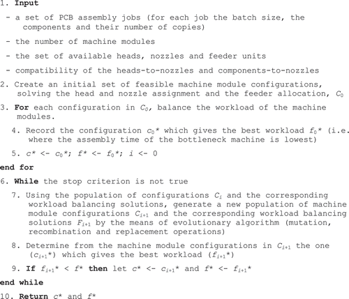
As shown in Section 3, an exact mathematical formulation for the MCLB-M problem is not easy to provide and an exact way of solving it is not known. Furthermore, in the article by Rong et al. (2011) it was found that their integer programme for an easier problem was hard to solve and advanced techniques for traversing the solution space are required. In addition, the solution time of the model was very large for bigger problem instances. For these reasons, sub-optimal solutions are sought here by dividing the MCLB-M into two sub-problems. Namely, (1) generating a common feasible machine module configuration of the head assignment, nozzle assignment and feeder allocation for all the jobs; and (2) creating a component-to-module assignment for each PCB type that minimises the estimated total production time of the whole production programme. An evolutionary solution method is applied here, called the Multi-model Evolutionary Algorithm (MEA) (see Figure 2). First, a machine configuration is generated for the modules. Then, since only one PCB type is produced at a time, the line balancing (including the component assignment to all line machines) is solved independently for each PCB type. Next, the solution is evaluated by using the estimated manufacturing time of the whole production plan. For a fixed feasible machine module configuration, the workload balancing problem is handled using a linear IP method. To look for good configuration candidates, an evolutional algorithm (EA) is applied due to it having provided excellent results for the basic MCLB problem (Toth, Knuutila, and Nevalainen 2010). The EA codes the candidate solutions in a natural way, and includes efficient operations for generating new solutions.

Figure 2. Multi-model Evolutionary Algorithm (MEA) for machine module configuration and line balancing.

The initial population of module configurations is generated by a greedy method (see Section 4.1). The algorithm is based on the same basic idea as that in (Toth, Knuutila, Nevalainen 2010), but now the generalised nozzle-head and component-nozzle compatibility must be considered in the nozzle-to-head and nozzle-to-component assignments. The integer programming model for the evaluation of the component assignment (i.e. workload balancing of component placements) is described in Section 4.2. The details of the evolutionary algorithm are discussed later on in Section 4.3.

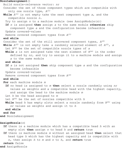
4.1. Initial population of machine module configurations

A component type is compatible with a machine module if there is at least one compatible nozzle in its head and there is enough spare capacity in the feeder to store it. A configuration covers a component type a_k if there is at least one machine module that is compatible with component type a_k. For each machine module, each component type has a covered value, which is the number of compatible nozzles in the head of the machine. A machine configuration is thus compatible with a PCB type if it has a positive covered value for all component types of the board.

Head and nozzle assignment (step 2). First, those component types that are compatible with only one nozzle type are considered sequentially. For a component of this kind, a nozzle is inserted greedily into the first compatible head (which has been already assigned to a machine module). If there is no head for the component, then a compatible head type with the highest nozzle relevance (see below) is assigned to an empty machine module. The new nozzle is then assigned to the new head. If, however, there is no empty machine module, the component type is just skipped, resulting in an infeasible machine configuration. These component types are ignored in the later steps for this configuration, but are incorporated into the evaluation by using a penalty value (see later). Recall that here an assigned nozzle may cover more than one component type.

For the second step of the initial configuring process, each uncovered component type is compatible with more than one nozzle type. To select one of these nozzle types, a new parameter is introduced called the nozzle-relevance (nr). Its value describes how many component placements can be carried out with this particular nozzle type relative to the total number of component placements R in the whole production plan.

(19)

where

(20)

To maintain the configuration diversity, the uncovered component types are covered in a random order. (Recall that a set of different configurations will be generated to form an initial population of candidate solutions of MEA.) For each uncovered component type, a compatible nozzle with the highest nozzle-relevance value is assigned to a machine module. The assignment process is the same as that above for the first step. If this action is not possible, the next compatible nozzle types are tried out in the order of decreasing nozzle relevance values.

When all component types have been covered with at least one nozzle, the remaining empty slots of the heads are filled with extra nozzles. As it was said before, to increase the diversity of the configurations, a probability factor is used for nozzle selection, i.e. a nozzle with high nozzle-relevance is selected with a higher probability than a nozzle with low nozzle-relevance. If there is a machine module without any assigned head, a nozzle is selected in the same way as before, the head with the highest capacity compatible with the selected nozzle being assigned to the machine module, and the head is filled with nozzles in the same way.

For the pseudo code of the initial head and nozzle assignment method, see Figure 3.

Figure 3. Pseudo code for initial nozzle assignment.

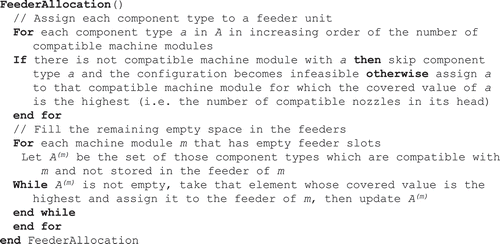
Feeder allocation (steps 2 and 7). The component types that are not yet stored in any feeder unit are assigned in ascending order according to the number of compatible machine modules. Using this sequence, each component type is greedily assigned to the feeder unit of the compatible machine module with the highest covered value. Clearly, when a component type is assigned to a feeder, some other component types may become incompatible with that module because there is no longer sufficient space in the feeder. This process is repeated until every component type has been assigned to some feeder and then the configuration is feasible for all jobs. If a component type cannot be assigned to any feeder, it is skipped and the configuration is deemed infeasible.

Since a component type may be compatible with more than one machine module, putting the component into as many feeder units as possible should increase the likelihood to achieve a more balanced workload. Hence, the remaining free capacity of the feeder units is filled in the following way. For each machine module, a list of the compatible component types not yet in its feeder is generated. The list is created in order of the covered values. The component types are assigned to the feeder unit in this order until the feeder unit is filled or there are no compatible component types left. The process is repeated for each machine module.

For the pseudo code of the feeder allocation, see Figure 4.

Figure 4. Pseudo code of the feeder allocation.

Workload balancing (steps 3 and 7). As outlined in Section 3, to evaluate a solution of the MCLB-M problem, it is not enough to balance the component placements among the machine modules, because it is also necessary to assign the components to the nozzles. Since in the workload balancing phase, the machine configuration is already given the component-to-nozzle assignment of the heads is possible here. The machine configuration is given by:

mh(l)	=	the head type assigned to machine module l
fa(l,j)	=	1 if component type j is assigned to the feeder unit of machine module l, 0 otherwise
hn(l,j)	=	the nozzle type assigned to the jth place (i. e. nozzle location) of the head in machine module l

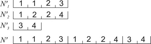
Let N’_l be the list of the assigned nozzles ordered by their nozzle locations in the machine module l and N’ a catenation of the N’_l lists (see Figure 5). Note that these structures are multi-sets of nozzle types, as more than one copy of a particular nozzle type can be inserted into a head.

Figure 5. Nozzle list (N’) of three machine modules.

Since a component type may be compatible with several different nozzle types, it is hard to determine the number of feeder-PCB-feeder tours made by the head. Because a nozzle can hold only one component at a time, the head must go there and back as many times as there are component placements assigned to any particular nozzle. Thus, the number of cycles performed by the head is determined by the maximum load of its nozzles.

An infeasible machine configuration does not cover some component type. To increase the chance that these component types become covered in the next iteration of MEA, the relevance value (nr) of those nozzle types is increased, which are compatible with the uncovered component types. For each uncovered component type, the nozzle-relevance value of each compatible nozzle is simply multiplied by a constant greater than one (a value of 1.5 was used in our tests). A higher nozzle-relevance value increases the probability of fitting a compatible nozzle to a module, and with a greater number of compatible nozzles it is more likely that one can successfully assign the component type to the feeder unit.

4.2. Integer programming formulation for workload balancing

To evaluate a feasible configuration (for steps 3 and 7 of MEA), the component placements of each PCB type have to be assigned to the machine modules such that the production time is minimised.

Production times of the different modules turn out to be unequal due to the compatibility constraints caused by the settings of feeders, heads and nozzles. For a fixed machine module configuration the load balancing must be solved for each PCB type and these individual balancing problems are independent of each other. This is why they can be handled one at a time or even simultaneously via parallel computation. Therefore, the following formulation is applied for each PCB type.

The mathematical model presented in Section 3 is modified in such a way that the configuration is fixed and thus the corresponding constraints are removed. Two new variables are presented and the constraints of the workload balancing are modified according to the nozzle setting N’. For PCB type q, the integer variable s_ql gives the number of pick-and-place cycles of the head in machine module l. Variable na_qkj gives the number of placements of component type k assigned to the nozzle j (∈N’). Next, Q is a big constant.

For each PCB type q∈B,

(21)

where

(22)

(23)

(24)

(25)

(26)

The objective function defined in (21) minimises the processing time of the slowest machine module. Constraint (22) states that every component placement must be assigned to some nozzle for each component type. Constraint (23) tells us that a component placement can only be assigned to a compatible nozzle. Constraint (24) states that placements of a component type can be assigned only to the nozzles of a module that has the component type in its feeder. Constraint (25) states that for each machine module, the load of every nozzle is smaller than or equal to the number of pick-and-place cycles of the head. Last, constraint (26) gives the permitted domains for the variables.

A standard way to linearise a minmax objective function is to introduce a new variable τ that denotes the maximum processing time, replace the objective one that minimises τ and provide new constraints to each machine module that ensure that their processing times are less than or equal to τ. With this modification, the new objective function is

(27)

and the new set of constraints is

(28)

The model was implemented in Java and solved using CPLEX (version 11.1).

4.3. Genetic algorithm for machine configuration

The optimisation of the machine configuration is a complex task and involves exploring a large search space. For industrial-sized problems, it introduces unacceptable running times if one has to find a globally optimal solution. In the following, the genetic algorithm (GA) framework (Holland 1975) is applied to look for a set of good feasible solutions for the machine module configuration problem (steps 6 to10 of MEA). GA is based on a population of individuals, where each of them represents a candidate solution. With a fitness function, the individuals are evaluated and compared to each other. With two operations, the recombination and the mutation, new individuals called offspring, are created from selected individuals called parents. During the replacement process, the members of the next generation are selected from the pool of the candidate individuals. The GA then iterates until a stopping criteria is met (see Michalewicz (1996) for details). Here, the basic concepts of our algorithm are the following.

4.3.1. Individuals

An individual represents a configuration of the machine modules. An individual is coded as (1) an integer vector containing the head assignment to the machine (mh(l) gives the head type in machine l); (2) an integer matrix containing the nozzle assignments to the heads (hn(l,j) gives the number of nozzles of type j in the head of machine l); and (3) a binary matrix which defines the feeder allocations of the modules (here, fa(l,k) is 1 if component type k is in the feeder of machine module l).

4.3.2. Fitness

To evaluate a configuration, the component placement time is calculated for each different PCB type (see Section 4.2 above). If the machine configuration is feasible for a PCB type, the production time of the PCB batch is added to the global fitness value. Otherwise, a penalty term is added to the global fitness:

(29)

where T^PR_q is the production time of PCB type q which is found by solving the corresponding workload balancing subproblem defined by the integer programme (21)–(28); y_k is 1 if a component type k is missing from the component assignment and 0 otherwise; K_q is a penalty and P_q is the batch size for PCB type q. To calculate the penalty, it is supposed that each missing component type will be handled by the slowest head and each placement requires one complete cycle by the head. The value of the penalty is defined as the total number of component placements of board q multiplied by the longest travelling time and longest pick-and-place time.

(30)

where h’ is the head type with the longest travelling time and h’’ is the head type with the longest pick-and-place time. In this way, the GA allows infeasible solution candidates, but makes them unfavourable.

4.3.3. Mutation

The mutation operation increases the diversity in the population by making random changes in the individuals. In our model, the mutation works on the head and nozzle assignment. For each machine module, the operation with a predefined low probability changes the head and assigns the nozzles to the head using the nozzle-relevance values (see Section 4.1). In the case where the head is not changed, the mutation is executed on the nozzles. Then, with the same probability each nozzle is changed to another compatible nozzle type that is selected by the roulette-wheel selection technique (see Michalewicz 1996) using the nozzle-relevance values.

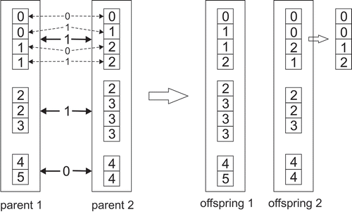
4.3.4, Recombination

The role of recombination (or crossover) is to generate new configurations by mixing the characteristics of two selected individuals. The machine modules of two individuals are considered pairwise and for each pair a random crossing is performed. First, a bit vector v (v_l, l = 1 to m) is randomly generated to define the swapping positions. The module pairs are considered in increasing order of l. If v_l = 0, then the pair is bypassed. Otherwise, if the head types of the two modules are different, they are simply swapped with their nozzles and feeders. If, however, the head types are the same, for each nozzle location the assigned nozzles are swapped using another random bit vector w (w_j, j = 1 to C_mh(l)). Then the feeders are reallocated for both machines, as was done for the initial configuration (see Section 3.1).

After this procedure, the heads and nozzles are reordered by their indices. For an example, see Figure 6 below.

Figure 6. A recombination operation on two sample configurations with 3 machine modules, 3 head types (capacities 4, 3, 2) and 6 nozzle types. The Boolean vector for modules is v = (1 1 0) and Boolean vector for nozzles of module 1 is w = (0 1 0 1). In offspring 2, the first head is then sorted by the nozzle identifiers.

4.3.5. Replacement

The pool of candidate solutions contains the individuals of the previous generation and the generated offspring. Linear ordering selection is then used to select the individuals for the next generation, i.e. the individuals are sorted according to their fitness values and the required number of best individuals (size of the population) is chosen that will survive and become the next generation.

4.3.6. Parameters

Evolutionary algorithms have many parameters and various methods have been proposed for adapting the operations of the general model to the needs of the current optimisation problem (Eiben, Hinterding, and Michalewicz 1999). Therefore, these parameters were determined by a tuning process where each parameter was determined independently. A set of values was defined for these parameters. Each value was tested one by one on randomly generated problem instances of different sizes and the best parameter value was kept. To select the number of individuals in the generation (i.e. the population size), four options were tried out (5, 10, 20 and 50) and the population size of 20 gave the best results. For our problem instances, tests demonstrated that a higher population size did not improve the solutions significantly, but did increase the running time. In each generation, the mutation operations were performed on each individual. The best probability of changing a head or nozzle in the configuration turned out to be 0.2, which was chosen from the set {0.05, 0.1, 0.2. 0.3, 0.4, 0.5}. The number of recombination operations performed was equal to the population size. For the selection of the parents, the random, 2-tournament and roulette-wheel selection methods were tested. Out of these, the roulette-wheel method produced the best results. For the new generation, the best individuals were selected by using the linear ordering of their fitness value taken from the pool of the members of the previous generation and the new offspring. This method actually performed better than the 2-tournament and roulette-wheel selection methods. The stopping criterion was the maximum number of the generations, which here was set to 1000. This value was sufficient for the problems studied here. For more information about EA methods, see Michalewicz (1996).

5. Computational results

The MEA optimisation method was implemented in Java and executed on an Intel i7 3.6GHz, 8GB computer; and the integer programming problems were solved by using the CPLEX software package. The performance of MEA was evaluated on two different sets of problem instances. For efficiency evaluations, the problem instances were taken from Toth, Knuutila, and Nevalainen (2010) and Rong et al. (2011). In the article by Toth, Knuutila, and Nevalainen (2010), a metaheuristic for a single product MCLB (which is called SEA) was presented and its efficiency was evaluated by Rong et al. (2011) by solving the corresponding IP programme. Even though the algorithm in the present study was constructed for the production of several PCB types, its efficiency can be analysed on single PCB as well. To evaluate the MEA for multi-model production, random problem instances were generated that represent real-life industrial products of different sizes.

5.1. Single job problems

The algorithm was tested with the single PCB production problems (see Table 4) published by Toth, Knuutila, and Nevalainen (2010) and Rong et al. (2011). The results of the MEA were compared to the results of SEA and the optimal solution.

Table 4. Basic parameters of problem instances in single PCB cases.

	Component types	Machine modules	Head types	Head capacities	Nozzle types	Feeder capacity	Placements
1	8	5	2	4, 1	5	10	55
2	8	4	2	4, 1	5	12	74
3	10	5	3	8, 4, 1	8	20	100
4	20	8	4	8, 4, 2, 1	10	30	320
5	40	8	4	12, 8, 4, 1	15	30	525

The results in Table 5 show that the proposed algorithm works quite well for these problem instances. The production time is equal or close to the global optimum found by means of the IP-programme formulation. With travelling time 1 for problem instance 5 and with travelling time 10 for instances 4 and 5, the optimal production time is not known because these instances were too large for the integer programing method (Rong et al. 2011). Nevertheless, the resulting values of MEA are lower than those found using the single-model evolutionary algorithm SEA.

Table 5. Summary of test results for the problem instances of Table 4 with traveling times 1 and 10.

	T^tr = 1					T^tr = 10
	Production time (sec)					Production time (sec)
	OPT	SEA	RT (sec)	Gen	MEA	OPT	SEA	MEA	RT (sec)	Gen
1	39	39	39	26	0.55	84	85.3	84	83	5.4
2	78	78	78	11	0.25	166	168.6	167.8	15	0.85
3	96	96.7	96	38	26.4	150	156.7	151.5	66	4.4
4	120	121	120	5671	180.3	-	198.6	192	4646	107.3
5	-	264.8	261.25	4941	68.4	-	388.7	365.9	6483	164.4

The results are averages of 20 independent runs. The production times of the proposed multi-model evolutionary algorithm (MEA) are compared to the optimal (OPT) given by Rong et al. (2011) and the previously published single-case evolutionary (SEA) solutions in Toth, Knuutila, and Nevalainen (2010). The other columns list the running time of MEA in seconds (RT) and the number of those generations (Gen), where the final solution was found by MEA (the 0th generation stands for the initial generation). For the bigger problem instances, the optimal solutions are not known.

5.2. Generation of random PCB products

To the best of our knowledge, there are no available benchmark data for the MCLB problem. However, the design of real-life products is protected by the owner companies and not permitted to publish it. Therefore, to evaluate the method developed here in the multi-model case, randomly generated test instances were used which reflect the characteristics of real products. For generating test instances, a statistical analysis was performed based on real-life industrial data. The production database contains 341 different PCB types and 410 component types. The size of the products varies from small to large, i.e. from only a few component placements to hundreds on the PCBs. In order to generate a similar data set the database was analysed and two different frequency values were defined for each component type. The first one, called freq_ct(k) (for each k∈A) represents the frequency of the component type k which describes the probability that component type k is needed for a PCB. This value is calculated by using the number of those PCB types that use component type k divided by the total number of PCB types. The other frequency value, called freq_pl(k) (for each k∈A), represents the frequency of the number of placements from component type k. It provides the probability that a component placement of a PCB is taken from component type k, assuming that the component type is used for this product. This value is defined using the average of the number of placements of the component type k divided by the total number of placements, taking into account those PCBs that use component type k.

To generate the problem instances, two parameters are used. Namely, (1) the size of the product (R), i.e. the number of placements; and (2) the range of the required component types, i.e. how many different component types can be used (at least (a_min) and at most (a_max)) for the generated PCB (R ≥ a_max).

A sample set of PCBs is then generated as follows. First, the algorithm randomly generates a component type list for the instance in the following way. The number of component types (a) is randomly selected from the defined interval (a_min ≤ a ≤ a_max) and a random order of the component types is created. Component type k is taken from the order and a random number λ is generated (0 ≤ λ ≤ 1). If freq_ct(k) ≥ λ, component type k is added to the component list. This process is then continued until the number of selected component types is equal to a. If every possible component type has been checked and some types are still needed, a new order of the unselected component types is generated and the process is repeated.

In the second phase of the instance generation, the placements are selected randomly using the component types in the list. First, one placement is added to the product taken from each component type. The rest of the placements are then selected using a method similar to a roulette wheel selection. A wheel is constructed by the frequency of component placements (freq_pl), where each component type has a sector whose size is proportional to its frequency value. A sector is randomly selected from the wheel and one placement is added from the selected component type to the PCB. This method is repeated until the required number (R) of component placements have all been added.

5.3. Multiple jobs, multipurpose nozzles

To test the algorithm in the multi-model case, the problem instances used were of three different sizes; namely small, medium and large. Each generated problem instance contains ten different PCB types of equal batch size. Here, the parameters of the configuration are defined by considering the problem size. Also, the multi-model production is relevant when the cost of the module reconfiguration is high compared to the cost of the production. This may be due to the small batch sizes or the similarity of the PCB types. For two product types which share most of the required component types, a common configuration can give acceptable production times for both products. In order to assess this kind of production plan, a relatively small set of component types (see the second column of Table 6) was used to generate PCB types and the generator chose a number of required component types for each PCB (see the last column of Table 6).

Table 6. Parameter values for the generated test instances.

	Component types	Machine modules	Head types	Head capacities	Nozzle types	Feeder capacity	R	amin-amax
I	25	3	2	4,1	4	16	50	20–25
II	25	4	3	8,4,1	6	16	100	20–25
III	50	6	3	8,4,1	6	20	250	35–45

Row I stands for small instances, row II for medium and row III for large. Columns from the second to sixth indicate the parameter values of the machine configuration. The last two columns are for the parameter values of the generated product types. The seventh column contains the number of placements and the last column gives the minimum value and maximum value for the number of required component types for a certain PCB type.

To evaluate the results, two lower bounds were used for the MCLB-M. The first lower bound tells us something about the configuration. The idea is that a common configuration of the whole production plan is usually not optimal for each PCB type individually. If the machine configuration is handled separately for each job, the configurations may be better suited to the different PCB types, and in this way, provide lower production times. So MEA was run for each PCB type individually and the sum of the resulting production times was used as the first lower bound. This value gives the cost for a problem instance as if the machine line had been reconfigured with zero cost after each PCB type batch. Note that MEA does not always find the global optimum of the single product MCLB, but the result is still lower. The other lower bound is valid only for identical batch sizes based on a relaxation of the problem in the workload balancing phase. The value of the bound is the production time of the ‘Super PCB’ which contains all the component placements of every PCB in the problem instance. In this way, the multi-model problem may be simplified to the single product case. Since the batch sizes are the same for each PCB type, the machine line places exactly the same set of components into the Super PCB as it does with the original PCBs with batch sizes 1. Hence, the generated configuration is as good for the Super PCB as it is for the set of original PCBs. However, the total workload may be more balanced for the Super PCB case than for the single PCB case processed one by one. For example, when producing the Super PCB, one module inserts the components of one PCB type while another module inserts the components of another PCB type at the same time. This case cannot happen with the originally separated product types since the different PCB types are assembled one after the other. Here, the higher value of the two bound is used as a global lower bound.

For each problem instance of Table 7, twenty independent runs were made with the Super PCB and with the single PCBs independently. The best solutions of these runs were then used as the lower bounds. Twenty runs were made with the original multi-model problem instances and the averages of the resulting production times were used for the evaluation of MEA.

Table 7. Results obtained using MEA in the multi-model case of random generated test instances got by averaging twenty independent runs.

	Production time
	MEA	Single	Super	Gap (%)	RT (sec)	Gen
Small_0	305	301	297	1.3	217.5	19
Small_1	306	299	297	2.3	219.7	23
Small_2	302	289	293	3	204.5	14.6
Small_3	300	287	293	2.3	193.9	15.7
Small_4	301	292	290	3	205	18.8
Small_5	307	288	293	4.6	193.6	18.9
Small_6	303.3	295	294	2.7	200.4	12.3
Small_7	307.2	301	298	2	189.5	11.1
Small_8	309	281	298	3.6	192.6	13.6
Small_9	299.7	298	293	0.6	210.8	13.3
Medium_0	369	369	361	0	572.8	21.3
Medium_1	378.8	378	367	0.2	540.4	13.5
Medium_2	370.5	346	363	2	643.5	36.7
Medium_3	368	368	362	0	595.6	21.9
Medium_4	372	353	363	2.4	549.8	13.7
Medium_5	371	370	363	0.3	623	29.1
Medium_6	374	366	364	2.1	494.9	1.6
Medium_7	372	372	362	0	517.4	4.5
Medium_8	371.6	371	364	0.2	624.8	30.2
Medium_9	369	369	360	0	512.4	9.4
Large_0	692.8	553	683	1.4	1575.6	57
Large_1	690.2	545	680	1.5	1691.6	68
Large_2	691.9	535	685	1	1385.9	43.7
Large_3	569	543	558	1.9	1583.4	21.5
Large_4	691.3	553	682	1.3	1543.3	56
Large_5	694.3	547	684	1.5	1761.1	75.2
Large_6	692	552	682	1.4	1724.4	67.4
Large_7	688	560	682	0.9	1306.6	28.3
Large_8	692.1	553	682	1.5	1338.9	33.3
Large_9	693.9	552	685	1.3	1590.1	59.4

The first column is the problem instance, while the second is the resulting production time by MEA. The next two columns give the lower bounds for production time, where the Single column comes from the single job production and the Super from the production time of the Super PCB. The Gap column lists in percentage terms the differences between the results of MEA and the global lower bounds (the higher of the two lower bounds). Next, the last two columns list the running time (RT) and the number of generations (Gen) required for MEA to get the final solution.

The results in Table 7 show that MEA is strong and robust for smaller and larger product types, even when there are several different PCB types in the production plan. It can be seen that for almost every problem instance, the difference between the production time of MEA and the lower bound is at most 3%. However, for larger problem instances (i.e. with a bigger number of modules and components) the running time of MEA increases. Though the number of iterations of the evolutionary algorithms increases slightly, the higher running times are mainly caused by the larger line balancing problems, which are solved by the IP-solver.

When several PCB types are assembled with a common configuration, the algorithm configures the assembly line by taking into consideration their batch sizes. To test this feature of MEA, production programmes of the PCB types of Table 7 were generated by varying the batch sizes of the jobs. For this test, four medium-sized PCB types were used. First, the batch sizes were given the same value and then the batch size of one board was set to twenty times that of the others. The resulting production times are shown in Table 8.

Table 8. The production time of PCB types in different production plans.

Batch size				Production time
PCB1	PCB2	PCB3	PCB4	PCB1	PCB2	PCB3	PCB4	Total	Single	Super
1	0	0	0	62	-	-	-	62	62	-
0	1	0	0	-	50	-	-	50	50	-
0	0	1	0	-	-	44	-	44	44	-
0	0	0	1	-	-	-	70	70	70	-
1	1	1	1	75	54	75	100	304	226	304
20	1	1	1	62	75	67	100	1482	1404	1729
1	20	1	1	90	50	90	100	1280	1176	1330
1	1	20	1	62	75	67	100	1577	1520	1729
1	1	1	20	79	107	91	70	1677	1556	2204

The four leftmost columns list the batch sizes, while the next five columns show the resulting production time for each PCB type and for the total production plan. In the next column, a lower bound (Single) is given for the production plan which is calculated from the single product times, and the rightmost column contains the production time using the configuration generated for the Super PCB.

The results in Table 8 show that the MEA algorithm efficiently adjusts the machine line configuration according to the proportion of the product types. When the production plan contains more than one PCB type with equal batch sizes, the generated configuration is designed in such a way that the production time of each PCB type increases smoothly and uniformly (see the middle row). However, if the batch sizes of the PCB types are different, the configuration is adjusted so as to reduce the assembly time of larger batches, usually at the expense of the others. Nevertheless, the total production time is still close to a lower bound, which is calculated using the individual production times of the PCB types. If a Super PCB is utilised instead of the individual PCB types, the generated configuration is not good when the batch sizes are different (see the values in columns ‘Total’ and ‘Super’). It can also be seen that the feasible configurations are also strongly affected by the design of the boards defined in the production plan.

The objective function of MEA contains a penalty term that which helps one to create feasible machine configurations. The method for generating the initial configuration attempts to cover every component type by solving the head and nozzle assignment first and then the feeder allocation. Therefore, some component types might still remain uncovered. This happens when too few nozzles and too few modules cover the component type and the feeder capacity of these modules is not big enough for all the required components. The nozzle-relevance updating (see Section 4.1) increases the covering probability of these component types by raising the relevance-value, i.e. the number of the compatible nozzles in the configuration. This is why the algorithm tends to generate feasible solutions, and if it finds at least one the final solution will be feasible.

When solving the multi-product MCLB problem in two phases (i.e. determining the machine configuration and balancing the workload), adding new PCB types to the production plan does not make the problem more difficult for MEA. The parameter set of the machine configurations defines the search space of the problem. The feasibility of a machine configuration for a set of PCBs depends on the number of different components in terms of the machine capacity (i.e. the number of modules, feeder sizes, nozzle types, head capacities) and not on the number of different PCB types. Because the different configurations are evaluated by the manufacturing time of the global production plan, the task of exploring the search space just depends on the configuration parameters and not on the number of different PCB types. Also, the workload balancing is solved separately for each PCB type. However, the running time of MEA increases with the number of the PCB types since more workload balancing subproblems must be solved for each iteration of MEA.

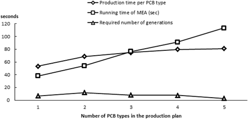
To test the above points, a set of production plans was generated that contained a different number of PCB types ranging from 2 to 5 (see Table 2). For groups with two PCB types, pairs were generated for all the combinations of the PCB types; for groups with three PCBs every triple was generated, etc. Here, the batch of each PCB type has the same size. For each test, the same configuration parameters of the modules were used (see Table 1) and the results were averaged over twenty independent runs. Figure 7 tells us that the average running time of MEA increases linearly with the number of PCB types. However, the average number of generations did not change much in these tests. It is also apparent that the production times of the individual PCB types increase slightly when the number of different PCB types is bigger in the production plan. This is because MEA has to balance the assembly time of the different PCB types to conform to the generated configuration of the machine modules. The result of the balancing then depends on the similarity of the different PCB types in the group.

Figure 7. The effect of the number of different PCB types on the average production time per PCB type, the average running time of MEA and the average number of generations (where the final solution was first found by MEA). The x-axis gives us the number of PCB types in the production plan. The results are averages of 20 independent runs with all possible PCB type combinations for each number of different types (i.e. one PCB type, two PCB types, etc.).

The running time of MEA depends on the time needed to generate the initial population (t_init), the number of iterations (n_it) and the time for an iteration (t_it). That is

(31)

Out of these, t_it has a polynomial time dependence for production, and the time needed to solve the workload balancing problem can be found using IP. This latter problem is NP-hard and the solution got by using the CPLEX package that may be very time consuming. However, in our tests the times were found to be acceptable.

6. Conclusions

The machine configuration and the workload balancing of reconfigurable gantry-type machine modules were studied for the case where the production programme includes several different product types and the machine configuration is kept fixed for a set of PCB job batches of different sizes. Compatibility relations were defined between heads and nozzles and between nozzles and components such that n-to-m relations are permitted. The present problem is new and the proposed algorithm can be integrated into a complex system for managing the set-up, balancing and machine control of one or several assembly lines.

Since any change in a line configuration is time consuming, an efficient machine configuration is crucial for a lower manufacturing time and it is also needed when the production plan consists of several different product types. The component assignment of the MCLB-M differs from the traditional assembly line balancing problem as the compatibility constraints are much more complicated, but the precedence restrictions among the operations performed for the PCBs are usually omitted. In this study, an iterative metaheuristic MEA was presented for solving the MCLB-M problem. The heuristics used a genetic algorithm to generate new line configurations and an integer programming model for the line balancing.

The efficiency of MEA was demonstrated by comparisons with optimal solutions and with an earlier published heuristic algorithm in the single product case. To test MEA in the multi-model case, several randomly generated problem instances were utilised. The results indicate that MEA works well for hard problems as well. The good adaptivity of the algorithm was demonstrated in a multi production case by varying the batch sizes of different PCB jobs. Because MEA optimises the estimated total production time, it gives higher weights to the PCB types that require more time due to their complexity or batch size. However, when the number of different component types becomes large there is naturally no guarantee that a feasible machine module configuration will be found or that it is even possible.

In real-life PCB manufacturing, it is quite common that the production plan contains so many and such different products that they cannot be assembled without a reconfiguration of the machine line. In future research, our plan is to improve the presented algorithm in such a way that it groups the products and sequences the groups efficiently and then solves the MCLB-M for each group. Another possibility is to allow some (automated or manual) nozzle changes during the assembly process.

Disclosure statement

No potential conflict of interest was reported by the authors.

Notes

1. While this kind of approximation looks unrefined, it turns out to be reasonable in tests (Vainio et al. 2014). More sophisticated machine models (Kallio, Johnsson, and Nevalainen 2012) exist, but they would need extra data, which are not available in the module reconfiguration and load balancing phase. Here, the ordering of the nozzles in the head, the topology of the PCBs, the ordering of the component types in the feeder unit and the sequence of the component placements have been omitted. A consideration of these points would introduce new hard combinatorial optimisation subproblems (Crama, Van Der Klundert, and Speiksma 2002).

References

- Akpinar, S., G. M. Bayhan, and A. Baykasoglu. 2013. “Hybridizing Ant Colony Optimization via Genetic Algorithm for Mixed.Model Assembly Line Balancing Problem with Sequence Dependent Setup Times between Tasks.” Applied Soft Computing 13: 574–589. doi:10.1016/j.asoc.2012.07.024.
- Ayob, M., and G. Kendal. 2008. “A Survey of Surface Mount Device Placement Optimization: Machine Classification.” Europian Journal of Operational Research 186 (3): 893–914. doi:10.1016/j.ejor.2007.03.042.
- Battaia, O., and A. Dolgui. 2013. “A Taxonomy of Line Balancing Problems and Their Solution Approaches.” International Journal of Production Economics 142: 259–277. doi:10.1016/j.ijpe.2012.10.020.
- Baybars, I. 1986. “A Survey of Exact Algorithms for the Simple Assembly Line Balancing Problem.” Management Science 32 (8): 909–932. doi:10.1287/mnsc.32.8.909.
- Becker, C., and A. Scholl. 2006. “A Survey on Problems and Methods in Generalized Assembly Line Balancing.” European Journal of Operational Research 168: 694–715. doi:10.1016/j.ejor.2004.07.023.
- Bentaha, M. L., A. Dolgui, and O. Battaia. 2015. “A Bibliographic Review of Production Line Design and Balancing under Uncertainty.” 15th IFAC Symposium on Information Control Problems in Manufacturing — INCOM 2015, Ottawa, Canada, Vol. 48, 70–75.
- Boysen, N., M. Fliedner, and A. Scholl. 2008. “Assembly Line Balancing: Which Model to Use When?” International Journal of Production Economics 111: 509–528. doi:10.1016/j.ijpe.2007.02.026.
- Bukchin, Y., and I. Rabinowithc. 2006. “A Branch-And-Bound Based Solution Approach for the Mixed-Model Assembly Line-Balancing Problem for Minimizing Stations and Task Duplication Cost.” European Journal of Operation Research 174: 492–508. doi:10.1016/j.ejor.2005.01.055.
- Crama, Y., O. E. Flippo, J. van de Klundert, and F. C. R. Spieksma. 1998. “The Assembly of Printed Circuit Boards: A Case with Multiple Machines and Multiple Board Types.” European Journal of Operational Research 98: 457–472. doi:10.1016/S0377-2217(96)00228-7.
- Crama, Y., J. van der Klundert, and F. C. R. Speiksma. 2002. “Production Planning Problems in Printed Circuit Board Assembly.” Discrete Applied Mathematics 123: 339–361. doi:10.1016/S0166-218X(01)00345-6.
- Eiben, A. E., R. Hinterding, and Z. Michalewicz. 1999. “Parameter Control in Evolutionary Algorithms.” IEEE Transactions Evolution Computation 3: 124–141. doi:10.1109/4235.771166.
- Guo, S., K. Takahashi, K. Morikawa, and Z. Jin. 2012. “An Integrated Allocation Method for the PCB Assembly Line Balancing Problem with Nozzle Changes.” The International Journal of Advanced Manufacturing Technology 62: 351–369. doi:10.1007/s00170-011-3803-7.
- Guthjar, A. L., and G. L. Nemhauser. 1964. “An Algorithm for the Line Balancing Problem.” Management Science 11 (2): 308–315. doi:10.1287/mnsc.11.2.308.
- Hayrinen, T., M. Johnsson, T. Johtela, J. Smed, and O. S. Nevalainen. 2000. “Scheduling Algorithms for Computer-Aided Line Balancing in Printed Curcuit Board Assembly.” Production Planning & Control 11 (5): 497–510. doi:10.1080/09537280050051997.
- Ho, W., P. Ji, and P. K. Dey. 2008. “Optimization of PCB Component Placements for the Collect-And-Place Machines.” International Journal of Advanced Manufacturing Technology 37: 828–836. doi:10.1007/s00170-007-1014-z.
- Holland, J. H. 1975. Adaptation in Natural and Artificial Systems. University of Michigan Press.
- Johnsson, M., and J. Smed. 2001. “Observations on PCB Assembly.” Optimization, Electronic Packaging & Production 41 (5): 38–42.
- Kallio, K., M. Johnsson, and O. S. Nevalainen. 2012. “Estimating the Operation Time of Flexible Surface Mount Placement Machines.” Production Engineering 6 (3): 319–328. doi:10.1007/s11740-012-0380-z.
- Lapierre, S. D., L. DeBargis, and F. Soumis. 1998. “Balancing Printed Circuit Boards Assembly Line Systems.” International Journal of Production Research 38: 3899–3911. doi:10.1080/00207540050176076.
- Lin, H. Y., C. J. Lin, and M. L. Huang. 2016. “Optimization of Printed Circuit Board Component Placement Using an Efficient Hybrid Genetic Algorithm.” Applied Intelligence 45: 622. doi:10.1007/s10489-016-0775-1.
- Luo, J., J. Liu, and Y. Hu. 2017. “An MILP Model and a Hybrid Evolutionary Algorithm for Integrated Operation Optimisation of Multi-Head Surface Mounting Machines in PCB Assembly.” International Journal of Production Research 55 (1): 145–160. doi:10.1080/00207543.2016.1200154.
- Michalewicz, Z. 1996. Genetic Algorithms + Data Structures =Evolution Programs. 3rd ed. Berlin: Springer.
- Oliveira, F. S., K. Vittori, R. M. O. Russel, and X. L. Travassos. 2012. “Mixed Assembly Line Rebalancing: A Binary Integer Approach Applied to Real World Problems in the Automotive Industry.” International Journal of Automotive Technology 13: 940–993. doi:10.1007/s12239-012-0094-4.
- Rong, A., A. Toth, O. S. Nevalainen, T. Knuutila, and R. Lahdelma. 2011. “Modeling the Machine Configuration and Line-Balancing Problem of a PCB Assembly Line with Modular Placement Machines.” The International Journal of Advanced Manufacturing Technology 54 (12): 349–360. doi:10.1007/s00170-010-2920-z.
- Salonen, K., J. Smed, M. Johnsson, and O. Nevalainen 2006. “Grouping and Sequencing PCB Assembly Jobs with Minimum Feeder Setups.” Robotics and Computer-Integrated Manufacturing 22, 4, August 2006: 297–305. doi:10.1016/j.rcim.2005.07.001.
- Scholl, A., and C. Becker. 2006. “State-of-the-Art Exact and Heuristic Solution, Procedures for Simple Assembly Line Balancing.” European Journal of Operational Research 168: 666–693. doi:10.1016/j.ejor.2004.07.022.
- Simaria, A. S., and P. M. Vilarinho. 2004. “A Genetic Algorithm Based Approach to the Mixed-Model Assembly Line Balancing Problem of Type II.” Computer & Industrial Engineering 47: 391–407. doi:10.1016/j.cie.2004.09.001.
- Smed, J., M. Johnsson, M. Puranen, T. Leipala, and O. S. Nevalainen. 1999. “Job Grouping in Surface Mounted Component Printing.” Robotics and Computer-Aided Manufacturing 15: 39–49. doi:10.1016/S0736-5845(98)00034-9.
- Thomopoulos, N. T. 1967. “Line Balancing – Sequencing for Mixed-Model Assembly.” Management Science 14: B59–75. doi:10.1287/mnsc.14.2.B59.
- Thomopoulos, N. T. 1970. “Mixed Model Line Balancing with Smoothed Station Assignments.” Management Science 16: 593–603. doi:10.1287/mnsc.16.9.593.
- Toth, A., T. Knuutila, and O. S. Nevalainen. 2010. “Reconfiguring Flexible Machine Modules of a PCB Assembly Line.” Production Engineering Research and Development 4: 85–94. doi:10.1007/s11740-009-0200-2.
- Vainio, F., T. Pahikkala, M. Johnsson, and O. Nevalainen. 2014. “Estimating the Production Time of a PCB Assembly Job without Solving the Optimized Machine Control.” International Journal of Computer Integrated Manufacturing 28: 823–835.