The use of Digital Twin for predictive maintenance in manufacturing

ABSTRACT

This paper presents a methodology to calculate the Remaining Useful Life (RUL) of machinery equipment by utilising physics-based simulation models and Digital Twin concept, in order to enable predictive maintenance for manufacturing resources using Prognostics and health management (PHM) techniques. The resources and the properties of them are first modelled in a digital environment able to simulate the real machine’s behaviour. Data are gathered by machines’ controllers and external sensors to be used for the synchronous tuning of the digital models and their simulation. The outcome of the simulation is then used to assess the resource’s condition and to calculate RUL. In this way, the condition and the status of the machines can be monitored and predicted as a result from the simulation of physics-based models, without invasive techniques of common predictive maintenance solutions. A case study is presented in this paper where the proposed methodology is validated by predicting the RUL of an industrial robot.

KEYWORDS:

• Manufacturing
• predictive maintenance
• simulation
• RUL prediction
• physics-based model

1. Introduction

Nowadays, industries rely on machine tools of high complexity, made up of several hundreds of components which should be monitored and maintained in order to avoid unexpected failures as much as possible. To solve this problem and protect a production line from stoppages, it is needed to be aware of the health status of each manufacturing resource and its components. Eventually, this knowledge enables the selection and correct scheduling of maintenance activities. As machinery maintenance technology emerged, diagnostics and prognostics gradually permeated all areas of mechanical engineering.

More and more sophisticated diagnostic methodologies are available to determine the root causes of machine failure. The failure mode, effects and criticality analysis (FMECA) is the most common diagnostic methodology. The FMECA consists of two analyses; the Failure Mode and Effects Analysis (FMEA) and the Criticality Analysis (CA). The utilisation of this methodology enables the identification of known and potential failure modes, their causes and effects, the prioritisation of the identified failure modes as well as the planning of the corrective actions for the corresponding failure modes (Spreafico, Russo, and Rizzi 2017). However, diagnostics, which is conducted when a fault has already occurred, is a reactive process for maintenance decisions and cannot prevent downtime as well as a corresponding expense from happening (Jay et al. 2014).

In order to reduce maintenance cost and maintain machine uptime at the highest possible level, maintenance should be carried out in a proactive way. That means a transformation of maintenance strategy from the traditional fail-and-fix practices (diagnostics) to a predict-and-prevent methodology (prognostics) (Jay et al. 2014). Prognostics and Health Management (PHM) is an engineering discipline, focused on predicting the time when a system or a component will no longer perform its intended function (Li, Ding, and Sun 2018). An estimation of this value is the Remaining Useful Life (RUL), which is an important concept in decision-making for contingency mitigation. Based on health assessment information, namely the RUL, as well as on additional information about multi-criteria mechanisms, it determines when a maintenance action should be executed (Papachatzakis, Papakostas, and Chryssolouris 2007).

Predictive maintenance platforms have been developed with the aim to cover the needs of the data acquisition and analysis and knowledge management (Spreafico, Russo, and Rizzi 2017). These platforms are based on three main pillars; the first pillar is responsible for data extraction and processing, the second one focuses on the maintenance knowledge modelling and calculation of RUL and the third pillar provides advisory capabilities of maintenance planning (Efthymiou et al. 2012) (Chryssolouris et al. 2008a). In addition, strategies based on real-time prediction of the remaining useful life, under the simultaneous consideration of economic and stochastic dependence, have been developed aiming at determining the optimal trade-off between reducing the remaining useful life of some components and decreasing the set-up cost of their maintenance (Shi and Zeng 2016). Information about the real component remaining lifetime can be achieved by combining different techniques (trend analysis, component modelling, simulation), while the determination of the best maintenance schedule relies also on the correct assessment of each component’s impact on the whole system, apart from its compatibility with company production deadlines (Aivaliotis, Georgoulias, and Chryssolouris 2017). RUL is the most necessary parameter, which should be predicted/estimated for the creation and execution of a maintenance plan (Aivaliotis et al. 2019). A number of researches focus on the calculation of machine’s RUL based on different approaches.

Ontology implementation allows the definition of the entities, and their relationships, which are involved in the design for reliability, maintenance diagnostics, prognostics and maintenance planning (Efthymiou et al. 2012). Paris’ law and Kalman smoother have been combined in a generalised fault and usage model, which aims to provide an improved component health trend and a better estimation of the Remaining Useful Life. This state observer technique is a backward/forward filtering technique that has no phase delay (Bechhoefer and Schlanbusch 2015). Furthermore, a stochastic model of the machine degradation evolution has been developed through the Gaussian Process Regression (GPR) for prognostics. The distribution of the RUL, before failure, is estimated by being compared with a failure criterion of the future degradation states, predicted by GPR (Baraldi, Mangili, and Zio 2015). ARIMA model has been implemented for the estimation of the RUL, based on historical data, analysed by symbolic dynamics techniques (Efthymiou et al. 2011).Real-time prediction of remaining useful life and preventive opportunistic maintenance strategy for multi-component systems considering stochastic dependence has already been investigated (Shi and Zeng 2016).

Despite the fact that a number of predictive maintenance tools/platforms and methodologies have been focused on the RUL calculation, there are still gaps which are identified. More specifically, almost all the aforementioned approaches are based on the availability of past failure data of the manufacturing systems in order to calculate the RUL. It means that the RUL can not be calculated without historical data. Moreover, the already existing methodologies focus on machine-level RUL prediction and not in component-level. Due to the high complexity of the modern machines, the RUL calculation should take place in the component level. Another gap which is identified in the above tools and methodologies is that the models which are used for RUL prediction are not updated over the time. Most of them are static and can not be adapted online in case that real machine functionality is changed. Finally, a limitation of the already existing approaches is that the physics phenomena and their degradation profiles are not taken under consideration.

Scope of this research is to deal with the aforementioned challenges and to fill these gaps by providing a model-driven methodology to enable the accurate prediction of the machine ‘s component RUL. Physics-based models will be used to model and analyse the components of a machine including the physics phenomena which affect their health status. The utilisation of the physics-based models allows the prediction of the RUL with limited historical data since the prediction is based on mathematical equations inside the models. Finally, the proposed approach will enable the Digital Twin concept using a simulation tuning mechanism which will allow the online adaption of the digital representation of the machine based on the real behaviour of it. PHM solutions for typical components such as bearings, gearboxes and spindles as stand-alone packages have grown and proved to be reliable enough for industrial application. However, utilisation of PHM solutions at the machine level is still very much restricted by the lack of solutions to collect, connect and control data/information from sensors and to combine them via efficient digital models for the provision of valuable health assessment and prediction results for optimal maintenance allocation. This work makes extensive use of physics-based models, aiming at a successful PHM implementation. As aforementioned, the main pillar of a PHM system is the prediction of the Remaining Useful Life as it depicts the time at which a system or a component will no longer perform its intended function.

2. Approach

The proposed methodology focuses on the utilisation of the Digital Twin concept aiming to estimate the RUL of each machine ’s component. For the RUL calculation, data coming from different sources should be gathered and analysed. More specifically, the proposed model-driven approach will utilise data coming from the real machine ‘s controller and embedded sensors as well as data coming from the simulation of the digital models, aiming to estimate the RUL.

The simulation of the digital models has resulted in the generation of data which cannot be reached by the real machine. During the simulation of a physics-based digital model, the detailed mathematical expression of the machine’s components and their connection between them allow the user to monitor and gather data from each individual virtual component of the machine. To achieve this, a set of Virtual Sensors are used aiming to define the components which will be monitored during the simulation. As a simulation of the physics-based models, it refers to the solving of the inverse kinematics of the model by providing position signals as input and gets the calculated torque signals which are applied to each machine ’s components as a simulation output. As in reality, the same tasks will be assigned to the simulation models aiming to use the simulation output for the RUL calculation.

As mentioned above, the using of static digital models to generate the required data for RUL prediction is not recommended because the real machine status may be changed. To ensure that the generated data by the simulation of the digital model can be used for the accurate estimation of the RUL, the physics-based digital models should be updated online by using data coming from the real world. A simulation tuning mechanism will be used to ensure that the simulated functionalities of the machines approximate as much as possible the real ones. The aforementioned procedure is analysed hereunder.

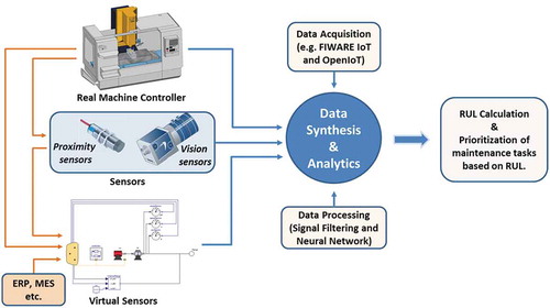
To sum up, PHM exploits the estimation of the machine’s remaining useful life for the identification of the optimal time in order for the next maintenance action to be carried out. The main objective of this research is the calculation of the remaining useful life of each machine in a production plant, based on the combined examination of the machines’ controller data as well as the machines’ physics-based simulation as it is shown in Figure 1.

Figure 1. RUL calculation main concept.

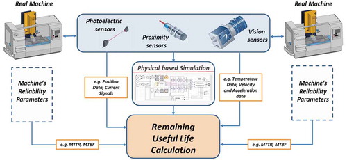
The procedure for addressing this challenge includes four phases:

• The first phase consists of the advanced physical modelling of the machines. Except for the kinematic and dynamic characteristics of the machines, a set of virtual sensors will be integrated into the machines’ simulation models.

• The second phase focuses on the synchronous simulation tuning of the physics-based machine models. As the simulation of the machines’ models is used for their RUL calculation, the machines’ models should be tuned continuously to avoid possible deviations between their real and simulated functionality.

• The third phase consists of the simulation of the physics-based models using as input gathered sensors and machines’ controller data.

• While the fourth phase includes the combining of the simulation outcome and monitored machine data, aiming to predict the machines’ remaining useful life. The reliability parameters of the machines have been integrated into their simulation models. Each phase is described in detail below.

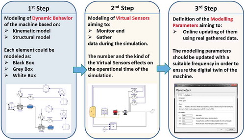
Phase 1: advanced physical modelling of the machines

As depicted in Figure 2, this phase focuses on the advanced physical modelling of the machines. The definition of the kinematic and structural model of the machines takes place initially. The complete model of each machine consists of a number of elements, which represent the dynamic behaviour of each machine’s component based on the modelling of the mechanical, electrical, hydraulic and other functions. In order to have a successful and functional model that can be simulated in an acceptable computational time, it has to be defined which component of each machine should be modelled. Some of the machine’s components are defined as black boxes (without any knowledge of its internal workings) or as grey boxes (using theoretical data to complete its model) or as white boxes, meaning that the exact functionality and the working mechanism of this component are known. Next, the virtual sensors of the model are defined for the completion of the machine’s simulation model. The virtual sensors are modelled as a layout of elements and their functionality is to monitor and gather data from the physics-based models during their simulation. Therefore, it is important to have defined and specified the data to be gathered from the model’s simulation in order to be used in the algorithm of RUL prediction. The use of virtual sensors, at each element and function of the model, increases the computational time of the model’s simulation. Lastly, modelling parameters are defined, which will be used to update the physical model, based on the controller and sensor data. These parameters will be editable and will be associated with the synchronous simulation tuning with the aim to adjust the behaviour of the machine’s model with that of the real machine. More details about the simulation tuning will be described in Phase 2.

Figure 2. Steps of advanced modelling.

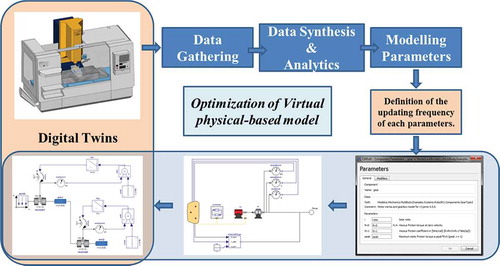
Phase 2: simulation tuning of the physics-based model

This phase focuses on the tuning of the physics-based models, as depicted in Figure 3. The aim of this phase is to realise Digital Twin of the real machines in the simulation environment. The most important step here is the definition of the data that should be monitored both by the machines that are equipped with physical sensors and the controller of the resources. According to Phase 1, the modelling parameters form the base for the definition of these data. A data synthesis technique will also be utilised having taken under consideration both the physical and the computational reductions. As physical reductions, it refers to the amount of data to be synthesised (potential lack of data may occur) while as computational reductions, it refers to the computational time for the data synthesis. The synthesised data target to tuning the models by updating the modelling parameters.

More specifically, the actual data which are gathered by machines’ controller and external sensors will be utilised for two reasons; firstly, to provide them as input in the digital model for the simulation of it and secondly to compare them with the output of the simulation. Accordingly, a comparison between the actual behaviour of the robot and the predicted one will take place. To realise the Digital Twin concept, the modelling parameters which have already defined in Phase 1 aiming to eliminate the error of this comparison should be defined. To achieve it, an estimation of the modelling parameters should take place periodically, and to be provided in the digital model. The tuning procedure is based on the comparison of the actual machine’s component behaviour with the predicted one. Signals are compared in order to perform this comparison. Since the modelling parameters are estimated and the model is tuned, the deviation between the actual and digital machine’s component behaviour is decreased. When this deviation is lower than the desired limit, the tuning procedure stops and the new modelling parameters are obtained and provided to the digital model.

A part of this phase is to define the priority of the online real-time machine’s component tuning. On the one hand, the synchronous tuning of the simulation models will be responsible for keeping the precision of the Digital Twin achievement over 95%, but on the other hand, it is not necessary for all modelling parameters to be continuously updated. Some of the modelling parameters will be tuned with lower frequencies than others because of their lower effect on the simulation process. A weight factor table defines the frequency of tuning for each machine’s component. In this way, the computational time is reduced.

Figure 3. Synchronous simulation tuning mechanism.

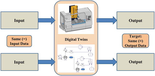
Phase 3: digital twin operation

As depicted in Figure 4, the main objective of this phase is the utilisation of the Digital Twin. After the modelling of the machines (Phase 1) and their tuning during their operation (Phase 2), their simulation is the next step. The same tasks that the real machines have to perform are used as input to the simulation. These tasks are performed virtually by using the simulation software and their outcome is used for the RUL calculation of each machine (Phase 4). The output of the virtually performed tasks is compared with the actual output of the real machine operation. The results of this comparison are used for the RUL calculation.

Figure 4. Simulation of the digital models.

Phase 4: RUL calculation

Here, as it depicted in Figure 5, the components’ RUL is calculated by considering the data gathered from the sensors and the machines’ controllers as well as from the simulation of the machines’ physics-based models. The model's integrated simulation allows for the prediction of the system’s behaviour under different working conditions. Furthermore, the digital models can be used for the simulation of the machines’ in the future based on the defined production plan. The necessity of Digital Twin arises from the fact that the collected sensor data are not always adequate for the RUL estimation. By using physics-based models, you can extrapolate data using virtual sensors based on the mathematical representation of the machine.

The monitored parameters can be related – indicatively – to temperature, voltage, current, torque and power. They are gathered by the machine’s controller directly, whilst the physics-based simulation models use the Virtual Sensors as described in Phase 2. All these measurements are filtered and grouped for a specific time phase. This filtering and grouping are performed in order to avoid capturing random abrupt changes of the parameters which are not important to the machine’s condition. The outcome of this phase allows for the calculation of the machines’ component RUL during their operations.

The RUL prediction is based on the comparison of the predicted behaviour of the machine ‘s components and the nominal behaviour of the machine ’s components. This comparison is based on signal comparison and more specifically with torque signal comparison. The procedure to estimate the RUL for a machine’s component is to simulate the digital model continuously taking under consideration the future operation plan of the real machine as well as the degradation model of the physics phenomena during the time and to compare the simulation output with the nominal output of the machine. Efficient algorithms are used to process and combine the gathered data aiming to provide the generated information to the simulation software. This information is used as input for the simulation and for the tuning of the simulation models.

Figure 5. RUL calculation methodology.

3. System implementation

In this section, the software which was implemented in order to execute the presented approach is described. The modelling procedure was developed in the OMEdit environment, a Modelica connection editor for OpenModelica. OpenModelica is an open-source Modelica-based modelling and simulation environment intended for industrial usage. Modelica is a non-proprietary, object-oriented, equation-based language to conveniently model complex physical systems. This software allows the user to create models that describe the behaviour of real-world systems in two ways. The first way is to use components from free Modelica Standard Library and the second is to create their own components. Combining these components can create large and complex systems. So, no particular variable needs to be solved manually, as the Modelica tool has been created with the aim to solve them automatically (Mattsson, Elmqvist, and Otterc 1998).

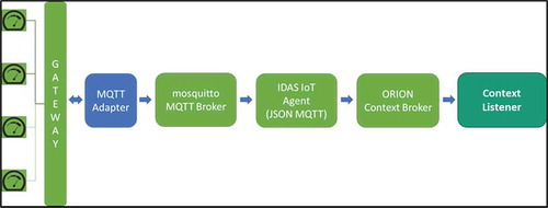
The ‘Data Acquisition’ component is an IoT stack supported by FIWARE components (Steinmetz et al. 2017). The main components are the ORION Context Broker to manage the data context and the IDAS IoT Agent (JSON-MQTT) to mediate between a Message Queuing Telemetry Transport (MQTT) enabled sensor and the context broker. The signal processing methods take place at the gateway level. More specifically, the signals are filtered using an Infinite Impulse Response (IIR) filter to cut undesirable frequencies (noise) (Litwin 2000). The data acquisition and the signal processing method are depicted in Figure 6.

Figure 6. Data acquisition mechanism.

The RUL calculation is based on the output of physics-based simulation in combination with machines’ manufactures data which are used to validate that the calculated RUL is in line with the ideal operation lifetime. Although high deviations may occur during the comparison of this metric, since the RUL is based on the real machines’ operation while manufacturers’ parameters are based on a theoretical level, taking under consideration the nominal operation of a machine and the real-predicted one, the health status of machines’ components can be obtained. Accordingly, the maintenance tasks can be prioritised based on the RUL of each component.

4. Case study

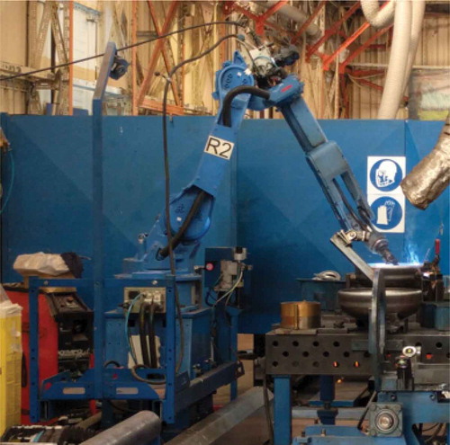
A case study has taken place to demonstrate the functionality of the discussed approach and is presented and discussed here. The resource which was used in the case study was a six-axis robotic structure which is used for welding tasks in the assembly of a thermosiphonic system. Figure 7 depicts the selected resource during its operation.

Figure 7. Real industrial scenario for the system’s validation.

The demonstration of the proposed approach will be presented below per phase in order to be easier the correspondence with the aforementioned information in Approach chapter.

Phase 1: advanced physical modelling of the machines

The digital model of the robot is presented in Figure 8. The modelling level of each digital robot component is presented in Table 1 and arise from the amount of the available data which are used in the modelling. The Mechanical structure component of the robot consisted of the seven links, six joints, six axes, one tool and one base frame which corresponded to the real sub-components of the robot. A number of parameters of each sub-component (e.g. mass, the centre of mass, inertia tensor, axis of each link and others) have been defined partially by the manufacturer of the robot while some of them are extracted from CAD files or estimated using identification procedures. Each axis is utilised as a link between the Mechanical structure component and the six gearbox components. Each gearbox component consists of one ideal gear which represents the gear ratio of each axis, one rotational component with inertia which represents the gears and one bearing which represent the Coulomb friction. Following, each gearbox component is linked with the corresponding input signal component via the actuator component which was responsible to create a torque signal for the motion of the corresponding linked joint based on the input signal component information.

Figure 8. Robot digital model.

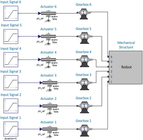
Table 1. Modelling level of each digital component.

Component	Sub-component	Function	Modelling level
Mechanical structure	Link	Represent the rigid bodies of a robot.	White box
	Joint	Represent the rotation of a rigid body around one axis.
	Mass	Represent the tool of the robot at its TCP.
	World frame	Represent the base frame of the robot.
Gearbox	Ideal gear	Represent the gear ratio of the axis.	Grey box
	Bearing friction	Represent the Coulomb friction of the axis.
	Inertia	Represent the mass and the inertia tensors of the gears.
Actuators	–	–	Black box
Input signals	–	–	Black box

As it was described in Approach, the second stage of Phase 1 is the modelling and integration of a number of virtual sensors in the digital model aiming to gather data which are not reached by any other sensorial system or robot’s controller. In this demonstration, three virtual sensors were used aiming to gather the position signal in the output shaft of the gearbox relative to the position signal before the bearing, to gather the speed signal in the output shaft of the gearbox relative to the velocity signal before the bearing and the accelerometer signal in the output shaft of the gearbox relative to the accelerometer signal before the affection of axes’ inertia. The three sensors are integrated into each gearbox of the digital model.

Assuming that the gearbox is the most critical component for the robots’ lifecycle, the modelling parameters of the digital model arise by the gearboxes. More specifically, the parameters which mainly affect the gearboxes’ operation are the modelling parameter Fc which corresponds to the friction component of a robot gearbox and it is relative with the Coulomb friction and the parameter Jm which corresponds to the inertia of the gears (Fernandes et al. 2014). These two parameters will be tuned over the time by a tuning mechanism which is presented in Phase 2.

Phase 2: simulation tuning of the physics-based model

After the modelling phase, the simulation tuning mechanism was implemented to the models aiming to realise the Digital Twin. In this case study, the data which were used for the tuning of the model were data which were gathered from the robot’ controller and accelerometers which were placed on robot’s links. For each gearbox, two signals were monitored; the first one was gathered using the machines’ controller and monitor the actual position signal before the gearbox while the second one was gathered using the accelerometer and monitored the actual torque signal after the gearbox. The same procedure took place continuously and the data were stored in a local database while the simulation was running. For each simulation iteration, the actual position signals for each gearbox were provided as input to the digital model. The inverse dynamic digital model was simulated in OpenModelica and calculate the predicted torque signal for each gearbox. Accordingly, the tuning mechanism requires also the simulation of the model but with the initial values of Fc and Jm as they were defined by gearboxes’ manufacturer.

The data of the real execution and the data of the virtual execution were compared, and the torque errors were calculated. The estimation of the modelling parameters of the model was based on Nonlinear Least Square Method. Using this methodology, the value ranges for parameters were restricted significantly. An iterative process was executed using the estimated parameters with an aim to evaluate behaviourthe of the simulated model. The dynamic parameters for which the calculated errors were minimum were saved for the next execution of the program. This process was executed as many times as the number of the robot experiment having as output an excel file which involved the dynamic parameters of the robot. When the parameters have been estimated successfully, the new values of Fc and Jm were imported in the digital model. Figure 9 presents how the deviation between the actual and the predicted torque signal is eliminated during the tuning of the system by updating the Bm and Jm parameters. These figures are mentioned to Axis 1 of the robot while the same procedure took place for the modelling parameters of other five axes, too.

Figure 9. Torque signal comparison without model tuning (a), during the tuning (b) and after the tuning (c).

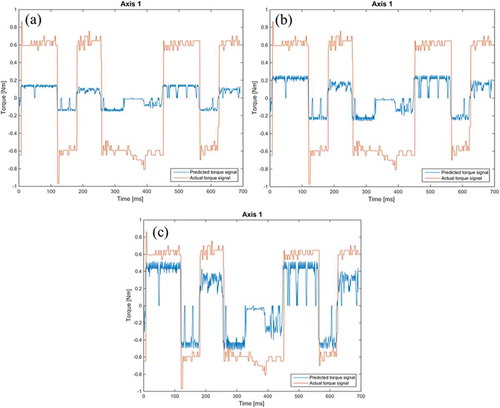
Aiming to reduce the computational time of the system, weight factors are defined for each modelling parameters which underline how often each parameter will be updated. The definition of them was based on the literature and more specific in studies which define how each physical phenomenon affects the machines’ health status (Chandra and Langari 2006; Kang, Zhang, and Jin 2015). The initial time for the execution of a simulation with both parameters to be tuned on each simulation iteration was approx. 260 ms and after the definition of the weight factors, this time period was reduced, by 24%, to 197.6 ms. The tuning weight factor of each modelling parameter is presented in Table 2.

Table 2. Modelling parameters’ tuning weight factors.

Modelling parameters	Tuning weight factor
Fc	80% (update 1 time each 8 simulation cycles)
Jm	60% (update 1 time each 6 simulation cycles)

Phase 3: simulation of the machines’ functionality

After the modelling of the inverse kinematic robot model and the digital model tuning, the simulation of the whole system took place. The monitored position signals of the robot’s motors are converted and imported as input to the simulation via the input signal components. The simulation parameters were defined with aim to execute an accurate and fast simulation. The output of the simulation is the torque signals of each robot ‘s gearbox which occurred in order to move the simulated robot as the real one. The simulation parameters are presented in Table 3.

Table 3. Simulation parameters.

Simulation parameters	Values
Number of intervals	30
Start time	0 s
Stop time	0.6 s
Integration method	Dassl
Jacobian	Coloured Numerical
Tolerance	1e-06

Phase 4: RUL calculation

Since the Digital Twin has been created, the digital models are ready to be used for the simulation of the gearboxes in different operation cases. A set of experiments took place and the health status of each robot gearbox was calculated as a result of the comparison between the nominal function of the robot and the predicted one which was obtained by the digital model. When the difference between them passed a predefined limit, then the RUL calculation algorithm provided the RUL of each element for the corresponding operation case of the machine.

The production plan of the manufacturing company and mainly the tasks of the welding robot were taken under consideration for the execution of the experiments. The figures below depict the operation of Axis 1 gearbox of the robot during its simulation for a six-month time period. The simulation of the robot took place once per day within the defined time period, although one diagram per month is shown to depict how the bearing friction (Fc) and the inertia of the gears (Jm) effect on gearbox health status. In the same way, all the gearboxes of the robot were simulated, and the RUL was estimated.

Figure 10. Nominal torque signal of the Axis 1 gearbox during the execution of the welding task.

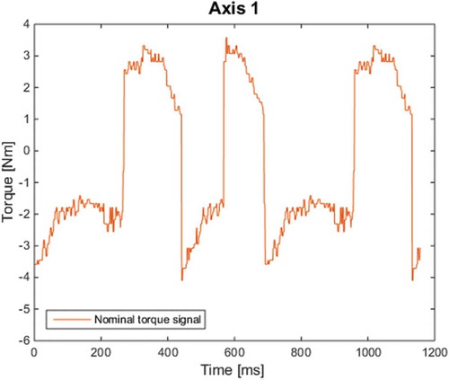
Figure 11. Comparison of predicted and nominal torque signals after 1 month.

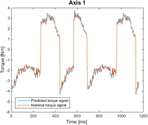
Figure 12. Comparison of predicted and nominal torque signals after 4 months.

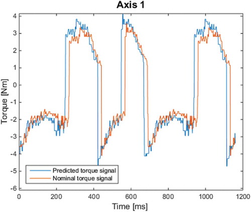
Figure 13. Comparison of predicted and nominal torque signals after 6 months.

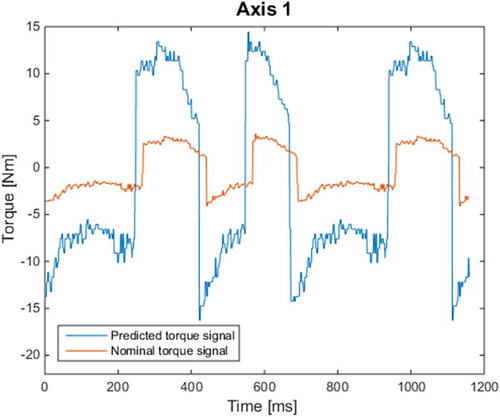
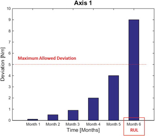
As it is shown in the Figure 10–13, the deviation between the nominal torque signal and the predicted torque signal was increased during the time due to the wear. In Figure 14, the deviations are presented. The maximum allowed deviation was defined by the user of the robot taking under consideration historical data and previous experience.

Figure 14. RUL calculation based on maximum allowed deviation.

5. Discussion

Based on the aforementioned case study, the RUL of robot Axis 1 gearbox was 6 months. It means that the deviation between the nominal torque signals which should be applied to the robot gearbox in order to perform the welding tasks by moving the robot, and the predicted signals which are estimated taking under consideration the future production plan and the degradation profiles of gearbox components, has exceeded the maximum allowed limit. The digital model of each component was updated daily via the tuning of the modelling parameters Fc and Jm. To achieve this, the required data were gathered by the robot’s controller aiming to identify the component behaviour and to adjust the digital models of them accordingly. In a similar way, the other robot gearboxes' RUL was estimated. The same experiment was repeated continuously one time per day – after the tuning of the digital models. So, the simulation iteration for the RUL calculation in this application was once per day. The calculated RUL was the same in all experiments. Small modifications may occur if the calculation takes place in daily base and not in monthly base as in the presented scenario.

Taking under consideration the results of the presented pilot case, the proposed methodology enables the machine’s component RUL prediction and it can be a part of a more generic predictive maintenance framework. Except for the RUL estimation methodology, the proposed methodology focuses also on the creation of digital models and the enabling of the Digital Twin concept. In this research, the method was implemented and validated on the gearboxes of a robot. Although the same procedure can be applied in other components, too.

Finally, a number of limitations and weaknesses have been identified in this research. Firstly, it is assumed that the most critical components of a gearbox are the bearings. According to literature, the main causes of bearing failures are related to loading and lubrication issues. In this research, we are focusing mainly on the wear prediction under normal operating conditions of a gearbox. This means that the loading is in the range given by the manufacturer while the lubrication is deteriorated due to operational time. This is the reason why this paper is focusing on friction. The proposed approach is open in order to integrate vibration parameters in the future, in another case study. Of course, the authors will investigate the gearbox wear due to vibrations in the future. Secondly, the proposed methodology has not been validated through a real scenario which includes a machine’s component breakdown. It means that the methodology works, and the RUL of each component is estimated. Although, a real breakdown will validate that the RUL was estimated with high precision or not. Thirdly, the physics-based models of some components have been modelled as black boxes. It increases the possibilities of a non-precise RUL estimation for these components. Almost all of these limitations will be investigated by the authors in the future.

6. Conclusion and future work

For the scope of the experiment, a defective gearbox of Axis 1 of the robot was used to validate the proposed system. It was demonstrated though that the presented approach utilising Digital Twin to estimate RUL provides accurate results that can be for predictive maintenance considerations and related decision-making, such as for production planning. Accordingly, the presented approach can be applied, and it is mostly used, for manufacturing resources that do not typically have such long RUL.

More specifically, the utilisation of a physics-based simulation model offers a variety of advantages. At first, the condition and the status of the machine can be predicted as a result from the simulation of physics-based models, without the machines’ operation being stopped, as it happens in the common predictive maintenance solutions. The presented RUL calculation method enables the continuous update of information, related to the machines’ condition at component level since it can be executed in a loop and in a very short time. In this way, it is feasible to know the status of each machine for each one of its tasks. In case that a statistical analysis is required to be implemented, this method can be used for data generation since the user can provide as input virtual tasks. Finally, the user is able to know of the way that the machine’s condition will be affected by the execution of a task even before its execution. Consequently, the specific method can be used in order to support the user on assigning specific tasks on the specific manufacturing resources (Chryssolouris et al. 2008a).

As a future activity, the authors plan to integrate the proposed methodology in a more generic predictive maintenance framework which the main role will be the evaluation of the machines’ health status and the planning of the maintenance activities. Furthermore, the authors plan to proceed with a future study that will focus on a more detailed modelling of machine components is aimed, as it will eliminate any possible errors and uncertainties, thus leading to a more accurate RUL calculation. In addition, the tuning weight factors of the modelling parameters will be defined by a set of real-time experiments. In the same way, research will work on the developing of degradation models for the friction and other critical physic phenomena which affect the machines’ health status. Finally, the proposed methodology will be implemented in other kinds of machines and will be validated by monitoring the machine until a real breakdown aiming to evaluate the accuracy of this approach.

Acknowledgments

Part of the work reported in this paper makes reference to the EC research project “PROGRAMS – PROGnostics based Reliability Analysis for Maintenance Scheduling” (www.programs-project.eu), which has received funding from the European Union’s Horizon 2020 research and innovation programme under the Grant Agreement No. 767287.

Disclosure statement

No potential conflict of interest was reported by the authors.

References

- Aivaliotis, P., K. Georgoulias, Z. Arkouli, and S. Makris. 2019. “Methodology for Enabling Digital Twin Using Advanced Physics-based Modelling in Predictive Maintenance.” Procedia CIRP 81: 417–422. doi:10.1016/j.procir.2019.03.072.
- Aivaliotis, P., K. Georgoulias, and G. Chryssolouris 2017. “A RUL Calculation Approach Based on Physical-based Simulation Models for Predictive Maintenance.” International Conference on Engineering Technology and Innovation (ICE IEEE), Portugal, 1243–1246. doi:10.1007/s00784-016-1893-1.
- Baraldi, P., F. Mangili, and E. Zio. 2015. “A Prognostics Approach to Nuclear Component Degradation Modelling Based on Gaussian Process Regression.” Progress in Nuclear Energy 78: 141–154. doi:10.1016/j.pnucene.2014.08.006.
- Bechhoefer, E., and R. Schlanbusch. 2015. “Generalized Prognostics Algorithm Using Kalman Smoother.” IFAC-Papers On Line 48 (21): 97–104. doi:10.1016/j.ifacol.2015.09.511.
- Chandra, M., and R. Langari 2006. “Gearbox Degradation Identification Using Pattern Recognition Techniques.” IEEE International Conference on Fuzzy Systems, Canada, 1520–1526.
- Chryssolouris, G., D. Mavrikios, N. Papakostas, D. Mourtzis, G. Michalos, and K. Georgoulias. 2008a. “Digital Manufacturing: History, Perspectives, and Outlook.” Proceedings of the Institution of Mechanical Engineers Part B: Journal of Engineering Manufacture 222 (5): 451–462.
- Chryssolouris, G., D. Mourtzis, N. Papakostas, Z. Papachatzakis, and S. Xeromerites. 2008b. “Knowledge Management Paradigms in Selected Manufacturing Case Studies.” Methods and Tools for Effective Knowledge Life-Cycle Management 521–532.
- Efthymiou, K., P. Georgakakis, N. Papakostas, and G. Chryssolouris 2011. “On an Engine Health Management System.” 3rd International Conference of the European Aerospace Societies, Italy.
- Efthymiou, K., N. Papakostas, D. Mourtzis, and G. Chryssolouris 2012. “On a Predictive Maintenance Platform for Production Systems.” 45th CIRP Conference on Manufacturing Systems, Athens, 221–226.
- Fernandes, C., P. Marques, R. Martins, and J. Seabra. 2014. “Gearbox Power Loss. Part II: Friction Losses in Gears.” Tribology International 88: 309–316. doi:10.1016/j.triboint.2014.12.004.
- Jay, L., W. Fangji, Z. Wenyu, G. Masoud, L. Linxia, and S. David. 2014. “Prognostics and Health Management Design for Rotary Machinery systems—Reviews Methodology and Applications.” Mechanical Systems and Signal Processing 42: 314–334. doi:10.1016/j.ymssp.2013.06.004.
- Kang, J., X. Zhang, and T. Jin 2015. “Tracking Gearbox Degradation Based on Stable Distribution Parameters: A Case Study.” IEEE Conference on Prognostics and Health Management, USA, 1–6.
- Li, X., Q. Ding, and J. Sun. 2018. “Remaining Useful Life Estimation in Prognostics Using Deep Convolution Neural Networks.” Reliability Engineering & System Safety 172: 1–11. doi:10.1016/j.ress.2017.11.021.
- Litwin, L. 2000. “FIR and IIR Digital Filters.” IEEE Potentials 19 (4): 28–31. doi:10.1109/45.877863.
- Mattsson, S., H. Elmqvist, and M. Otterc. 1998. “Physical System Modelling with Modelica.” Control Engineering Practice 6 (4): 501–510. doi:10.1016/S0967-0661(98)00047-1.
- MyCar Deliverable D2.3.1 – D3.3.1 – D4.3.1 – D5.3.1 – Refinement and Industrial Implementation.
- Papachatzakis, P., N. Papakostas, and G. Chryssolouris 2007. “Condition Based Operational Risk Assessment an Innovative Approach to Improve Fleet and Aircraft Operability: Maintenance Planning.” 1st European Air and Space Conference, Germany, 121–126.
- Shi, H., and J. Zeng. 2016. “Real-time Prediction of Remaining Useful Life and Preventive Opportunistic Maintenance Strategy for Multi-component Systems considering Stochastic Dependence.” Computers & Industrial Engineering 93: 192–204. doi:10.1016/j.cie.2015.12.016.
- Spreafico, C., D. Russo, and C. Rizzi. 2017. “A State-Of-the-art Review of FMEA/FMECA Including Patents.” Computer Science Review 25: 19–28. doi:10.1016/j.cosrev.2017.05.002.
- Steinmetz, C. et al. 2017. “Ontology-driven IoT Code Generation for FIWARE.” 15th International Conference on Industrial Informatics (INDIN), Germany, 38–43.