Risk-based life cycle cost analysis using a two-level multi-objective genetic algorithm

ABSTRACT

The aim of this study has been to develop a two-level multi-objective genetic algorithm (MOGA) to optimize risk-based LCC analysis to find the optimal maintenance replacement time for road tunnel ventilation fans. Level 1 uses a MOGA based on a financial risk model to provide different risk percentages, while level 2 uses a MOGA based on an LCC model to estimate the optimal fan replacement time. Our method is compared with the approach of using a risk-based LCC model. The results are promising, showing that the risk-based LCC offers the possibility of significantly reducing the maintenance costs of the ventilation system by optimising the replacement schedule by considering the risk costs. The risk-based LCC can be used with repairable components, making it applicable, useful and implementable within Swedish Transport Administration (Trafikverket). In this study, MOGA operators have selected the cost of maintenance and risk data through the previous levels using different ways to provide different possible solutions. A drawback of the MOGA based on a risk-based LCC model with regard to its estimation is that a late replacement period over 20-year period might increase the maintenance cost. Therefore, the MOGA does not provide a good solution for a risk-based LCC.

KEYWORDS:

• Life cycle cost (LCC)
• multi-objective genetic algorithm (MOGA)
• risk-based life cycle cost
• optimal maintenance replacement time
• optimization

1. Introduction

The importance of structural maintenance is widely recognized nowadays. To establish a rational maintenance programme, it is important to develop a cost decision-support system for the maintenance of existing infrastructures (Furuta et al. 2004). ‘Life cycle cost’ (LCC) is a useful concept in reducing the overall cost and achieving an appropriate allocation of resources (Frangopol and Furuta 2001). The optimization of the LCC consists of minimizing the expected total cost, which includes the costs for planning, purchase, operation and maintenance (i.e. corrective and preventive maintenance), and liquidation. The cost of corrective maintenance is the cost of the performed action, while the cost of preventive maintenance is the cost of the planned maintenance (Nilsson and Bertling 2007). The optimal strategy obtained by LCC optimization can differ according to the different reliability levels (Furuta et al. 2004).

‘A LCC analysis that does not include risk analysis is incomplete at the best and can be incorrect and misleading at worst’ (Craig 1998). LCC analysis combined with risk analysis provides different decision scenarios and the different consequences of these decisions. Some of these analyses might not be applicable because of different operational and environmental situations (Markeset and Kumar 2001). However, the goal is to estimate and compare the likelihood of success or failure for all the optimizations of the LCC with the different levels of reliability. Reliability can be defined as the probability that the system can perform continuously and without failure over a period of time when operated under stated conditions.

LCC for tunnel fans system is an important case study because 121 fans that needs to be mainly operated for reducing the pollution and getting fresh air within the tunnel. Tunnel fans are designed for ventilation and smoke control in tunnels. The jet fans use the impulse principle to move air through the tunnels in a longitudinal direction. These fans required maintenance and replacement to keep operated. The maintenance cost is high if does not consider on the proper time. In addition, the failure in fans might increase the cost risks and the total risk in the tunnel. Therefore, LCC is necessary to find the optimal replacement time to keep the service of fans.

Traditional LCC calculation methods are able to compare different available solutions that are influenced by various cost parameters (Hinow and Mevissen 2011). A multi-objective genetic algorithm (MOGA) provides the possibility of obtaining several optimal solutions that have different LCC values. In fact, real-world systems are often nonlinear (Hansen, McDonald, and Nelson 1999). The MOGA is often compatible with nonlinear systems and uses a particular optimization from the principle of natural selection of the optimal solution on a wide range of LCC populations (Hatzakis and Wallace 2006).

The GA is a well-established method which helps in solving complex and nonlinear problems that often lead to cases where the search space shows a curvy landscape with numerous local minima. The MOGA is designed to find the best LCC value through an LCC model that is based on the selected cost values to compute the LCC. The calculation of the LCC model is influenced by the cost values that have been selected using the GA operations. In addition, the MOGA can evaluate the model error by comparing different scenarios.

Liu & Frangopol (Liu and Frangopol 2005) formulated the life cycle maintenance planning of deteriorating bridges as a multi-objective optimization problem. These authors used a MOGA as a search engine to locate automatically an optimal maintenance solution that would minimize the LCC for a large pool of different maintenance scenarios. The results of Monte Carlo simulation have shown uncertainties associated with the deterioration and maintenance processes that may have important effects on estimating the life cycle maintenance cost. In addition, the approach of (Liu and Frangopol 2005) might not be efficient for long-term performance estimation.

Elbehairy et al. (Elbehairy et al. 2006) applied GAs and a shuffled frog leaping algorithm to an LCC model of bridge deck repairs to optimize maintenance and repair decisions. Ten trial runs with different numbers of bridges were experimented with to evaluate the performance of both types of algorithms. The algorithms proposed by these authors show a stable handling of their research problem. The benefits of the bridge deck management system are illustrated along with various strategies to improve the optimization performance. However, the issue is to determine the set of parameters that optimize the performance and improve the total performance.

Caputo et al. (Caputo, Pelagagge, and Palumbo 2011) presented a computer-aided methodology for the economic optimization of industrial plant safety. Their methodology is implemented by resorting to a GA to minimize the total safety-related cost, the operating expenses of the adopted safety measures, and the expected monetary loss from accidents. The authors’ model is deterministic, which can be considered as a limitation given the fact that determination of the costs and accident probabilities is difficult. In addition, the economic scenario parameters, such as the discount rate, capital recovery factor and equipment life, are also of a stochastic nature. Accordingly, the authors’ model needs to be extended in the framework of a stochastic optimization problem.

Nývlt et al. (Nývlt, Prívara, and Ferkl 2011) introduced the concept of risk analysis in the field of risk management and employs popular methods in aeronautics and aircraft industry. These authors proposed probabilistic risk assessment (PRA) to enable the minimization of building and refurbishing costs to preserve a satisfactory safety level. Their proposed analysis method was able to cut off almost 67% of the originally calculated costs. The advantage of the method developed by Nývlt et al. (Nývlt, Prívara, and Ferkl 2011) is the accurateness of the results and the method’s suitability for data with a high level of uncertainty; any lack of relevant statistical data is taken into account. The drawback is the ‘free’ structure of the method, which means that it is a framework rather than a guideline and each application has to be treated very carefully.

The aim of the present study has been to develop a two-level MOGA (MOGA) to optimize risk-based LCC analysis in order to find the optimal maintenance replacement time for fans used in road tunnels. Level 1 uses a MOGA based on a financial risk model to provide different risk percentages, while level 2 uses a MOGA based on an LCC model to estimate the optimal replacement time for the ventilation system. Level 1 of the MOGA was applied to the risk cost data for four populations to provide variant probabilities of risk percentages for 15 generations. Level 2 of the MOGA was applied to the cost data objects and the different generations of risk cost data of the first level for four populations to estimate the optimal replacement time. Our method is compared with the approach of using a risk-based LCC analysis model. Risk-based LCC model has combined the financial risk as an important input with LCC model inputs.

2. Data collection

The cost data concern tunnel fans installed in Stockholm in Sweden. The data had been collected over ten years from 2005 to 2015 by Swedish Transport Administration (Trafikverket) and were stored in the MAXIMO computerized maintenance management system (CMMS). In this CMMS, the cost data are recorded based on calendar time for the maintenance of the tunnel fans. Every work order contains corrective maintenance data, a component description, the reporting date, a problem description, and a description of the actions performed. Also included are the repair time used and the labour, material and tool cost of each work order.

In this study, we considered the two cost objects of labour and materials based on the work order input into the CMMS for the ten-year period mentioned above. The tool cost data were not selected because 97% of those data were missing and they could not be used for forecasting. The selected data were clustered, filtered and imputed for the present study using a MOGA based on a fuzzy c-means algorithm (Aldouri, Al-Chalabi, and Zhang 2018). This stage is used to evaluate the data and fix the problems within each cost parameter. MOGA provides the possibility to cluster the data into proper parts and isolate the data problems for fixing the missing and outliers problems.

However, the current data is only for ten years and we need to forecast the data for 30 years for better LCC optimizing. Data forecasting was performed using a MOGA based on the autoregressive integrated moving average (ARIMA). MOGA offers a huge possibility for accurate forecasting and evaluates forecasting using different models (Al-Douri, Hamodi, and Lundberg 2018). It is important to mention that all the cost data used in this study concern real costs without any adjustment for inflation. Due to company regulations, all the cost data have been encoded and are expressed as currency units (cu).

The operating cost data of the fans were generated for each month, based on the energy price, the fans’ working hours, and the fans’ power. Table 1 gives a sample of the generated operating cost data from April 2005 to December 2015. The data were generated based on information from experts at Trafikverket involved in this study. The information which they provided is the following (Al-Chalabi 2018):

• fans’ power: 25–80 kW,

• fans’ operating time per day: 6–8 hours,

• fixed energy price: 2.88 Swedish crowns (SEK)/kWh.

Table 1. Sample of generated operating cost (OC) data (Al-Chalabi 2018)

Fan number	Fan’s power (kW)	Working hours (h)	Energy price (SEK/kWh)	Operating cost/fan.day (SEK)
1	70	7.9	2.88	1593
2	75	6	2.88	1295
3	32	7.5	2.88	695
4	75	7.6	2.88	1654
5	60	7.7	2.88	1332
6	30	6.2	2.88	539
7	40	6.8	2.88	790
8	55	6.52	2.88	1034
9	78	7.56	2.88	1700
No. of days	OC/day (SEK)	Months-year	No. of months	OC/month (SEK)
1	128621	Apr-05	1	3856485
2	129322	Maj-05	2	3931435
3	129725	Jun-05	3	3855434
4	120832	Jul-05	4	3793487
5	132193	Aug-05	5	3870663
6	134786	Sep-05	6	3846868
7	122774	Okt-05	7	3828002
8	131767	Nov-05	8	3839732
9	13307	Dec-05	9	3822851

The failure data used in this study were collected for the ten-year period in question using the CMMS as the source of those data. In the CMMS, the failure data are recorded based on the calendar time of the work order. The time to failure (TTF) was estimated based on the reporting times for corrective maintenance stated in the work orders. The labour and material costs considered were those reported for each work order for corrective maintenance. Failure cost data were forecasted for 20 and 30 years using a MOGA based on the ARIMA model (Al-Douri, Hamodi, and Lundberg 2018).

3. Risk-based life cycle cost (LCC) model

In the present study, it was tested and validated the failure data, testing them for trends using the Laplace trend test and for serial correlation (Ansell & Phillips, 1994). When these tests are used, depending on the results, the classical statistical techniques for reliability modelling may be an appropriate approach (Ascher 2008; Ghosh and Majumdar 2011; Modarres 2016). The Kolmogorov–Smirnov (K-S) test is traditionally used for the selection and validation of probability distribution models (Louit, Pascual, and Jardine 2009). For the reliability modelling of repairable systems, the basic methodology involves analysing the failure data and identifying the failure data with significant consequences. The TTF data are tested concerning the assumption that they are independent and identically distributed (iid). If the assumption that the data are iid is not valid, then classical statistical techniques for reliability analysis may not be appropriate. Therefore, a non-stationary model such as the non-homogeneous Poisson process (NHPP) must be fitted. The proportionality constant of the NHPP is assumed to be uncertain due to the lack of knowledge about the true expected number of defects initiation (Barabady and Kumar 2008; Kuniewski, van der Weide, and van Noortwijk 2009).

Since maintenance cost limitations invariably exist, risk assessment needs to be integrated in the LCC to create a useful and complementary decision making tool (Stewart 2001). Risk assessment clearly defines the reliability and provides a measure of the cost-effectiveness, since reliability is the probability of failures that will necessitate maintenance. The initial stage of risk assessment is to estimate the reliability through fitting the proper distribution. Note that reliability is not simply the probability of failure. The risk of failure or damage entails direct repair and maintenance costs. The risk of disruption of functional use is very real and, therefore, one must aim to eliminate this risk as much as is practicable, but the risk of failure also causes problems and these problems entail costs. However, a more meaningful risk assessment measure is the expected cost of failure, defined in Equation (1)(1) $E_{c_t}={\sum }_{i=1}^M{R}_{f_i}{C}_{f_i}$(1) (Furuta et al. 2004; Stewart 2001).

(1) $E_{c_t}={\sum }_{i=1}^M{R}_{f_i}{C}_{f_i}$(1)

where $E_{c_t}$ is the expected risk cost over $t$ monthly time scale $\left\{0,\dots ,t\right\}$, $R_{f_i}$ is the failure monthly rate, which is the rate of the interval times of two regular repairable failures. $C_{f_i}$ is the failure cost (labour and material cost) associated with the occurrence of each limit over the number of failures $M$. The risk costs were forecasted using a GA based on the ARIMA model for 20 years. The failure rate was increased manually stepwise by 1% to be in total a value ranging from 1% to 250% risk to study the variation of the risk percentage and the association with the LCC. The stepwise by 1% is modifying the original failure rate values through multiplying with the required risk percentage over the original risk percentage then multiple the result failure rate with the cost. Then, the risk cost integrated in the optimization model was used to find the minimum cost against the system benefits.

Since the optimal value of the costs is required to obtain the optimal replacement time (ORT), the following optimization model was developed to find the replacement time (RT) that minimizes the total cost value ($T{C}_{value}$), as shown in the Equations below. The term ‘total cost value’ is defined as the summation of the fan’s purchase price (PP), operating cost (OC), maintenance cost (MC) and resale value $S_t$ over a long period, with replacements occurring at intervals of n periods (Al-Chalabi et al. 2014; Eschenbach 2003).

(2) $MC=CM+PM$(2)

(3) $CM=S{P}_c+L{C}_c$(3)

(4) $PM=S{P}_p+L{C}_p$(4)

(5) $S_t=B{V}_1\times {\left(1-D_r\right)}^{t}t=1,2,3,\dots ,240(months)$(5)

where the following notation is used:

MC: maintenance cost (cu)

CM: corrective maintenance cost (cu)

PM: preventive maintenance cost (cu)

$S{P}_c$: material cost for corrective maintenance (cu)

$L{C}_c$: labour cost for corrective maintenance (cu)

$S{P}_p$: material cost for preventive maintenance (cu)

$L{C}_p$: labour cost for preventive maintenance (cu)

$S_t$: resale value (cu)

BV₁: booking value on first day of operation (cu)

Dr: depreciation rate

t: fan’s lifetime (months).

The depreciation rate, which allows for full depreciation by the end of the planned lifetime of the fan, is modelled by Equation (6)(6) $D_r=1-{\left(\frac{SV}{B{V}_1}\right)}^{\frac{1}{T}}$(6) (Al-Chalabi et al. 2014; Luderer, Nollau, and Vetters 2009).

(6) $D_r=1-{\left(\frac{SV}{B{V}_1}\right)}^{\frac{1}{T}}$(6)

where SV is the scrap value (cu) and $T$ represents the planned lifetime of the fans, which was 240 months in the case study. The fans were assumed to reach their scrap value after ten years.

The next step is to calculate the total ownership cost over each operating month. In this study, the optimal lifetime of the ventilation system was defined as the fan age that minimizes the fan’s total ownership cost. The total ownership cost (TOC) over the period t is denoted by $TO{C}_t,t=1,2,3,\dots ,n$, where $n$ is the number of operating months. By definition,

(7) $TO{C}_t=PP+\left[{\sum }_{t=1}^{RT}\left(M{C}_t+O{C}_t\right)\right]-S\left(t\right),$(7)

where PP is the purchase price (cu) and $M{C}_t$ and $O{C}_t$ are the maintenance and operating costs for the $t$ months, respectively. The reason for using the total ownership cost is to determine the optimal replacement time that minimizes the total ownership cost over the fan’s planned time horizon. We assume that the replacement fans have the same performance and cost as the existing fans (i.e. identical system). The number of replacement cycles during the planned time horizon is modelled as

(8) $M=\left[\frac{Plannedlifetime}{Replacemnttime}\right]=\left[\frac{T}{RT}\right]$(8)

The optimal replacement time is the value of RT that minimizes the total ownership cost value, as shown in Equation (9)(9) $TO{C}_{value}=\left[PP+{\sum }_{t=1}^{RT}(M{C}_t+O{C}_t+E_{c_t})-S_t\right]\times \frac{M}{{\left(1+r\right)}^{\frac{t}{12}}}$(9) (Al-Chalabi et al. 2014).

(9) $TO{C}_{value}=\left[PP+{\sum }_{t=1}^{RT}(M{C}_t+O{C}_t+E_{c_t})-S_t\right]\times \frac{M}{{\left(1+r\right)}^{\frac{t}{12}}}$(9)

where the following notation is used:

$TO{C}_{value}$: total ownership cost value (cu)

RT: replacement time (months) {1, …, t}

$r$: interest rate

M: number of fan replacements.

4. Two-level system of multi-objective genetic algorithms

In this study, a two-level MOGA has been developed, as shown in Figure 1. The GA consists of the following: (1) a MOGA based on a risk model to provide a variation of risk percentages and (2) a MOGA based on an LCC model to estimate the optimal replacement time for tunnel fans. Both levels were applied on forecasted cost data and risk cost data for 20 years. Level 1 of the MOGA was applied to the risk cost data for four populations to provide variant probabilities of risk percentages for 15 generations. Level 2 of the MOGA was applied to the cost data objects (i.e. the maintenance cost, initial cost, operation cost, and second-hand value) and the different generations of risk cost data of the first level for four populations to estimate the optimal replacement time. The first and second levels use a cross-validation technique to validate the optimization and estimate the system accurateness. Using two levels allows us to reduce the computational cost (Thomassey and Happiette 2007), while reaching an effective and reasonable solution (Ding, Cheng, and He 2007).

Figure 1. Two-level system of MOGAs

4.1. Level one: MOGA based on a risk model

The proposed MOGA method uses a particular optimization from the principle of natural selection of the optimal solution on a wide range of forecasting populations. The MOGA creates populations of chromosomes as possible answers to estimate the optimum forecasting (Hatzakis and Wallace 2006). In the literature, it is reported that the GA is robust, generic and easily adaptable because it can be broken down into the following steps: initialization, evaluation, selection, crossover, mutation, update and completion. The evaluation (fitness function) creates the basis for a new population of chromosomes. The new population is formed using specific genetic operators, such as crossover and mutation (Cordón et al. 2001; Shi et al. 2013). The fitness function is derived from a risk cost estimation model.

The MOGA is a technique that can be used to provide variant probabilities of cost risk percentages for 15 generations. Fifteen generations are enough for these data because the curves of the fitness functions are repeated after fifteen generations. The GA provides non-linear solutions to complex non-linear problems that often lead to cases where the search space shows curvy local minima. In addition, the GA offers the possibility of obtaining solutions that have different reliability levels. The first level utilises a MOGA based on a risk model. The process is as follows: a random number of failure cost data are selected based on encoding in each of the four implementations, and the modified random cost data are generated 15 times. The following steps explain the use of the MOGA for risk cost data.

Step 1: Initial population

A longitudinal study of the risk cost object ($Z^{risk}$) is used to provide the risk percentage variation using the MOGA.

Step 2: First GA generation and selection

The first generation is performed by randomly selecting 80% of the risk objects to ensure that the model includes all the possible patterns up to the edge of the modelling domain.

Step 3: Encoding

Random values, either ones or zeros, are generated for each selected cost data object. Encoding is the process of transforming from the phenotype to the genotype space before proceeding with MOGA operators and finding the local optima.

Step 4: Fitness function

The risk of failure or damage entails direct repair and maintenance costs. The fitness function is based on the risk model in Equation (1)(1) $E_{c_t}={\sum }_{i=1}^M{R}_{f_i}{C}_{f_i}$(1) .

Step 5: Crossover and mutation

In this study, a one-point crossover with a fixed crossover probability has been used. This probability decreases the bias of the results over different generations caused by the huge data values. For chromosomes of length $l$, a crossover point is generated in the range [1, 1/2 $l$] and [1/2 $l$, $l$]. The values of objects are connected and should be exchanged to produce two new offspring. We select two points to create more value ranges and find the best fit.

Randomly ten percent of the selected chromosomes undergo mutation with the arrival of new chromosomes. For the risk cost object values, we swap two opposite data values. The purpose of this small mutation percentage is to keep the risk average changes steady over different generations.

Step 6: New generation

The new generation repeats steps 3 to 5 continuously for 15 generations. The selected fifteen generations are used individually for the second level to validate the forecasting accuracy for each object and population. This step yields fully correlated data for the next step.

4.2. Level two: MOGA based on an LCC model

In this level, MOGA based on an LCC model is implemented as an optimization technique that can be used to estimate an accurate LCC model to find the optimal replacement time. This MOGA is implemented four different times using a cross-validation randomization technique. The process is as follows: a random number of cost data are selected based on encoding in each of the four implementations and the modified random cost data are generated 15 times. Fifteen generations are enough for these data because the curves of the fitness functions are repeated after fifteen generations. The modifications are used to find the optimal forecasting cost data. The following steps explain the use of the MOGA.

Step 1: Initial population

A longitudinal study of each cost object ($Z^{risk},Z^{MC}$, $Z^{OC}$, $Z^{PP}$, $Z^{SH}$) is used to optimize the LCC using the MOGA.

Step 2: First GA generation and selection

The first generation is performed by randomly selecting 80% of the cost objects to ensure that the model includes all the possible patterns up to the edge of the modelling domain. The selected data are used to calculate the fan’s maintenance cost (MC), operation cost (OC), purchase price (PP), and second-hand value (SH).

Step 3: Encoding

Random values, either ones or zeros, are generated for each selected cost data object. Encoding is the process of transforming from the phenotype to the genotype space before proceeding with MOGA operators and finding the local optima.

Step 4: Fitness function

The fitness function is based on the ORT model for time series forecasting of cost data objects individually as seen in Equation (9)(9) $TO{C}_{value}=\left[PP+{\sum }_{t=1}^{RT}(M{C}_t+O{C}_t+E_{c_t})-S_t\right]\times \frac{M}{{\left(1+r\right)}^{\frac{t}{12}}}$(9) .

The fifth and sixth step of the MOGA are described in the section above dealing with the first level.

5. Results and discussions

5.1. Risk-based LCC model results

The reliability assessment of the collected data for the repairable ventilation system led to a better understanding of the failure patterns that influenced the decision-making process concerning the planning of the maintenance activities of the plant. The validation of the assumption that the data were independent and identically distributed (iid) showed a trend in the failure data. The NHPP had to be fitted because the classical statistical techniques of reliability analysis were not appropriate in our case study. Then, the expected ROCOF (rate of occurrence of failures) was used as an intensity function to estimate the failure rate of the TTF data. For repairable systems, the failure rate estimated using the ROCOF shows variant values over time. This rate was used to estimate the risk cost over time.

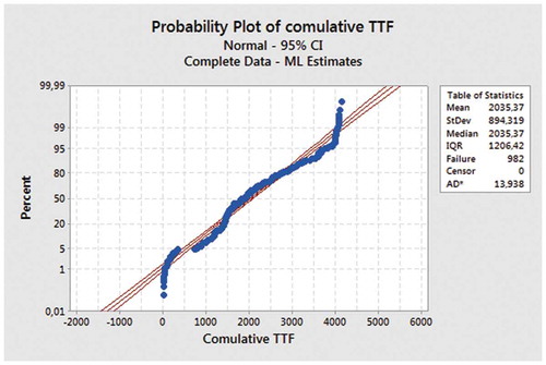
To approximate a large variety of distributions in large data samples, the normal distribution is fitted on accumulated TTF data. Figure 2 shows the fitting estimation of the normal distribution on the TTF data with some statistical results. The normal distribution can give the shape of the reliability against the failure rate of the repairable system over a ten-year time scale.

Figure 2. Normal distribution of cumulative TTF

Figure 3 shows the estimation of the risk costs without accumulative and illustrates that they increased over the period from month 30 to 50. The risk costs increased during this period due to the total fan replacement, which required labour and fan replacement costs. The fail description of the highest peak that one of the fans has an electricity problem, which required to be replaced. After this period, the risk costs decreased steadily because the system is repairable and Trafikverket provided better maintenance and service since they understood the system better.

Figure 3. Risk cost estimation

The LCC optimization was tested for different risk percentages from 1% to 250%. The risk percentage affects the risk cost calculation and then the LCC optimization. The relation between the risk and the LCC is exponential. Figure 4 shows the LCC optimization including a risk of 2% and gives the minimum cost for this risk percentage. The minimum $TO{C}_{value}$ achieved in practice was between month 97 and 117. In our terminology, this replacement time range can be termed the optimal replacement time range. Finding the optimal replacement time range is an important result of our study as it can help users (in this case Trafikverket) in their planning. Trafikverket has the flexibility of being able to make replacements within an optimal replacement time range of 20 months.

There is no fixed date or age within the proposed minimum $TO{C}_{value}$ range at which the total cost is at a minimum, but a decision to replace the system before or after this optimal replacement time range will incur greater costs. The use of a lower replacement age (i.e. less than 97 months) will incur higher costs because of the high investment cost. Meanwhile, if the lifetime of the system exceeds the upper limit of the proposed TOC range, the losses will increase for the following two reasons.

• The cost of operation and maintenance increases when the operating time increases because of fan degradation.

• A fan’s resale value will decrease each month of operation until it reaches its scrap value at the end of its planned lifetime (i.e. 240 months).

Figure 4. ORT of 121 fans as one system with a 2% risk cost

Figure 5 shows the LCC optimization including a risk of 250% and illustrates how increasing risk percentages affect the LCC optimization. The minimum $TO{C}_{value}$ achieved in practice was between month 110 and 130, which still gives an optimal replacement time range of 20 months. The $TO{C}_{value}$ trend shows a different behaviour from that shown in Figure 4, especially over the period lasting from month 25–35. In this case, the LCC optimization does not reflect the proper replacement time range. In addition, Figure 5 shows the significance of risk analysis for the LCC optimization and how an erroneous estimation of the optimal replacement time can lead to an improper maintenance decision.

Figure 5. ORT of 121 fans as one system with a 250% risk cost

LCC analysis without risk analysis might lead to improper decisions due to a lack of knowledge of the failure consequences. Therefore, risk analysis should be an integral part of estimating the LCC.

5.2. Results of the two-level system of MOGAs

5.2.1. Results for level 1: MOGA based on risk cost analysis

In this part of the study, it was tested four populations individually using the MOGA based on the risk model to provide, for the next level, a variation of risk cost percentages based on the TTF data without any external effect (i.e. by adding 1% to the values to change the percentage). The risk cost percentages for each population obtained with 15 different generations were then used as an input for each generation at the next level. Figure 6 shows the minimum risk cost for the four populations over the different generations. The minimum risk cost is given for the different populations taken together. The period between month 11 and 31 shows high-risk costs, which is reasonable due to the maintenance effort required during this time. After month 31, the risk cost over the selected months decreases steadily until month 61, as shown in Figure 6. In month 61, the failure cost is increased due to a replacement, after which the operation is stable for the remaining time.

Figure 6. Risk cost analysis of 121 fans as one system

5.2.2. Results for level 2: MOGA based on an LCC model

The outcome from the first level, specifically for each generation for each population, indicates the LCC optimization for each cost and risk object. For each generation, the MOGA based on an LCC model with a risk analysis model was used to find the minimum maintenance cost through 15 different generations. These generations over different populations offer the possibility of finding an accurate LCC optimization through comparing the behaviour of the different models and revealing which optimal replacement period is appropriate. For different populations, there are different optimizations of the LCC for the different risk costs.

The data selected by the GA operators for calculating the LCC optimization affect the $TO{C}_{value}$. Figure 7 shows the best and minimum $TO{C}_{value}$ of the selected period of time over different variant populations and generations. The minimum $TO{C}_{value}$ that could be achieved in practice was between month 201 and 221 and was found in the second generation. In this case, the GA operators had selected and operated the cost of maintenance and risk data through the previous levels 1 and 2 using different ways to provide different possible solutions. These possible solutions have different variations in the cost values. The variation of the $TO{C}_{value}$ in Figure 7 is extremely increased compared with that of the previous $TO{C}_{value}$. This result exposes a drawback in the estimation using the GA, namely that a late replacement period over a 20-year period might increase the maintenance cost.

Figure 7. ORT of 121 fans as one system for the optimal result

Figure 8 shows the trend of the $TO{C}_{value}$ for the fourth population and, specifically, for the fifth generation, and the $TO{C}_{value}$ here are very high compared with those shown in Figure 7. In Figure 8 one can observe that the minimum $TO{C}_{value}$ that could be achieved in practice was between month 109 and 130 and was found in the second generation. The advantage of using different populations with different selected data is that thereby one obtains a better understanding of the optimal replacement time and can make reliable maintenance decisions.

Figure 8. Example of worst ORT of 121 fans as one system

The results of the two-level system of MOGAs do not show that risk cost analysis plays a significant role in LCC analysis. The MOGA does not help our model, even with wide variances, in optimizing the LCC of the ventilation system. The expected replacement estimation has a bias in the cost values and ORT, which would not lead to proper and efficient maintenance decisions.

6. Conclusions

In this study, it has been concluded that the MOGA model based on a risk-based LCC model has drawbacks when used to estimate the optimal replacement time for the fans of the ventilation system. The results have revealed uncertainties associated with estimating the optimal replacement time which may have significant effects on estimating the system performance profiles and the life cycle maintenance cost.

However, the MOGA model does not achieve a better estimation of the optimal replacement time, while risk-based LCC analysis provides a reasonable estimation of that time. In addition, LCC analysis combined with risk analysis leads to proper maintenance decisions due to increased knowledge of the failure consequences. Therefore, risk analysis should be performed as an integral part of calculating the LCC.

Disclosure statement

No potential conflict of interest was reported by the authors.

References

- Al-Chalabi, H. 2018. “Life Cycle Cost Analysis of the Ventilation System in Stockholm’s Road Tunnels.” Journal of Quality in Maintenance Engineering 24 (3): 358–375. (just-accepted), 00-00. doi: 10.1108/JQME-05-2017-0032.
- Al-Chalabi, H., F. Ahmadzadeh, J. Lundberg, and B. Ghodrati. 2014. “Economic Lifetime Prediction of a Mining Drilling Machine Using an Artificial Neural Network.” International Journal of Mining, Reclamation and Environment 28 (5): 311–322. doi:10.1080/17480930.2014.942519.
- Al-Douri, Y., H. Hamodi, and J. Lundberg. 2018. “Time Series Forecasting Using A Two-level Multi-objective Genetic Algorithm: A Case Study of Cost Data for Tunnel Fans.” Algorithms 11 (8): 123. doi:10.3390/a11080123.
- Aldouri, Y. K., H. Al-Chalabi, and L. Zhang. 2018. “Data Clustering and Imputing Using A Two-level Multi-objective Genetic Algorithm (GA): A Case Study of Maintenance Cost Data for Tunnel Fans.” Cogent Engineering 5 (1): 1–16. doi:10.1080/23311916.2018.1513304.
- Ansell, J. I., and M. J. Phillips. 1994. Practical Methods for Reliability Data Analysis (No. 14). Oxford University Press.
- Ascher, H. E. 2008. “Repairable Systems Reliability.” Encyclopedia of Statistical Sciences, 4.
- Barabady, J., and U. Kumar. 2008. “Reliability Analysis of Mining Equipment: A Case Study of A Crushing Plant at Jajarm Bauxite Mine in Iran.” Reliability Engineering & System Safety 93 (4): 647–653. doi:10.1016/j.ress.2007.10.006.
- Caputo, A. C., P. M. Pelagagge, and M. Palumbo. 2011. “Economic Optimization of Industrial Safety Measures Using Genetic Algorithms.” Journal of Loss Prevention in the Process Industries 24 (5): 541–551. doi:10.1016/j.jlp.2011.01.001.
- Cordón, O., F. Herrera, F. Gomide, F. Hoffmann, and L. Magdalena. 2001.“Ten Years of Genetic Fuzzy Systems: Current Framework and New Trends.” In IEEE Proceedings joint 9th IFSA world congress and 20th NAFIPS international conference (Cat. No. 01TH8569), Vol. 3, 1241–1246. Canada.
- Craig, B. 1998. “Quantifying the Consequence of Risk in Life Cycle Cost Analysis.” Paper presented at the Proceedings of the First International Oil & Gas Industry Forum on Life Cycle Cost, Stavanger, 28–29.
- Ding, C., Y. Cheng, and M. He. 2007. “Two-level Genetic Algorithm for Clustered Traveling Salesman Problem with Application in Large-scale TSPs.” Tsinghua Science and Technology 12 (4): 459–465. doi:10.1016/S1007-0214(07)70068-8.
- Elbehairy, H., E. Elbeltagi, T. Hegazy, and K. Soudki. 2006. “Comparison of Two Evolutionary Algorithms for Optimization of Bridge Deck Repairs.” Computer‐Aided Civil and Infrastructure Engineering 21 (8): 561–572. doi:10.1111/j.1467-8667.2006.00458.x.
- Eschenbach, T. 2003. Engineering Economy: Applying Theory to Practice. New York: Oxford University Press.
- Frangopol, D. M., and H. Furuta. 2001. Life-cycle Cost Analysis and Design of Civil Infrastructure Systems. American Society of Civil Engineers.
- Furuta, H., T. Kameda, Y. Fukuda, and D. M. Frangopol. 2004. “Life-cycle Cost Analysis for Infrastructure Systems: Life-cycle Cost Vs. Safety Level Vs. Service Life.” In Life-cycle Performance of Deteriorating Structures: Assessment, Design and Management, 19–25.
- Ghosh, S., and S. K. Majumdar. 2011. “Reliability Modeling and Prediction Using Classical and Bayesian Approach: A Case Study.” International Journal of Quality & Reliability Management 28 (5): 556–586. doi:10.1108/02656711111132580.
- Hansen, J. V., J. B. McDonald, and R. D. Nelson. 1999. “Time Series Prediction with Genetic‐Algorithm Designed Neural Networks: An Empirical Comparison with Modern Statistical Models.” Computational Intelligence 15 (3): 171–184. doi:10.1111/0824-7935.00090.
- Hatzakis, I., and D. Wallace. 2006. “Dynamic Multi-objective Optimization with Evolutionary Algorithms: A Forward-looking Approach.” In Proceedings of the 8th Annual Conference on Genetic and Evolutionary Computation, 1201–1208, USA.
- Hinow, M., and M. Mevissen. 2011. “Substation Maintenance Strategy Adaptation for Life-cycle Cost Reduction Using Genetic Algorithm.” IEEE Transactions on Power Delivery 26 (1): 197–204. doi:10.1109/TPWRD.2010.2065247.
- Kuniewski, S. P., J. A. M. van der Weide, and J. M. van Noortwijk. 2009. “Sampling Inspection for the Evaluation of Time-dependent Reliability of Deteriorating Systems under Imperfect Defect Detection.” Reliability Engineering & System Safety 94 (9): 1480–1490. doi:10.1016/j.ress.2008.11.013.
- Liu, M., and D. M. Frangopol. 2005. “Multiobjective Maintenance Planning Optimization for Deteriorating Bridges considering Condition, Safety, and Life-cycle Cost.” Journal of Structural Engineering 131 (5): 833–842. doi:10.1061/(ASCE)0733-9445(2005)131:5(833).
- Louit, D. M., R. Pascual, and A. K. Jardine. 2009. “A Practical Procedure for the Selection of Time-to-failure Models Based on the Assessment of Trends in Maintenance Data.” Reliability Engineering & System Safety 94 (10): 1618–1628. doi:10.1016/j.ress.2009.04.001.
- Luderer, B., V. Nollau, and K. Vetters. 2009. Mathematical Formulas for Economists. Springer Science & Business Media, Germany.
- Markeset, T., and U. Kumar 2001. “R&M and Risk-analysis Tools in Product Design, to Reduce Life-cycle Cost and Improve Attractiveness.” Paper presented at the Reliability and Maintainability Symposium, 2001. Proceedings, USA. Annual, 116–122.
- Modarres, M. 2016. Risk Analysis in Engineering: Techniques, Tools, and Trends. USA: CRC press.
- Nilsson, J., and L. Bertling. 2007. “Maintenance Management of Wind Power Systems Using Condition Monitoring Systems—life Cycle Cost Analysis for Two Case Studies.” IEEE Transactions on Energy Conversion 22 (1): 223–229. doi:10.1109/TEC.2006.889623.
- Nývlt, O., S. Prívara, and L. Ferkl. 2011. “Probabilistic Risk Assessment of Highway Tunnels.” Tunnelling and Underground Space Technology 26 (1): 71–82. doi:10.1016/j.tust.2010.06.010.
- Shi, C., Y. Cai, D. Fu, Y. Dong, and B. Wu. 2013. “A Link Clustering Based Overlapping Community Detection Algorithm.” Data & Knowledge Engineering 87: 394–404. doi:10.1016/j.datak.2013.05.004.
- Stewart, M. G. 2001. “Reliability-based Assessment of Ageing Bridges Using Risk Ranking and Life Cycle Cost Decision Analyses.” Reliability Engineering & System Safety 74 (3): 263–273. doi:10.1016/S0951-8320(01)00079-5.
- Thomassey, S., and M. Happiette. 2007. “A Neural Clustering and Classification System for Sales Forecasting of New Apparel Items.” Applied Soft Computing 7 (4): 1177–1187. doi:10.1016/j.asoc.2006.01.005.