Structural production layer decomposition: a new method to measure differences between MRIO databases for footprint assessments

ABSTRACT

Recent empirical assessments revealed that footprint indicators calculated with various multi-regional input–output (MRIO) databases deliver deviating results. In this paper, we propose a new method, called structural production layer decomposition (SPLD), which complements existing structural decomposition approaches. SPLD enables differentiating between effects stemming from specific parts in the technology matrix, e.g. trade blocks vs. domestic blocks, while still allowing to link the various effects to the total region footprint. Using the carbon footprint of the EU-28 in 2011 as an example, we analyse the differences between EXIOBASE, Eora, GTAP and WIOD. Identical environmental data are used across all MRIO databases. In all model comparisons, variations in domestic blocks have a more significant impact on the carbon footprint than variations in trade blocks. The results provide a wealth of information for MRIO developers and are relevant for policy makers designing climate policy measures targeted to specific stages along product supply chains.

KEYWORDS:

• Carbon footprint
• multi-regional input–output analysis
• production layer decomposition
• structural decomposition analysis
• structural path decomposition analysis

1. Introduction

There has been a recent demand from policy makers for robust and unambiguous consumption-based carbon accounts and derived indicators (Peters and Hertwich, 2008; Wiedmann and Barrett, 2013). This has driven research into inter-model comparisons and analysis of various footprint indicators, most notably carbon footprints, by the input–output community.

Several global environmentally extended multi-regional input–output (MRIO) databases are available today: WIOD (Dietzenbacher et al., 2013), Eora (Lenzen et al., 2013), GTAP (Peters et al., 2011a), EXIOBASE (Tukker et al., 2013) and OECD ICIO (OECD, 2015). Empirical assessments revealed the level of differences in carbon footprints calculated with the various MRIO models (Arto et al., 2014; Inomata and Owen, 2014; Owen et al., 2014a, 2014b; Wilting, 2012). However, in order to inform policy development, findings derived from different MRIO models should have similar overall messages.

A range of analytical methods, such as structural decomposition analysis (SDA; Owen et al., 2014b), structural path decomposition analysis (SPDA; Owen et al., 2016) or Monte Carlo Analysis (MCA; Moran and Wood, 2014) have been used with the aim of identifying potential priority areas for efforts to harmonise existing MRIO results. Inter-model structural decomposition approaches, in particular, have contributed to a better understanding of the effects that the various elements in the MRIO databases (i.e. the environmental extension, the inter-industry transaction matrix as well as final demand and total output) have on the resulting carbon footprints.

SDA has been applied to investigate carbon footprints, allowing the decomposition of the differences in total footprints into effects stemming from the differences in the Leontief inverses, the final demand vectors and the environmental extensions (Owen et al., 2014b). In the course of such an analysis, the Leontief matrix remains a single entity. Nevertheless, due to the fact that the elements in the Leontief inverse are the result of a matrix inversion, each value in the inverse depends on many different values in the technology matrix and hence the transaction matrix. Owen et al. (2016) point out that it is necessary to consider whether differences in the Leontief inverse are due to the domestic transactions or the imports to intermediate demand. The exploration of the effects stemming from the differences in the trade and domestic blocks of the transaction matrices would bring MRIO comparison work one step closer to the basic data of MRIO models. This type of information would therefore be of high value for ongoing comparison and harmonisation efforts of existing MRIO databases.

SPDA has been applied in order to split the Leontief inverse into the transaction matrix and total output (Owen et al., 2016). SPDA was originally developed by Wood and Lenzen (2009) for the decomposition of changes at the supply-chain level of IO analysis. As the calculation of single paths (using a power series expansion) requires the technology matrix instead of the Leontief inverse matrix, SPDA enables exploration of the effects stemming from the transaction matrix and its different parts. The approach of SPDA has the advantage of illuminating the origin of differences between two points in time or between different MRIO databases at a very high level of detail, i.e. single paths. However, deriving conclusions on the macro level through the application of SPDA would be difficult. First, precise path results may vary significantly between the MRIO databases, and it is conceivable that differences on the level of single paths cancel each other out at the more aggregated sector level. Second, due to the high level of detail, a large number of paths would need to be investigated in order to derive conclusions for the more aggregated sector or region footprint.

Therefore, in this paper, we propose a new method, structural production layer decomposition (SPLD), which complements the existing approaches of SDA and SPDA for identifying sources of differences of environmental footprints. The proposed method decomposes the various effects not at the level of single paths, but at the level of production layers. The central idea of SPLD is therefore a structural decomposition that uses the transaction matrix instead of the Leontief inverse. At its core, SPLD structurally decomposes a set of PLD (production layer decomposition) results (Giljum et al., 2016; Lenzen and Crawford, 2009; Llop and Ponce-Alifonso, 2015; Wiedmann et al., 2009). To implement this, we apply the Shapely-Sun (S-S) approach (Ang, 2004; Sun, 1998). Whilst SPDA decomposes structural path analysis (SPA) results at the path level (i.e. using scalars), the SPLD calculus uses matrices, i.e. the transaction matrix and the resulting technology matrices of various orders, thus reflecting the different production layers.

Summations of the PLD results always add up to the total footprint. SPLD can be considered as the intermediate level between sector or region footprints (‘macro-level’) and the analysis of single paths (‘micro-level’). Therefore, SPLD enables an analyst to differentiate between effects stemming from specific elements or parts in the technology matrix, e.g. trade blocks vs. domestic blocks, while still allowing for the aggregation of the various effects to the change in the total sector or region footprint. SPLD thus allows the analyst to pin down the most significant elements in the technology matrix. This is a significant asset when trying to identify those parts in the MRIO systems which have the largest ‘return on investment’ in the context of data harmonisation efforts.

The results generated from the analysis in this paper can serve as a starting point to further investigate the underlying cause of difference, for example, the use of different statistical sources as the basis for compiling the input–output tables, or different assumptions and approaches to manipulate the data to create a consistent MRIO system. Including these investigations in this paper would be beyond the scope and will be addressed in future research.

Finally, it is important to mention that there are similar SDA models available which more or less pursue a similar objective. For example, Kagawa and Inamura (2001) conducted an SDA which separated the effects of the changes in the production technology of non-energy commodities from the changes in the overall production technology (Leontief inverse). Wood (2009) decomposed the effect of the Leontief inverse into effects from changes in forward and backward linkages and the industrial structure. In a similar way applying the SPLD approach to a time series of environmental footprints would add a novel perspective to a popular research issue.

This paper is structured as follows. Section 2 describes the methodology of SPLD as developed and applied for the comparative assessment of the various MRIO databases. Section 3 presents the results of the SPLD and provides a comparison with the SDA approach. We also identify elements in the MRIO system in terms of countries and sectors, where data between the MRIO models show the highest differences. Section 4 provides a discussion and Section 5 concludes.

2. Method and data

In this study we use the common classification (17 sectors and 40 countries plus one rest of the world region) as defined by Owen et al. (2014b) and Steen-Olsen et al. (2014). Prior MRIO inter-model comparison work focused on the base year 2007 (for example, Steen-Olsen et al., 2016), while the work in this paper draws on the latest available versions of the assessed MRIO models (base year of 2011). In the analysis, we include all four major MRIO databases developed and applied in the research community: EXIOBASE 3, Eora (v 199.74), GTAP 9 and WIOD. Moreover, we focus on differences in the carbon footprint of the aggregated final demand of the EU-28.

In contrast to most other MRIO comparison work carried out so far, in this paper we apply the same set of environmental extensions (with identical national totals and sector allocation) for all MRIO models. Data for global greenhouse gas emissions from combustion and non-combustion were taken from the EXIOBASE database (Wood et al., 2015), but similar exercises could be performed with any other set of greenhouse gas emissions. The consequence of applying an identical set of environmental extensions is that we can rule out the single most important factor causing differences across the various MRIO databases (Owen et al., 2014b). The observed differences in the carbon footprint must therefore stem from differences in the monetary MRIO data and the derived coefficients.

The SPLD calculation is carried out in the following four steps:

1. Decompose carbon footprints of the EU-28 into production layers: from $\mathbf{\text{L}}$ → $\mathbf{\text{A}}$

2. Apply PLD to the carbon footprint of the final demand of the EU-28 in order to evaluate the emissions stemming from each of the layers (0 … n) for each of the MRIO models.

3. Calculate inter-model layer differences (LD):

4. LD = PLD.MRIO.1 result – PLD.MRIO.2 result.

5. Calculate the absolute layer-level difference between the two models by subtracting the PLD results of MRIO database 1 from the PLD result of MRIO database 2.

6. Structurally decompose LD into $\mathbf{\text{A}}$-, $\mathbf{y}$ - and $\mathbf{x}$-Effects.

7. Apply SPLD to each of the layer differences separately in order to allow differentiating between the effects stemming from $\mathbf{\text{A}}$ (trade vs. domestic blocks), $\mathbf{x}$ and $\mathbf{y}$.

8. Aggregate the calculated effects on the level of the different layers into one result matrix in order to illustrate the effects across all layers for the overall carbon footprint of the EU-28.

In the following section, we describe the calculation step by step in more detail, starting with the standard production layer decomposition (PLD), followed by the SPLD approach.

2.1. Production layer decomposition

PLD is an aggregated form of SPA (compare Giljum et al., 2016; Lenzen and Crawford, 2009; Llop and Ponce-Alifonso, 2015; Wiedmann et al., 2009). In contrast to SPA, PLD does not calculate the emissions of single paths but aggregates all greenhouse gases released at discrete supply chain layers. Both approaches use a Taylor series expansion for the unravelling of the Leontief inverse $(\mathbf{\text{L}}=\mathbf{\text{I}}+\mathbf{\text{A}}+{\mathbf{\text{A}}}^2+{\mathbf{\text{A}}}^3+\cdots )$, where $\mathbf{\text{I}}$ represents the identity matrix and $\mathbf{\text{A}}$ the technical coefficients matrix $(\mathbf{\text{A}}=\mathbf{\text{Z}}{\widehat{\mathbf{\text{x}}}}^{-\text{1}})$. In its core, PLD can be expressed as (1) ${\mathbf{\text{E}}}_k=\widehat{\mathbf{\text{s}}}{\mathbf{\text{A}}}^k\widehat{\mathbf{\text{y}}},\mathrm{\forall }k\ge 0,$(1) where ${\mathbf{\text{E}}}_k$ equals the carbon emissions on the production layer $k$ of a product or product group which directly or indirectly serves a (diagonalised) final demand $\widehat{\mathbf{\text{y}}}$. $\widehat{\mathbf{\text{s}}}$ represents the diagonalised direct emission intensities which results from dividing the emission vector $\mathbf{\text{f}}$ by the sectors’ gross output vector $\mathbf{\text{x}}$, where $\mathbf{x}=\mathbf{L}\mathbf{y}$, with $\mathbf{\text{L}}$ being the Leontief inverse matrix and $\widehat{\mathbf{\text{y}}}$ the diagonalised final demand vector. We use the absolute value of the emission vector $\mathbf{\text{f}}$ for the calculation of a specific emission extension $\widehat{\mathbf{\text{s}}}$ for each MRIO model, in order to guarantee consistent sector emissions across all databases in the comparison. At layer zero, i.e. direct deliveries of sectors to final demand, ${\mathbf{\text{E}}}_{k=0}=\widehat{\mathbf{\text{s}}}\mathbf{\text{I}}\widehat{\mathbf{\text{y}}}$.

We can reformulate Equation 1 explicitly for layer zero to four: (2a) $\begin{array}{rl}{\mathbf{\text{E}}}_0& =\widehat{\mathbf{\text{f}}}{\widehat{\mathbf{\text{x}}}}^{-1}\mathbf{\text{I}}\widehat{\mathbf{\text{y}}},\\ {\mathbf{\text{E}}}_1& =\widehat{\mathbf{\text{f}}}{\widehat{\mathbf{\text{x}}}}^{-1}\mathbf{\text{A}}\widehat{\mathbf{\text{y}}},\\ {\mathbf{\text{E}}}_2& =\widehat{\mathbf{\text{f}}}{\widehat{\mathbf{\text{x}}}}^{-1}\mathbf{\text{A}}\mathbf{\text{A}}\widehat{\mathbf{\text{y}}},\\ {\mathbf{\text{E}}}_3& =\widehat{\mathbf{\text{f}}}{\widehat{\mathbf{\text{x}}}}^{-1}\mathbf{\text{A}}\mathbf{\text{A}}\mathbf{\text{A}}\widehat{\mathbf{\text{y}}},\\ {\mathbf{\text{E}}}_4& =\widehat{\mathbf{\text{f}}}{\widehat{\mathbf{\text{x}}}}^{-1}\mathbf{\text{A}}\mathbf{\text{A}}\mathbf{\text{A}}\mathbf{\text{A}}\widehat{\mathbf{\text{y}}}.\end{array}$(2a)

These equations represent the point of departure for the SPLD which will be explained in detail in Section 2.2. Moreover, due to the fact that there are an infinite number of layers, we calculate the residual ${\mathbf{\text{E}}}_{\mathrm{rest}}$ via (3) ${\mathbf{\text{L}}}_{\mathrm{rest}}=\mathbf{\text{L}}-\sum _{k=0}^r{\mathbf{\text{A}}}^k$(3) and (4) ${\mathbf{\text{E}}}_{\mathrm{rest}}=\widehat{\mathbf{\text{f}}}{\widehat{\mathbf{\text{x}}}}^{-1}{\mathbf{\text{L}}}_{\mathrm{rest}}\widehat{\mathbf{\text{y}}},\left(4\right)$(4) where $r$ is the selected threshold regarding the number of layers separately analysed. For this analysis, we decided to decompose the carbon footprints of the EU-28 up to layer eight, hence $r=8$. On average, the aggregated carbon footprint up to layer eight comprises about 98% of the total EU-28 footprint (see Table 1).

We can then relate the single-layer results ${\mathbf{\text{E}}}_k$ to the overall carbon footprint $\mathbf{\text{CF}}$ through their summation: (5) $\mathbf{\text{CF}}=\left(\sum _{k=0}^r{\mathbf{\text{E}}}_k\right)+{\mathbf{\text{E}}}_{\mathrm{rest}}.$(5)

2.2. Structural production layer decomposition

2.2.1. The basic approach of SPLD

Decomposing $\mathbf{\text{L}}$ into $\mathbf{\text{A}}$ implies that layer eight contains 10 terms (compare with Equations 2e and 6e). Note that since we apply a constant emissions vector $\mathbf{\text{f}}$ to all MRIO databases, $\mathbf{\text{f}}$ has no effect on the carbon footprint differences. The D&L structural decomposition approach (Dietzenbacher and Los, 1998) would take significantly more computation time for a 10 element comparison. Therefore, the S-S approach (Ang, 2004; Sun, 1998) is used which is equivalent to the mean effect of the (full n!) D&L decomposition. The general format for the layer differences $\mathbf{\text{LD}}$ of layers zero to four are shown in the following equations: (6a) $\begin{array}{rl}\mathbf{\text{L}}{\mathbf{\text{D}}}_0& ={\widehat{\mathbf{\text{x}}}}_{0.\mathrm{eff}}+{\widehat{\mathbf{\text{y}}}}_{0.\mathrm{eff}},\\ \mathbf{\text{L}}{\mathbf{\text{D}}}_1& ={\widehat{\mathbf{\text{x}}}}_{1.\mathrm{eff}}+{\mathbf{\text{A}}}_{1.\mathrm{eff}.1}+{\widehat{\mathbf{\text{y}}}}_{1.\mathrm{eff}},\\ \mathbf{\text{L}}{\mathbf{\text{D}}}_2& ={\widehat{\mathbf{\text{x}}}}_{2.\mathrm{eff}}+{\mathbf{\text{A}}}_{2.\mathrm{eff}.1}+{\mathbf{\text{A}}}_{2.\mathrm{eff}.2}+{\widehat{\mathbf{\text{y}}}}_{2.\mathrm{eff}},\\ \mathbf{\text{L}}{\mathbf{\text{D}}}_3& ={\widehat{\mathbf{\text{x}}}}_{3.\mathrm{eff}}+{\mathbf{\text{A}}}_{3.\mathrm{eff}.1}+{\mathbf{\text{A}}}_{3.\mathrm{eff}.2}+{\mathbf{\text{A}}}_{3.\mathrm{eff}.3}+{\widehat{\mathbf{\text{y}}}}_{3.\mathrm{eff}},\\ \mathbf{\text{L}}{\mathbf{\text{D}}}_4& ={\widehat{\mathbf{\text{x}}}}_{4.\mathrm{eff}}+{\mathbf{\text{A}}}_{4.\mathrm{eff}.1}+{\mathbf{\text{A}}}_{4.\mathrm{eff}.2}+{\mathbf{\text{A}}}_{4.\mathrm{eff}.3}+{\mathbf{\text{A}}}_{4.\mathrm{eff}.4}+{\widehat{\mathbf{\text{y}}}}_{4.\mathrm{eff}}.\end{array}$(6a)

Subscript ‘eff’ stands for ‘effect’ (compare with Sun, 1998). For example, matrix ${\widehat{\mathbf{\text{x}}}}_{0.\mathrm{eff}}$ in Equation 6a represents the contribution of the differences in $\mathbf{\text{x}}$ to the total layer zero differences $\mathbf{\text{L}}{\mathbf{\text{D}}}_0$ while $\mathbf{\text{y}}$ remains unchanged. For the general case when applied to scalars, the format for the S-S decomposition equation (for $n$ terms where $y=x_1{x}_2\dots x_n$) which is analogous to the SPDA calculus (Owen et al., 2016) is (7) $\begin{array}{rl}{x}_{i.\mathrm{eff}}& =\frac{y_0}{x_{0,i}}\mathrm{\Delta }{x}_i+\sum _{j\ne i}\frac{y_0}{2x_{0,i}{x}_{0,j}}\mathrm{\Delta }{x}_i\mathrm{\Delta }{x}_j\\ & +\sum _{j\ne i\ne k}\frac{y_0}{3x_{0,i}{x}_{0,j}{x}_{0,k}}\mathrm{\Delta }{x}_i\mathrm{\Delta }{x}_j\mathrm{\Delta }{x}_k+\cdots +\frac{1}{n}\mathrm{\Delta }{x}_1\mathrm{\Delta }{x}_2\dots \mathrm{\Delta }{x}_n.\end{array}$(7) Note that Equation 7 shows the formula for calculating the effect of a single term (in this case $x_{i.\mathrm{eff}}$). To give a more tangible illustration of Equation 7 and the SPLD using matrices, the following equations summarize the calculus for a layer zero ($n=2$) decomposition. The layer difference is (8a) $\mathbf{\text{L}}{\mathbf{\text{D}}}_0={\mathbf{\text{E}}}_{0_{\mathrm{MRIO}2}}-{\mathbf{\text{E}}}_{0_{\mathrm{MRIO}1}}=\widehat{\mathbf{\text{f}}}\left({\widehat{\mathbf{\text{x}}}}_{\mathrm{MRIO}2}^{-1}{\widehat{\mathbf{\text{y}}}}_{\mathrm{MRIO}2}-{\widehat{\mathbf{\text{x}}}}_{\mathrm{MRIO}1}^{-1}{\widehat{\mathbf{\text{y}}}}_{\mathrm{MRIO}1}\right),$(8a) which can be represented as (8b) $\mathbf{\text{L}}{\mathbf{\text{D}}}_0={\widehat{\mathbf{\text{x}}}}_{0.\mathrm{eff}}+{\widehat{\mathbf{\text{y}}}}_{0.\mathrm{eff}},$(8b) where (compare 8c and 8d with 7) (8c) ${\widehat{\mathbf{\text{x}}}}_{0.\mathrm{eff}}=\widehat{\mathbf{\text{f}}}\left(\mathrm{\Delta }{\widehat{\mathbf{\text{x}}}}^{-1}{\widehat{\mathbf{\text{y}}}}_{\mathrm{MRIO}1}+\frac{1}{2}\mathrm{\Delta }{\widehat{\mathbf{\text{x}}}}^{-1}\mathrm{\Delta }\widehat{\mathbf{\text{y}}}\right),$(8c) (8d) ${\widehat{\mathbf{\text{y}}}}_{0.\mathrm{eff}}=\widehat{\mathbf{\text{f}}}\left({\widehat{\mathbf{\text{x}}}}_{\mathrm{MRIO}1}^{-1}\mathrm{\Delta }\widehat{\mathbf{\text{y}}}+\frac{1}{2}\mathrm{\Delta }{\widehat{\mathbf{\text{x}}}}^{-1}\mathrm{\Delta }\widehat{\mathbf{\text{y}}}\right),$(8d) and (8e) $\mathrm{\Delta }\widehat{\mathbf{\text{y}}}={\widehat{\mathbf{\text{y}}}}_{\mathrm{MRIO}2}-{\widehat{\mathbf{\text{y}}}}_{\mathrm{MRIO}1},$(8e) (8f) $\mathrm{\Delta }{\widehat{\mathbf{\text{x}}}}^{-1}={\widehat{\mathbf{\text{x}}}}_{\mathrm{MRIO}2}^{-1}-{\widehat{\mathbf{\text{x}}}}_{\mathrm{MRIO}1}^{-1}.$(8f)

2.2.2. The modified matrix multiplication of SPLD

The overall goal of the SPLD approach is to conserve the information about the precise location of specific elements in the technology matrix $\mathbf{\text{A}}$ with regard to their effects on the differences between the macro-level carbon footprints. In order to achieve this, we developed a matrix multiplication algorithm from the properties of standard matrix multiplication to reallocate the calculated effects ${\mathbf{\text{A}}}_{k.\mathrm{eff}.m}$ according to the structure of the original differences ($\mathrm{\Delta }\mathbf{\text{A}}={\mathbf{\text{A}}}_{\mathrm{MRIO}2}-{\mathbf{\text{A}}}_{\mathrm{MRIO}1}$). Without this algorithm, the results obtained from the SPLD approach would converge to the same structure of results as the SDA approach using the Leontief inverse. In what follows, we explain this in more detail by discussing the SPLD calculus of one specific layer effect, using layer four as an example.

The layer-four differences $\mathbf{\text{L}}{\mathbf{\text{D}}}_4$ are decomposed in a six-dimensional space (see terms on the right-hand side of Equation 6e) which means, we are differentiating between six (hypothetically independent) effects (compare with Sun, 1998). This yields six terms, one for each of the effects. The following Equation 9a presents one of these six terms: (9a) ${\mathbf{\text{A}}}_{4.\mathrm{eff}.2}=\widehat{\mathbf{\text{f}}}{\widehat{\mathbf{\text{x}}}}^{-1}\mathbf{\text{A}}\mathrm{\Delta }\mathbf{\text{A}}\mathbf{\text{A}}\widehat{\mathbf{\text{y}}},$(9a) where (9b) $\mathrm{\Delta }\mathbf{\text{A}}={\mathbf{\text{A}}}_{\mathrm{MRIO}2}\text{--}{\mathbf{\text{A}}}_{\mathrm{MRIO}1},$(9b) (9c) ${\widehat{\mathbf{\text{x}}}}^{-1}={\widehat{\mathbf{\text{x}}}}_{\mathrm{MRIO}1}^{-1},$(9c) (9d) $\mathbf{\text{A}}={\mathbf{\text{A}}}_{\mathrm{MRIO}1},$(9d) (9e) $\widehat{\mathbf{\text{y}}}={\widehat{\mathbf{\text{y}}}}_{\mathrm{MRIO}1},$(9e)

and (9f) $\widehat{\mathbf{\text{f}}}={\widehat{\mathbf{\text{f}}}}_{\mathrm{MRIO}1}={\widehat{\mathbf{\text{f}}}}_{\mathrm{MRIO}2}.$(9f) For the sake of simplicity, we assume the example matrices to have two columns and two rows. Furthermore, we focus on the multiplication of the three technology matrices ($\mathbf{\text{A}}\mathrm{\Delta }\mathbf{\text{A}}\mathbf{\text{A}}$) in order to illustrate how particular elements in the matrices are multiplied with each other (Figure 1). Hereafter, we refer to the first (layer one) technology matrix as $\widetilde{\mathbf{\text{A}}}$, the second (layer two) matrix of differences $\mathrm{\Delta }\mathbf{\text{A}}$ as $\widetilde{\mathbf{\text{B}}}$ and the third (layer three) technology matrix as $\widetilde{\mathbf{\text{C}}}$, hence $\mathbf{\text{A}}\mathrm{\Delta }\mathbf{\text{A}}\mathbf{\text{A}}=\widetilde{\mathbf{\text{A}}}\widetilde{\mathbf{\text{B}}}\widetilde{\mathbf{\text{C}}}=\mathbf{\text{D}}$.

The illustration shows which elements are multiplied and summed when multiplying three matrices ($\widetilde{\mathbf{\text{A}}}\widetilde{\mathbf{\text{B}}}\widetilde{\mathbf{\text{C}}}$). As mentioned before, the overall goal of the SPLD approach is to conserve the information about the precise location of specific elements in the technology matrix $\mathbf{\text{A}}$ with regard to their effects on the differences between the carbon footprints. In this hypothetical two-sector example, the matrix of interest, i.e. the matrix structure we want to conserve, is that of $\mathrm{\Delta }\mathbf{\text{A}}=\widetilde{\mathbf{\text{B}}}$. As can be seen from the result matrix of the conventional multiplication approach on the top left, after the multiplication of three matrices, element ${\tilde{b}}_{11}$ (which stands in our example for the element $\mathrm{\Delta }{a}_{11}$) affects every cell of the resultant matrix $\mathbf{\text{D}}=\widetilde{\mathbf{\text{A}}}\widetilde{\mathbf{\text{B}}}\widetilde{\mathbf{\text{C}}}$. The differences observed in the different cells of matrix $\widetilde{\mathbf{\text{B}}}$ are therefore scattered across the result matrix $\mathbf{\text{D}}$, making it impossible to relate this result to the initial structure of the $\mathbf{\text{A}}$ matrix.

FIGURE 1. Illustration of the conventional and rearranged multiplication approach for a 3-matrix example.

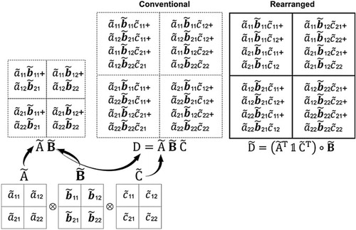
In order to solve this, we propose a modified matrix multiplication procedure, which preserves the initial structure of $\mathrm{\Delta }\mathbf{\text{A}}=\widetilde{\mathbf{\text{B}}}$ (result matrix in the top right of Figure 1).

The modified procedure delivers a result matrix $\widetilde{\mathbf{\text{D}}}$ that fully maintains the structure of $\widetilde{\mathbf{\text{B}}}$. ${\tilde{b}}_{11}$ is located in the first row and the first column, ${\tilde{b}}_{12}$ in the first row and the second column and so forth. Note that the sum of the modified, i.e. rearranged matrix multiplication and the sum of the conventional matrix multiplication are equal $\left(\sum \mathbf{\text{D}}=\sum \widetilde{\mathbf{\text{D}}}\right)$. The modified approach thus only reallocates values according to a specific structure. The modified result matrix that resembles the structure of $\widetilde{\mathbf{\text{B}}}$ can be calculated by applying the following equation: (10) $\widetilde{\mathbf{\text{D}}}=\left(\widetilde{\mathbf{\text{A}}}{}^{\mathrm{\prime }}\ast \text{𝟙}\ast {\widetilde{\mathbf{\text{C}}}}^{\mathrm{\prime }}\right)\circ \widetilde{\mathbf{\text{B}}}.$(10) In Equation 10, $\text{𝟙}$ stands for a matrix of the same dimension as $\widetilde{\mathbf{\text{A}}},\widetilde{\mathbf{\text{B}}}$ and $\widetilde{\mathbf{\text{C}}}$ containing only 1s. $\widetilde{\mathbf{\text{A}}}\mathbf{\ast }\text{𝟙}$ thus is a matrix with each cell giving the row sum of $\widetilde{\mathbf{\text{A}}}$. $\widetilde{\mathbf{\text{A}}}{}^{\mathbf{\prime }}$ indicates a transposition of $\widetilde{\mathbf{\text{A}}}$. It is important to note that the multiplication with $\widetilde{\mathbf{\text{B}}}$ is element-wise, which is termed the Hadamard product. Applying this type of matrix multiplication to the basic SDA identity as described in Equation 9a, we obtain the following: (10a) ${\mathbf{\text{A}}}_{4.\mathrm{eff}.2}=\left(\left(\widehat{\mathbf{\text{f}}}{\widehat{\mathbf{\text{x}}}}^{-1}\mathbf{\text{A}}\right){}^{\mathrm{\prime }}\text{𝟙}\left(\mathbf{\text{A}}\widehat{\mathbf{\text{y}}}\right){}^{\mathrm{\prime }}\right)\circ \mathrm{\Delta }\mathbf{\text{A}}$(10a) because (10b) $\widetilde{\mathbf{\text{A}}}=\widehat{\mathbf{\text{f}}}{\widehat{\mathbf{\text{x}}}}^{-1}\mathbf{\text{A}},$(10b) (10c) $\widetilde{\mathbf{\text{B}}}=\mathrm{\Delta }\mathbf{\text{A}},$(10c) (10d) $\widetilde{\mathbf{\text{C}}}=\mathbf{\text{A}}\widehat{\mathbf{\text{y}}},$(10d)

which results in (10e) $\sum \widehat{\mathbf{\text{f}}}{\widehat{\mathbf{\text{x}}}}^{-1}\mathbf{\text{A}}\mathrm{\Delta }\mathbf{\text{A}}\mathbf{\text{A}}\widehat{\mathbf{\text{y}}}=\sum \left(\left(\widehat{\mathbf{\text{f}}}{\widehat{\mathbf{\text{x}}}}^{-1}\mathbf{\text{A}}\right){}^{\mathrm{\prime }}\text{𝟙}(\mathbf{\text{A}}\widehat{\mathbf{\text{y}}}{)}^{\mathrm{\prime }}\right)\circ \mathrm{\Delta }\mathbf{\text{A}}.$(10e)

2.2.3. Aggregating the effects into a single SPLD result matrix

After structural decomposing the layer differences to layer $r=8$, we can aggregate the SPLD result matrices into the following summary matrices: (11a) ${\widehat{\mathbf{\text{x}}}}_{\mathrm{total}.\mathrm{eff}}=\sum _{k=0}^r{\widehat{\mathbf{\text{x}}}}_{k.\mathrm{eff}},$(11a) (11b) ${\mathbf{\text{A}}}_{\mathrm{total}.\mathrm{eff}}=\sum _{k=1}^r\sum _{m=1}^k{\mathbf{\text{A}}}_{k.\mathrm{eff}.m},$(11b) (11c) ${\widehat{\mathbf{\text{y}}}}_{\mathrm{total}.\mathrm{eff}}=\sum _{k=0}^r{\widehat{\mathbf{\text{y}}}}_{k.\mathrm{eff}},$(11c) (11d) $\sum _{k=0}^r\mathbf{\text{L}}{\mathbf{\text{D}}}_k={\widehat{\mathbf{\text{x}}}}_{\mathrm{total}.\mathrm{eff}}+{\mathbf{\text{A}}}_{\mathrm{total}.\mathrm{eff}}+{\widehat{\mathbf{\text{y}}}}_{\mathrm{total}.\mathrm{eff}},$(11d) where $k$ and $m$ are the running indices of layers and effects, respectively. Since this inter-model comparison is based on a common classification of 41 regions and 17 sectors, each of the three SPLD result matrices and the three summary matrices in Equations 11a–11c consist of 697 rows and 697 columns. The standard SPLD approach presented here differentiates effects stemming from $\mathbf{\text{x}}$, $\mathbf{\text{A}}$ and $\mathbf{\text{y}}$.

2.3. How to read SPLD result matrices

This section demonstrates the information provided by the SPLD approach by contrasting it with the information provided by the SDA approach. The example results illustrate the Eora-EXIOBASE decomposition of the public administration footprint of the EU-28. Figure 2 shows the calculated $\mathbf{\text{L}}$-effect (using SDA) and $\mathbf{\text{A}}$-effect (using SPLD) matrices. Please note that the SPLD result matrix, calculated as described in the previous sections, shows the aggregated $\mathbf{\text{A}}$-effects up to layer eight ($r=8$). The original result matrices (697 by 697) are aggregated into a sector-by-sector perspective (17 by 17). In order to further explain the interpretation of the SPLD results, we also select one hypothetical example path at the end of this subsection. But before reflecting on a single path, we examine the two different types of information that are incorporated in the result matrices.

FIGURE 2. L-effect matrix (above) versus A-effect matrix (below) from a sector perspective. Showing the structural decomposition results of the carbon footprint of the sector public administration of the EU-28, Eora-EXIOBASE pair, 2011.

Both matrices produce very different messages regarding the sectors that contribute to the overall deviation of the carbon footprint of the public administration sector. The SDA decomposition (Figure 2 top) of public administration’s carbon footprint shows that the major cause of difference stems from electricity emissions, i.e. paths that originate from electricity production. However, the aggregated effects (as observed in the $\mathbf{\text{L}}$-effect matrix) of all paths from sector 11 (electricity) to sector 17 (public administration) may actually be caused by differences in the downstream use structure of electricity, for example, the amount of electricity used by sector 6 (petroleum and chemicals) that is subsequently consumed by public administration. The effect shown with SDA for $l_{11,17}$ is unravelled with SPLD into single segments (meaning inter-industry deliveries $a_{i,j}$) of the related first-, second- or higher-order paths. In other words, the $\mathbf{\text{A}}$-effect perspective of SPLD reveals the actual inter-industry deliveries that are responsible for an effect, illustrating each sectors’ contribution to the paths that cause footprint differences, while the SDA approach using $\mathbf{\text{L}}$ highlights the sectors where the emissions originate from.

In contrast to SDA, the application of SPLD breaks down aggregated paths (e.g. electricity delivered via various intermediate consumers to public administration) into the constituting elementary inter-industry deliveries (elements in the $\mathbf{\text{A}}$ matrix). This allows us to identify the precise segments of the supply chains, i.e. inter-industry deliveries that are responsible for the differences. This information increase is only possible at the expense of losing the information on the origin of paths. While enabling us to quantify the effect that a single inter-industry delivery has on the aggregated carbon footprint, SPLD does not tell us which supply chain this inter-industry delivery (and hence the related effect) is associated to. Therefore, the results of the SDA and SPLD approaches should be seen as complementary, providing different types of information from different points of view.

Returning to the example result matrices in Figure 2, we see that the SDA approach points towards the electricity sector as a major source for variation in the EU-28 carbon footprint of public administration, while the SPLD approach identifies other sectors as being mainly responsible. The SPLD perspective, which uses the $\mathbf{\text{A}}$ matrix, illustrates that the noticeable effect of the electricity multiplier (see $l_{11,17}$ in Figure 2 top) is actually not rooted in the direct electricity input coefficients of the public administration sector (see element $a_{11,17}$ of the A-effect matrix in Figure 2). Instead, the main sources of the effects behind this multiplier seems to be the direct electricity input coefficients of the petroleum ($a_{11,6}$), metal products ($a_{11,7}$) and electricity sectors own use ($a_{11,11}$) as well as the manufacturing sectors supplying the public administration (like $a_{6,17}$ and $a_{7,17}$).

Next we focus on the example path shown in Figure 2 in order to deepen the understanding of the result matrices. We select a hypothetical second-order path that starts from the electricity sector (row 11) and ultimately delivers the final demand of public administration (column 17) via the intermediate consumption of electricity by the petroleum sector ($a_{11,6}$) and the intermediate consumption of petroleum by public administration ($a_{11,17}$). When applying the SDA approach, the effects of this path, which stem from the differences $\mathrm{\Delta }{a}_{11,6}$ and $\mathrm{\Delta }{a}_{6,17}$, are all attributed to element $l_{11,17}$ because the path and its related emissions originate from the electricity sector (row 11) and terminate in the public administration sector (column 17). When applying the SPLD method, the effects associated with the differences $\mathrm{\Delta }{a}_{11,6}$ and $\mathrm{\Delta }{a}_{6,17}$ are separated and allocated to the corresponding position in the technology matrix ($a_{11,6}$ and $a_{6,17}$). We should view the SPLD approach as a decomposition of the effects of the Leontief multipliers into the underlying technical coefficients.

2.4. About dependencies in SDA

One issue to be aware of is the dependency problem in SDA, where it is assumed that all variables are independent of each other (e.g. it is possible to modify $\mathbf{\text{A}}$ without modifying $\mathbf{\text{x}}$). Dietzenbacher and Los (2000) discuss this issue and provide examples for the case of the Netherlands. In our work, we could expect that there is some dependency between the size of $\mathbf{\text{f}}$ and the size of $\mathbf{\text{x}}$, as well as between $\mathbf{\text{f}}$ and $\mathbf{\text{A}}$, $\mathbf{\text{A}}$ and $\mathbf{\text{x}}$, and $\mathbf{\text{y}}$ and $\mathbf{\text{x}}$. However, there is no clear way to avoid the issue (Minx et al., 2011), hence care should be taken in interpretation of results. Nonetheless, we still feel that the application of SDA gives valuable insights, as has been shown widely through the literature (compare with Hoekstra and van den Bergh, 2002; Lenzen, 2016).

3. Results

The presentation of results starts with a description of the PLD results from each of the MRIO models and the calculated differences between each model pair, disaggregated by layers (Section 3.1). In a second step, we compare the decomposition results when applying structural decomposition analysis (SDA) using the $\mathbf{\text{L}}$ matrix with an SPLD analysis based on the $\mathbf{\text{A}}$ matrix (Section 3.2). In Section 3.3, we further decompose the results in order to investigate the origin of the observed differences in the $\mathbf{\text{A}}$ matrix across models. For example, we are able to determine whether the domestic or trade blocks in the $\mathbf{\text{A}}$ matrices contribute more to the overall difference; which countries’ $\mathbf{\text{A}}$ matrices show the largest effects; and which of the 17 sectors in the common classification system cause the most diverging carbon footprint values. Note that in the tables and figures of the results section, the MRIO database EXIOBASE is abbreviated as EXIO.

3.1. PLD results

Table 1 illustrates the results from the PLD undertaken with each of the four investigated MRIO models in the common classification. It shows the number of paths covered in each layer, up to layer eight. This is the number of paths that are implicitly structurally decomposed when applying SPLD analysis. The table also illustrates the absolute greenhouse gas emissions originating from each production layer. Note that the numbers for the EU-28 carbon footprints only refer to emissions embodied in products and exclude direct emissions of final demand, such as households.

TABLE 1. PLD of the EU-28 carbon footprint across the four MRIO models, in kt CO₂ equivalents, 2011.

Number of paths		Layer	Eora	EXIO	WIOD	GTAP
697^1 =	697	0	1,044,593	1,252,210	1,258,568	1,193,955
697^2 =	4.858E + 05	1	1,091,167	1,156,518	1,074,668	1,104,295
697^3 =	3.386E + 08	2	810,742	786,339	727,968	803,011
697^4 =	2.360E + 11	3	538,887	496,953	464,116	528,976
697^5 =	1.645E + 14	4	340,578	300,980	284,548	329,933
697^6 =	1.147E + 17	5	210,735	177,793	170,930	200,372
697^7 =	7.992E + 19	6	129,375	103,480	101,555	119,968
697^8 =	5.570E + 22	7	79,346	59,702	60,019	71,274
697^9 =	3.882E + 25	8	48,799	34,269	35,409	42,178
Aggregated total	3.888E + 25	∑(0 … 8)	4,294,223	4,368,245	4,177,781	4,393,962
Missing in SPLD	∞	9+	81,129	45,772	51,383	61,038
Total footprint	∑(∞)	∑(∞)	4,375,352	4,414,017	4,229,164	4,455,000

Table 1 shows that for each MRIO model around 3.9 × 10²⁵ paths and corresponding flows of greenhouse gas emissions are included in the analysis when considering all paths up to layer eight. For example, in the case of Eora, paths at layers zero to eight are responsible for around 4.3 billion tonnes of carbon emissions related to EU-28 final demand, whereas 81 million tonnes of emissions occur in layers nine and beyond. This means that in the case of Eora, the SPLD analysis covers more than 98% of the total EU-28 carbon footprint. For the other three MRIO models, the respective share is between 98% and 99%. Table 2 shows the layer differences ($\mathbf{\text{LD}}$) for each MRIO model pair by layer. The aggregated sum of the layer differences for each pair forms the basis of the SPLD analysis further below.

TABLE 2. Layer differences of EU-28 carbon footprints across the six model pairs, in kt CO₂ equivalents, 2011.

	Layer differences ($\mathbf{L}\mathbf{D}$)
Layer	Eora vs. EXIO	Eora vs. WIOD	Eora vs. GTAP	EXIO vs. WIOD	EXIO vs. GTAP	GTAP vs. WIOD
0	207,616	213,975	149,362	6,358	−58,255	64,613
1	65,352	−16,499	13,128	−81,851	−52,224	−29,627
2	−24,403	−82,774	−7,732	−58,370	16,672	−75,042
3	−41,934	−74,771	−9,911	−32,837	32,023	−64,860
4	−39,598	−56,030	−10,646	−16,432	28,953	−45,385
5	−32,942	−39,806	−10,363	−6,864	22,579	−29,443
6	−25,895	−27,820	−9,407	−1,925	16,488	−18,413
7	−19,644	−19,327	−8,072	318	11,572	−11,255
8	−14,529	−13,389	−6,620	1,140	7,909	−6,769
Aggregated Layer 0–8 net-difference:	74,022	−116,441	99,740	−190,463	25,717	−216,181
Layer 9+ difference:	−35,357	−29,746	−20,091	5,611	15,266	−9,655
Total footprint difference	38,665	−146,188	79,648	−184,853	40,983	−225,836

For example, the Eora-WIOD pair has an aggregated difference in layer zero to eight of approximately 116 million tonnes of CO₂ eq.. The total EU-28 carbon footprint difference between these models is 146 million tonnes of CO₂ eq., implying that around 80% of the footprint differences are covered, while 20% of the differences are located in layers higher than eight.

In this regard, it is important to highlight the possibility of having an aggregated difference larger than the total footprint difference. For example, the aggregation of differences across layers zero to eight of the Eora-EXIOBASE pair, with approx. 74 million tonnes CO₂ eq., is almost twice as large as the total EU-28 carbon footprint difference between the two models. This is due to the fact that positive and negative differences in different layers can compensate and cancel each other out.

Figure 3 provides a graphical illustration of the differences of each model pair by production layers. It is important to note that differences in Figure 3 are illustrated with their absolute values, disregarding whether the difference in Table 2 is positive or negative. This means that we can focus on the differences between the values generated with two different MRIO models, and positive or negative numbers can be turned around by simply switching the order within each model pair.

FIGURE 3. Absolute differences of the EU-28 carbon footprint by layers for six MRIO pairs, in kt CO₂ equivalents, 2011.

As Figure 3 shows, differences in layer zero are mainly related to model pairs involving Eora. The differences in higher layers seem to be more important for model pairs involving WIOD, where larger deviations are found for layer two and above. EXIOBASE is relatively similar to both GTAP and Eora in layers two and above. The Eora-GTAP pair is most homogenous and only shows larger deviations in layer zero.

3.2. $\mathbf{\text{L}}$ versus $\mathbf{\text{A}}$ perspectives

Section 3.1 illustrated the absolute differences in the EU-28 carbon footprint stemming from different production layers of each model pair. We now consider which part of the MRIO system actually causes the observed differences. Macro-scale comparisons of carbon footprint results have so far been undertaken applying the SDA approach using the $\mathbf{\text{L}}$ matrix (see Owen et al., 2014b for an analysis of Eora, GTAP and WIOD for the year 2007). Results for this approach, based on 2011 data, are illustrated in the upper part of Figure 4. We compare the outcome of the SDA with the result from applying SPLD, which uses the $\mathbf{\text{A}}$ matrix (lower part of Figure 4).

FIGURE 4. Results from SDA (above) versus SPLD (below) across the six model pairs, in kt CO₂ equivalents, 2011.

Figure 4 illustrates that the aggregated results from the SPLD versus SDA analysis are very similar. The main difference is that total absolute effects of both approaches are not identical because SPLD structurally decomposes the differences up to layer eight, whereas SDA considers all production layers. For example, for the case of the Eora-WIOD pair, the difference between the total effect was calculated by the SDA approach is approximately 30 million tonnes CO₂ eq. larger than the total effect calculated applying the SPLD approach. However, we expect that using the SPLD as the starting point for further analysis (see Sections 3.3 and 3.4) delivers comparable results to the SDA, even though not all paths are included.

As Figure 4 shows, in many cases, the effects stemming from the $\mathbf{\text{L}}$ matrix (above) or $\mathbf{\text{A}}$ matrix (below), the $\mathbf{\text{y}}$-effect (resp. $\mathbf{\text{A}}$/$\mathbf{\text{L}}$-effect) and the $\mathbf{\text{x}}$-effect compensate for each other, leading to relatively smaller total effects. Taking again the Eora-WIOD pair as an example, both SDA and SPLD suggest that if differences in the $\mathbf{\text{A}}$ (or $\mathbf{\text{L}}$) matrix as well as the $\mathbf{\text{x}}$-effect are negative, differences in $\mathbf{\text{y}}$ will be positive, thus leading to a relatively smaller total difference.

To further investigate in which parts of the $\mathbf{\text{L}}$ and $\mathbf{\text{A}}$ matrices, the observed effect is being generated, we start with a country level analysis. As mentioned above, the results of SPLD are matrices in the format of 697 rows and 697 columns. We aggregate to a country-by-country format to provide an overview of those countries causing the major deviations. Furthermore, we illustrate which blocks of the matrices, i.e. domestic blocks versus trade blocks, have the largest effect on the differences in EU-28 carbon footprints. The sum of these matrices across all layers is identical to the value of the overall $\mathbf{\text{A}}$-effect as illustrated in Figure 4.

In order to illustrate the difference in perspective when using the $\mathbf{\text{A}}$ matrix instead of the $\mathbf{\text{L}}$ matrix, we compare the country aggregated A-effect matrix with the $\mathbf{\text{L}}$-effect matrix for the example pair of Eora and EXIOBASE (Figure 5). Note that the sums of the areas (bubbles) in Figure 5 are scaled to the same totals for ease of comparison.

FIGURE 5. L-effect matrix (above) versus A-effect matrix (below) from a country perspective including the domestic (DOM), import (IM) and export (EX) blocks on the right, Eora-EXIO pair, 2011.

Analysing the deviations between the Eora and EXIOBASE models from the perspective of the $\mathbf{\text{L}}$ matrix shows that the domestic blocks in the multi-regional table cause the largest deviations, notably for Germany, the UK, Poland and Italy within Europe, and China in the non-European countries. Large effects can also be observed for some import and export blocks, most notably exports from China, the Rest of the World (RoW) region and from Russia. The $\mathbf{\text{L}}$ perspective would therefore suggest prioritising the harnisation of data in some of the trade blocks in order to align the resulting carbon footprint for the EU-28.

However, the perspective of the $\mathbf{\text{A}}$ matrix in Figure 5 illustrates that the noticeable trade effects stem from deviations in the domestic tables of these countries and regions. From the $\mathbf{\text{A}}$ perspective, differences between the Eora and EXIOBASE models are foremost found in the domestic block of China. The aggregated $\mathbf{\text{L}}$-effect of China’s domestic block accounts for approximately 87 million t CO₂ eq. compared to around 415 million t CO₂ eq. for the aggregated $\mathbf{\text{A}}$-effect. Also in the $\mathbf{\text{A}}$ perspective, exports from China to the other regions show deviations, and these are significantly smaller compared to the $\mathbf{\text{L}}$ perspective. The same pattern can be observed for the cases of the RoW region and Russia. This suggests that the differences in the trade blocks observed in the $\mathbf{\text{L}}$ perspective could be reduced by harmonising data in the domestic blocks of the respective countries. Within the EU, the same problematic domestic blocks are identified in the $\mathbf{\text{A}}$ perspective and the $\mathbf{\text{L}}$ perspective, i.e. Germany, the UK, Poland and Italy.

3.3. SPLD results: country and sector hot-spots across MRIO models

In the following section, we concentrate our analysis on the effects stemming from the $\mathbf{\text{A}}$ matrix in order to further investigate which parts of the domestic and foreign blocks cause the largest deviations in the EU-28 carbon footprint results.

Figure 6 provides a first overview across the six model pairs, illustrating the effect of the domestic block (DOM) versus the effects stemming from the import blocks (IM) and export blocks (EX) of each country in the common classification.

FIGURE 6. Effects from the domestic (DOM), import (IM) and export (EX) blocks of the A matrix, six model pairs and mean across all models, 2011.

Figure 6 confirms the general trend observed in Figure 5, i.e. that the domestic block contributes higher absolute differences in the EU-28 carbon footprint compared to the trade block. This holds true for all six model pairs. For non-EU countries, export blocks are more important than import blocks, whereas it is the other way around for EU countries where there are larger deviations in their import blocks. This result is unsurprising given that EU countries are generally net-importers of embodied GHG emissions (Peters et al., 2011b; Tukker et al., 2016). China stands out as the country with the strongest deviations. More disaggregated heat maps, showing the full trade relations between countries for each model pair, can be found in the Supplementary Information SI 1.

In order to further pin down, the sources of observed differences, we can zoom into each of the domestic blocks. As an example, we take a closer look at China’s domestic block to identify the main sectors responsible for these differences (Figure 7). In the case of the Eora-EXIOBASE pair, the total $\mathbf{\text{A}}$-effect of China’s domestic block accounts for around 415 million t CO₂ eq.. This effect is mainly related to differences in the electricity input coefficients (row i.e. code 11) of the petroleum, metal product and electrical machinery sector (columns i.e. codes 6, 7 and 8). As Figure 7 shows, in terms of the effects stemming from China’s domestic block, intermediate inputs of electricity seem to be a major source of variation across all MRIO pairs. Other key sectors of the Chinese economy which show significant variations in the input structures are metal products and petroleum and chemical products.

FIGURE 7. $\mathbf{\text{A}}$-effect of the domestic block of China in a sector perspective for all six model pairs, 2011.

After investigating a single domestic block in more detail, in Figure 8, we show a sector perspective on the total $\mathbf{\text{A}}$-effect. Figure 8 therefore contains a sector aggregation corresponding to the geographical $\mathbf{\text{A}}$-effect matrices as shown in the lower part of Figure 5.

FIGURE 8. $\mathbf{\text{A}}$-effect matrix in an aggregated sector perspective for all countries and all six model pairs, 2011.

Figure 8 illustrates that in the overall sector perspective, the effects stemming from the electricity input coefficients are less pronounced. In particular, the variations in the petroleum (row, i.e. code 6) and mining sector coefficients have strong effects on the variations between the EU-28 carbon footprints. With regard to the effects stemming from differences in the petroleum sectors’ own use coefficients $a_{6,6}$ (row and column six), we find that Germany (an average difference across all model pairs of around 21 million t CO₂ eq.) and the rest of the world region (19 million t CO₂ eq.) in particular contribute the largest effects (see supplementary information SI 2 for the full results table). The effects stemming from differences in the input coefficients of mining to petroleum ($a_{2,6}$) are foremost driven by differences in the domestic input coefficients of Russia (an average difference across all model pairs of around 22 million t CO₂ eq.) and the rest of the world region (25 million t CO₂ eq.) (see supplemental information SI 2 for the full results table).

4. Discussion

The analysis undertaken in this paper showed that the domestic blocks have a stronger effect on the variations of carbon footprints of the EU-28 than the trade blocks. This observation holds true for all six model pairs. On average we find the domestic blocks are responsible for around 56% of the absolute carbon footprint variations that stem from differences in the technology matrix. Our results therefore contrast earlier findings based on SDA. SPLD therefore provides a complementary response to the question: ‘which parts of the MRIO system cause the highest deviations in footprint results?’. We have illustrated that the noticeable trade effects observed through analysis of the $\mathbf{\text{L}}$ matrix actually stem from the deviations in the domestic tables of these countries and regions.

With regard to the question of which sections of the technology matrices yield the highest return on investment in terms of carbon footprint harmonisation efforts, we identified key hot spots. The top six domestic blocks that have the greatest impact on the EU-28 carbon footprint are those of China, Germany, RoW, UK, Italy and Russia. China’s domestic block effects are foremost a result of the differences in the electricity input coefficients. The effects of the domestic block of Germany are essentially due to differences in the input coefficients of mining products to the petroleum sector.

The next figure provides an overview of the geographical blocks in the technology matrix that have the largest ‘return on investment’ with regard to model harmonisation. It shows the Top-11 regional blocks (domestic and import blocks) that contribute most to the total average $\mathbf{\text{A}}$-effect across all MRIO model pairs. Hatched bars represent domestic blocks and dotted bars are import blocks. The grey bars depict the cumulative or combined effect. For example, the grey bar behind the hatched domestic RoW block stands for the sum of the domestic block of China (7%), the domestic (6%) and import (7%) block of Germany and the domestic block of RoW (6%), which accounts for approximately 26% of the average absolute $\mathbf{\text{A}}$-effect.

As Figure 9 shows the Top-11 blocks cumulate to almost 50% of the total average $\mathbf{\text{A}}$-effect across all MRIO model pairs. On average, the top six domestic blocks account for almost 30% of the absolute effects that stem from differences in the technology matrices. With regard to the import blocks, the largest effects on the differences in EU-28 carbon footprints are those of imports to Germany, Italy, UK, France and the Netherlands. Germany’s import block effects are mainly driven by differences in the input (i.e. import) coefficients of China (import of petroleum and metal products to public administration in Germany) and RoW (import of mining products to the petroleum sector in Germany) (see supplementary information SI 2 for the full results table). In summary, our analysis finds that the harmonisation of the top five import blocks plus the top six domestic blocks would decrease the absolute effects of the technology matrices by more than 50%. This would help to decrease the variations of the EU-28 Carbon Footprints across the various MRIO models significantly.

FIGURE 9. Most important blocks in terms of average absolute A-effect across all MRIO model pairs.

5. Conclusions

In this paper, we introduced a new method, SPLD, for identifying sources of differences of macro-level footprints. The SPLD method aims at complementing the existing approaches of SDA and SPDA.

We have demonstrated that SPLD is a very useful technique in determining the difference between MRIO databases. Its ability to trace the causes of differences to individual cells within the technology matrix is a clear advantage over traditional SDA, which treats the Leontief inverse as a single layer connecting origin of production and point of final consumption. We believe that SPLD has many potential applications beyond this paper. For example, when used for year-on-year decomposition assessments, SPLD will be able to determine the contribution that an annual change to the production recipe of a specific product has had on the change in the overall footprint.

5.1. Relevance for MRIO construction and evidence-based policy

The results presented in this paper provide a wealth of information for MRIO developers. The results highlight that the domestic flows have a larger contribution to the difference in MRIO databases than the trade flows. Clearly there is a need for consistency of source data, particularly, in the domestic use tables from the major economies (for example, China or Germany). We thus join Wiedmann et al. (2011) in calling for improvements in the gathering and assessment of economic data. We also suggest that prioritising domestic data is more important than prioritising information on trade flows. Within the domestic flows, traditional key emitting sectors stand out, and given the well-studied and singular nature of the electricity sector, it is of some concern that this sector is still causing significant variation across the MRIO models.

If consumption-based carbon accounts are to be used as evidence in the design of targeted policy responses it is essential that the results from MRIO analyses are trustworthy. Policy makers must understand the level of robustness in the information they are using to derive policies. Our results suggest that even when there is similarity between country level consumption-based accounts produced by different databases, there is difference in distribution of impact at various stages of the supply chain. This would have implications on policy measures that are designed to cause changes at important points along a product supply chain. For example, evidence from one MRIO database might suggest that a material efficiency policy measure, which focuses on reducing the rolled steel in cars, would have negligible effect, whereas a different database might imply that this stage in the supply chain produces a large portion of product’s overall emissions impact and that the policy measure would have a useful effect. We suggest that evidence based on calculations of the impact embodied in trade, or the impact of the final good are more robust than calculations made at single production layers. This implies that evidence from MRIOs could be used for trade policy and for demand-side strategies such as reducing food waste, dietary changes and changes in individual mobility, such as the promotion of public transport and car-sharing.

5.2. Limitations and directions for further research

As described above, SPLD has several advantages compared to the existing SDA and SPDA approaches. However, limitations need to be addressed. First, the SPLD algorithm in its current form is relatively time-consuming. For each pairwise-comparison, more than 10,000 matrix multiplications (applying the rearranged multiplication approach) need to be performed when structurally decomposing the footprint differences up to layer eight. Hence limited computation time or power can pose a challenge to the application of SPLD. The SDA approach is therefore preferable for providing overviews of the main differences between MRIO databases. Second, SPLD works on the level of production layers and is therefore unable to elucidate differences between MRIO databases of single structural paths. If the objective of the study is to analyse supply chains of single product groups and compare them across different MRIO models, SPDA would be the preferred method.

This paper focused on introducing the SPLD method to investigate the impact of differences in the basic data underlying the various existing MRIO systems on the overall result of footprint indicators, taking the carbon footprint of the EU-28 as an example. Our analysis delivered new insights into determining which deviations between different MRIO databases cause substantial differences in footprint results. The next crucial step will be to investigate why these deviations are being observed. This will require comparing the original data sources applied to construct the national input–output tables of countries causing major differences, such as the Chinese domestic table. Furthermore, this will require a systematic comparison of the assumptions and data manipulation procedures applied to establish the consistent MRIO system, for example, finding out whether the national or the trade data are being given priority in the data adjustment techniques. Finally, further investigations will be required on the impacts of different levels of aggregation in the original MRIO systems and how these translate into differences in results in more aggregated common classifications.

Supplemental data

Supplemental material for this article includes: (SI 1) $\mathbf{\text{A}}$-effect heat maps in a country perspective for all six model pairs; (SI 2) a CSV file containing a list of the detailed (697 by 697) average (across all model pairs) $\mathbf{\text{A}}$-effect values which can be converted into a PIVOT table; (SI 3) an XLSX file containing the data that has been used for the bubble heat maps.

Acknowledgements

We would like to thank three anonymous reviewers for their insightful comments on the paper.

Disclosure statement

No potential conflict of interest was reported by the authors.

Additional information

Funding

This research was financed by the European Commission under the FP7 project “Carbon-Cap” (Grant number 603386). Anne Owen's time was supported by the research programme of the UK Energy Research Centre, supported by the UK Research Councils under [EPSRC award EP/L024756/1] and the RCUK Energy Program's funding for the Centre for Industrial Energy, Materials and Products [grant reference EP/N022645/1].

References

- Ang, B.W. (2004) Decomposition Analysis for Policymaking in Energy: Which is the Preferred Method? Energy Policy, 32, 1131–1139. doi: 10.1016/S0301-4215(03)00076-4
- Arto, I., J.M. Rueda-Cantuche, and G.P. Peters (2014) Comparing the GTAP-MRIO and WIOD Databases for Carbon Footprint Analysis. Economic Systems Research, 26, 327–353. doi: 10.1080/09535314.2014.939949
- Dietzenbacher, E. and B. Los (1998) Structural Decomposition Techniques: Sense and Sensitivity. Economic Systems Research, 10, 307–324. doi: 10.1080/09535319800000023
- Dietzenbacher, E. and B. Los (2000) Structural Decomposition Analyses with Dependent Determinants. Economic Systems Research, 12, 497–514. doi: 10.1080/09535310020003793
- Dietzenbacher, E., B. Los, R. Stehrer, M. Timmer, and G. de Vries (2013). The Construction of World Input–Output Tables in the WIOD Project. Economic Systems Research, 25, 71–98. doi: 10.1080/09535314.2012.761180
- Giljum, S., H. Wieland, S. Lutter, M. Bruckner, R. Wood, A. Tukker, and K. Stadler (2016) Identifying Priority Areas for European Resource Policies: A MRIO-Based Material Footprint Assessment. Journal of Economic Structures, 5, 1–24. doi: 10.1186/s40008-016-0048-5
- Hoekstra, R. and J. van den Bergh (2002) Structural Decomposition Analysis of Physical Flows in the Economy. Environmental and Resource Economics, 23, 357–378. doi: 10.1023/A:1021234216845
- Inomata, S. and A. Owen (2014). Comparative Evaluation of MRIO Databases. Economic Systems Research, 26, 239–244. doi: 10.1080/09535314.2014.940856
- Kagawa, S. and H. Inamura (2001) A Structural Decomposition of Energy Consumption Based on a Hybrid Rectangular Input–Output Framework: Japan's Case. Economic Systems Research, 13, 339–363. doi: 10.1080/09535310120089752
- Lenzen, M. (2016) Structural Analyses of Energy Use and Carbon Emissions – An Overview. Economic Systems Research, 28, 119–132. doi: 10.1080/09535314.2016.1170991
- Lenzen, M. and R.H. Crawford (2009) The Path Exchange Method for Hybrid LCA. Environmental Science & Technology, 43, 8251–8256. doi: 10.1021/es902090z
- Lenzen, M., D. Moran, K. Kanemoto, and A. Geschke (2013) Building EORA: A Global Multi-Region Input–Output Database at High Country and Sector Resolution. Economic Systems Research, 25, 20–49. doi: 10.1080/09535314.2013.769938
- Llop, M. and X. Ponce-Alifonso (2015) Identifying the Role of Final Consumption in Structural Path Analysis: An Application to Water Uses. Ecological Economics, 109, 203–210. doi: 10.1016/j.ecolecon.2014.11.011
- Minx, J.C., G. Baiocchi, G.P. Peters, C.L. Weber, D. Guan, and K. Hubacek (2011) A “Carbonizing Dragon”: China’s Fast Growing CO2 Emissions Revisited. Environmental Science & Technology, 45, 9144–9153. doi: 10.1021/es201497m
- Moran, D. and R. Wood (2014) Convergence Between the Eora, WIOD, EXIOBASE, and OpenEU's Consumption-Based Carbon Accounts. Economic Systems Research, 26, 245–261. doi: 10.1080/09535314.2014.935298
- OECD (2015). OECD Inter-Country Input–Output (ICIO) Tables, Edition 2015. Paris, Organisation for Economic Co-operation and Development.
- Owen, A., K. Steen-Olsen, J. Barrett, and A. Evans (2014a) Matrix Difference Statistics and Their Use in Comparing Input–Output Databases (Paper presented at the International Input–Output Conference 2014, Lisbon, Portugal).
- Owen, A., K. Steen-Olsen, J. Barrett, T. Wiedmann, and M. Lenzen (2014b). A Structural Decomposition Approach to Comparing MRIO Databases. Economic Systems Research, 26, 262–283. doi: 10.1080/09535314.2014.935299
- Owen, A., R. Wood, J. Barrett, and A. Evans (2016) Explaining Value Chain Differences in MRIO Databases Through Structural Path Decomposition. Economic Systems Research, 28, 243–272. doi: 10.1080/09535314.2015.1135309
- Peters, G.P. and E.G. Hertwich (2008) CO2 Embodied in International Trade with Implications for Global Climate Policy. Environmental Science & Technology, 42, 1401–1407. doi: 10.1021/es072023k
- Peters, G.P., R. Andrew, and J. Lennox (2011a) Constructing an Environmentally-Extended Multi-Regional Input–Output Table Using the GTAP Database. Economic Systems Research, 23, 131–152. doi: 10.1080/09535314.2011.563234
- Peters, G.P., J.C. Minx, C.L. Weber, and O. Edenhofer (2011b) Growth in Emission Transfers Via International Trade from 1990 to 2008. Proceedings of the National Academy of Sciences, 108, 8903–8908.
- Steen-Olsen, K., A. Owen, J. Barrett, D. Guan, E.G. Hertwich, M. Lenzen, and T. Wiedmann (2016) Accounting for Value Added Embodied in Trade and Consumption: An Intercomparison of Global Multiregional Input–Output Databases. Economic Systems Research, 28, 78–94. doi: 10.1080/09535314.2016.1141751
- Steen-Olsen, K., A. Owen, E.G. Hertwich, and M. Lenzen (2014) Effects of Sector Aggregation on CO2 Multipliers in Multiregional Input–Output Analyses. Economic Systems Research, 26, 284–302. doi: 10.1080/09535314.2014.934325
- Sun, J. (1998) Changes in Energy Consumption and Energy Intensity: A Complete Decomposition Model. Energy Economics, 20, 85–100. doi: 10.1016/S0140-9883(97)00012-1
- Tukker, A., T. Bulavskaya, S. Giljum, A. de Koning, S. Lutter, M. Simas, K. Stadler, and R. Wood (2016) Environmental and Resource Footprints in a Global Context: Europe’s Structural Deficit in Resource Endowments. Global Environmental Change, 40, 171–181. doi: 10.1016/j.gloenvcha.2016.07.002
- Tukker, A., A. de Koning, R. Wood, T. Hawkins, S. Lutter, J. Acosta, J.M. Rueda Cantuche, M. Bouwmeester, J. Oosterhaven, T. Drosdowski, and J. Kuenen (2013) Exiopol–Development and Illustrative Analyses of a Detailed Global MR EE SUT/IOT. Economic Systems Research, 25, 50–70. doi: 10.1080/09535314.2012.761952
- Wiedmann, T. and J. Barrett (2013) Policy-Relevant Applications of Environmentally Extended Mrio Databases–Experiences from the UK. Economic Systems Research, 25, 143–156. doi: 10.1080/09535314.2012.761596
- Wiedmann, T.O., M. Lenzen, and J.R. Barrett (2009) Companies on the Scale. Journal of Industrial Ecology, 13, 361–383. doi: 10.1111/j.1530-9290.2009.00125.x
- Wiedmann, T., H.C. Wilting, M. Lenzen, S. Lutter, and V. Palm (2011) Quo Vadis Mrio? Methodological, Data and Institutional Requirements for Multi-Region Input–Output Analysis. Ecological Economics, 70, 1937–1945. doi: 10.1016/j.ecolecon.2011.06.014
- Wilting, H.C. (2012) Sensitivity and Uncertainty Analysis in Mrio Modelling; Some Empirical Results with Regard to the Dutch Carbon Footprint. Economic Systems Research, 24, 141–171. doi: 10.1080/09535314.2011.628302
- Wood, R. and M. Lenzen (2009) Structural Path Decomposition. Energy Economics, 31, 335–341. doi: 10.1016/j.eneco.2008.11.003
- Wood, R., 2009. Structural Decomposition Analysis of Australia's Greenhouse Gas Emissions. Energy Policy, 37, 4943–4948. doi: 10.1016/j.enpol.2009.06.060
- Wood, R., K. Stadler, T. Bulavskaya, S. Lutter, S. Giljum, A. de Koning, J. Kuenen, H. Schütz, J. Acosta-Fernández, A. Usubiaga, M. Simas, O. Ivanova, J. Weinzettel, J. Schmidt, S. Merciai, and A. Tukker (2015) Global Sustainability Accounting – Developing Exiobase for Multi-Regional Footprint Analysis. Sustainability, 7, 138–163. doi: 10.3390/su7010138