Tools for reconstructing the bilateral trade network: a critical assessment

ABSTRACT

This study critically assesses the performances of the Gravity Model (GM) and of the RAS algorithm for the bilateral flow intensity estimations and link prediction. The main novelty is the application of these methodologies to reconstruct the network topology with a minimum amount of information. Moreover, we implement a multi-layer analysis to provide a comprehensive and robust framework, by testing several food commodities, over the period 1986–2013. The main outcomes suggest that the RAS algorithm outperforms the Gravity Model in the estimations of the bilateral trade flows, importantly guaranteeing the balance constraints (i.e. global import equals global export), while GM generates lower relative errors, but it underestimates total global flows. Both RAS and GM can be applied to accurately recover the network architecture. The implications of our study encompass a wide range of applications: systemic-risk assessment, creation of new databases, and scenario analyses to support policy decisions.

KEYWORDS:

• International agricultural trade
• networks
• RAS algorithm
• gravity model
• trade forecasting and simulation

JEL:

• C13
• C18
• C67
• F14
• F17
• L14
• Q17

1. Introduction

Global trade has grown at twice the rate of the global economy since the 1990s, bearing benefits and risks (Niepmann and Schmidt-Eisenlohr, 2017; Moon, 2018). In particular, around 23% of the total food for human consumption is traded internationally and the amount of food calories traded in the international food trade network (IFTN) has more than doubled since 1986 (D'Odorico et al., 2014). During the past decades, the agro-trade structure changed significantly, in terms of major players involved, flow size, and number of links (Fagiolo et al., 2010). The expansion and change of the IFTN, the increasing dependence from markets for many countries, and the fast growth of population have attracted the attention of researchers and politicians. Indeed, understanding the structure and the evolution of the IFTN (Distefano et al., 2018b) has remarkable implications in several dimensions, such as: trade policy (Giordani et al., 2016), water resource management (Tamea et al., 2014; Tuninetti et al., 2017), shock propagation (Distefano et al., 2018a), land use (e.g. Dell'Angelo et al., 2017), energy (White et al., 2018), and climate change (Babiker, 2005).

Two tied issues are of foremost importance in this context, to say: (a) a reliable and robust estimation of bilateral trade flow intensities, and (b) the reconstruction of the IFTN topology with a minimum amount of information. Point (a) is crucial because an accurate estimation of trade volumes – in physical (e.g. tonnes) and monetary terms (e.g. US dollars) – allows one to properly compute other relevant indicators (e.g. water/energy/land footprint, market competitiveness, and so on). Point (b) is essential to understand network dynamics and to build credible scenarios. Indeed, in many cases, bilateral trade data are not available nor reliable, while information on national aggregates (i.e. total imports and exports) are based on official accounts and are easier to obtain. Therefore, the application of a reliable methodology that accurately recovers the trade architecture (i.e. the network topology) from national aggregates is crucial for several reasons, such as: identification of the key players and market structure, forecast scenarios and analyses, and systemic-risk assessment. We aim at contributing to both issues by applying two well-known methodologies – viz. the gravity model and the RAS algorithm.

Since its introduction in the 1960s (e.g. Ball, 1967) the gravity model (henceforth GM) has been extensively used in international trade research to estimate the amount of monetary bilateral exchanges for its empirical robustness and explanatory power (e.g. Kepaptsoglou et al., 2010; Fally, 2015), although its theoretical foundation is still debated (Krugman, 1980; Chaney, 2018). Several studies used GM to analyse country-pair trade flows for specific agricultural products (e.g. Sarker and Jayasinghe, 2007) and at different scales (e.g. Anderson et al., 2016). Analogously, the bi-partitive RAS algorithm (McDougall, 1999; Robinson et al., 2001; Ahmed and Preckel, 2007) has been extensively adopted to update the input–output tables (Lahr and De Mesnard, 2004; Wiebe and Lenzen, 2016), to forecast the evolution of intermediate trading structure (Dietzenbacher and Hoekstra, 2002; Tarancón and Rio, 2005), and for structural dynamic analyses (Dietzenbacher and Hoekstra, 2002; D'Alessandro et al., 2018).

It is worth noting that sometimes GMs and RAS algorithms are applied in series (Gallego and Lenzen, 2009), using the results of GM as initial condition before running the RAS algorithm (e.g. Sargento et al., 2012; Pinilla et al., 2018), but almost no studies have been carried out so far to critically evaluate their performances in terms of estimation accuracy and predictive power. We aim at filling this gap. Note that our aim is motivated by the fact that usually the GM is applied in isolation to calibrate the general equilibrium models (Ivus and Strong, 2007; Balistreri and Hillberry, 2008). On the other hand, the RAS procedure is mostly applied only in the input–output (IO) framework, while we show that it can be fruitfully extended also in the network contests. Indeed, although we do not use the common IO structure (since in our database there are no sectors), we represent the international trade network, at the country-scale, in a matrix form in order to apply the RAS procedure, as explained in the next Section. We also provide evidence that both GM and RAS are suitable to infer the network topology and to estimate the corresponding flows.

These reasons lead us to investigate the following research questions: (i) what is the best technique to estimate the intensity of bilateral trade flows, knowing the topology of the network? (ii) how to obtain a reliable reconstruction of the IFTN connectivity structure, with a limited amount of information, when the topology is unknown? (iii) does the procedure of item aggregation entail remarkable biases in the estimation accuracy? With respect to the point (i) this is the first cross-methodological comparison for the estimation of international trade flows. In the literature, few attempts applied both methodologies – GM and RAS – to improve the estimations of the links' weights (e.g. Bon, 1984; Ahmed and Preckel, 2007), but none provided a comprehensive, fair (i.e. using exactly the same input data), and detailed comparison framework, where the strengths and weaknesses of the two methods are critically examined.

To the best of our knowledge, the procedure applied to face point (ii) is a novelty – although previous studies attempted to estimate the inner part of a trade matrix under limited information (Lenzen et al., 2013) – because we try to reconstruct the topology of the trade network assuming no prior knowledge. The possibility to properly recover the network architecture has manifold implications and it is particularly relevant because trade structure is unknown for many commodities, other than food. We apply the aforementioned methods to infer the network architecture by using only aggregate values, such as country's imports and exports. To respond to point (iii), we implement robustness checks by extending the study to aggregated networks other than single-commodity layers. To do so, we repeat our procedure with different units of measure, such as monetary values (in US dollars) and virtual water (in ${\mathrm{m}}^3$).¹ Indeed, the choice of food commodities as case study is motivated by the possibility to apply alternative unit of measures, then improving the understanding of the potential bias due to item aggregation. However, although our analysis focused on an estimation problem within the IFTN, it is generalisable and can be applied to any other task where any type of commodity flows (in various units and scales) are to be estimated.

The current study is structured as follows: Section 2 presents the dataset and Section 3 describes the two methodologies and explains the procedure of topological reconstruction. Section 4 reports the main results, while Section 5 discusses the main implications and the importance of a multi-layer approach. Finally, Section 6 draws the main conclusions.

2. Data

Trade data are taken from the publicly-available Food and Agricultural Organization of the United Nations' online database (FAOSTAT),² which reports the trade flow among 254 countries for several commodities, from 1986 to 2013.³ We select five basic raw food products (wheat, maize, rice milled, barley, and soy-beans) because they cover more than 55% of the global calories intake (D'Odorico et al., 2014). The bilateral exchanges larger than 1000 tonnes are selected; this operation does not alter the structure of the network since small fluxes cover, overall, less than 0.3% of the global trade flow.

FAOSTAT provides physical (tonnes) values of the bilateral trade exchanges from which we build the matrix F whose entries are the amount of exchange between any single exporter j and importer k in tonnes ($F_{jk}$). We represent the IFTN as a matrix where entries are the bilateral trade flows, and row and column sums are the total export ($E_j=\sum _k{F}_{jk}$) and import ($M_k=\sum _j{F}_{jk}$) of each country, respectively. Note that we build a different bilateral trade matrix F for each food commodity (also indicated as a layer) to assess them separately. In a second phase, we analyse the aggregate trade matrix determined by the (cell-by-cell) sum of all the layers included in this study. The global agro-trade system can be seen as a multi-layer network, also known as a world trade web (e.g. Ledwoch et al., 2018), where countries are represented through nodes and commercial relations through weighted and directed links (i.e. represented by a cell entry). Each layer pertains to a different commodity and describes the strength of countries relations.

In order to perform the assessment for differently weighted trade networks, we built the monetary value network and the virtual water trade network. The vectors of the coefficient of conversions, of each physical flow (in ton) departing from node j to node k, are represented by the average country exporting price (US dollars per ton) and by the virtual water content (${\mathrm{m}}^3$/ton of each exporting country). Unit prices are available from the FAOSTAT database, while the virtual water content has been derived from the WaterSTAT database (https://waterfootprint.org/en/resources/waterstat/). Note that we operate a supply-side (or row-type) conversion from tonnes to the other unit of measures, meaning that the coefficients of conversion are characteristic of the exporters and then we extend the operation to the relative importing partners. For example, we compute the matrix of bilateral trade matrix in dollar as $\mathbf{V}=\mathrm{diag}(\pi )\cdot \mathbf{F}$, from the vector of average exporting price π,⁴ where ‘diag’ means diagonal matrix. This operation allows one to aggregate more layers (represented by each food commodity) through a common unit of measure and to compare the reliability of GM and RAS at different scales.⁵

For the sake of synthesis, we only show the results for the monetary networks (V), while the results for virtual water for each commodity layer (tonnes) are reported in the Supplementary Materials (SM.1), which is available online.

3. Methods

The study is composed by two different parts: first, we compare the performances of GM and RAS in terms of estimating accuracy given a known topology (i.e. the structure of bilateral trade); second, we evaluate the predictive power assuming that the topology is unknown, to say the possibility to reconstruct the (weighted) links that actually composes the real IFTN architecture (see Section 3.3). Note that, in the first part, to ensure a fair comparison of the estimation power of each tool, we use the same set of regressors (geographical distance and country's export and import) in both cases.

To evaluate the estimating accuracy we use the following steps: first, defining the topology of the IFTN on the base of real data, hence excluding the links that actually do not exist (zeros); second, estimating the bilateral trade flows via RAS and GM, separately; and, finally, computing the coefficient of determination ($R^2$) both in linear and logarithmic terms to have a measure of the estimative accuracy. Note that the computation of a linear and logarithmic $R^2$ aims at discriminating which method is better for catching the absolute values of the flow ($R_{lin}^2$) and which one, instead, provides the estimations that are closer, in relative terms (percentage), to the real ones ($R_{log}^2$). This is of particular interest when the system shows a substantial dispersion of flows distribution, to say when there are both very large and very small flows of trade exchange. This holds true in case of the IFTN and in most of the international markets, in general. The adjusted coefficient of determination ($R^2$) is defined as (1) $R^2=1-\frac{\sum _j\sum _k(y_{jk}-{\hat{y}}_{jk}{)}^2}{\sum _j\sum _k(y_{jk}-\overline{y}{)}^2}\cdot \frac{N-1}{N-n_x}$(1) where $R^2$ that takes into account the number of regressors ($n_x$) with respect to the number of observations (N, viz. the overall number of links), ${\hat{y}}_{jk}$ is the estimated flow, and $\overline{y}$ is the average observed flow. In the linear case we have that $y_{jk}=F_{jk}$, while in case of logarithm it becomes $y_{jk}=$ ln($F_{jk}$). Note that adjusting the $R^2$ by the number of observations and regressors is necessary to allow a fair comparison and then to correct the estimating accuracy in case one tool uses more information (i.e. more observations).

Another relevant point is related to the procedure of layer (i.e. item) aggregation. After the selection of a common unit of measure – to obtain the aggregate network with the 5 crops of this study together – we operate two different types of aggregation:

1. ‘ex-post sum-up’: single crop-level estimation in tonnes, then application of the coefficient of conversion (i.e. unit of measure) to the estimated values (with RAS and GM separately), and finally aggregation by summation of the five estimated layers (i.e. layers summation after estimation of the single-commodity network);

2. ‘ex-ante sum-up’: conversion of the true values for any single crop (for instance from tonnes to dollars), then aggregation by summation of the five true layers, and finally estimation of the total bilateral flows to be compared with those of the aggregated network (i.e. layers summation before estimation).

Although these procedures might appear similar, we demonstrate that case (a) provides significantly better estimation results than case (b). This should not be surprising because in the first case the estimations are run at a lower scale (single layer) and on physical values (i.e. tonnes), thus they are more precise.⁶ This result demonstrates that the aggregation procedure might entail significant estimation biases, with remarkable consequences mostly related to: the construction of reliable scenarios (with bilateral flow intensities consistent with aggregate values, to say total import and exports), the macro-economic assessment of micro-scale shocks, and the policy intervention.

3.1. The gravity model

The gravity model (GM) has been largely used to study the international trade flows particularly to explore the controlling factors behind a trade flow departing from a certain country j and reaching a country k. The original formulation of the GM, inspired by Newton's gravity equation, states that the trade flow between any two countries is directly proportional to the product of country masses and inversely proportional to their geographic distance (Anderson, 1979; Bergstrand, 1985). From an empirical perspective, the basic GM has been expanded to include various dummy variables pertaining to the countries' language, religion, and the existence of trade agreements (Overman et al., 2001; Fagiolo, 2010).

In this study, we base our regressions on the annual country imports of a specific crop and the geographical distance between two countries (expressed in km) as the possible controlling factors of the flow.⁷ We use the geodesic distances evaluated with the latitudes and longitudes of the most important cities/agglomerations in terms of population of each nation (http://www.cepii.fr.). Given the complexity of the trade flow network, for each exporter j, we implement a specific GM regression that includes all the annual imports $M_k(t)$ of its trading partners k, and their geographical distance $d_{j,k}$. The export-side GM equation reads (2) $F_{j,k}(t)={\beta }_{0,j}\cdot M_k(t{)}^{{\beta }_{1,j}}\cdot d_{j,k}^{{\beta }_{2,j}},$(2) where $F_{j,k}(t)$ is the annual flow departing from j and reaching k and ${\mathit{\beta }}_j=\{{\beta }_{0,j},{\beta }_{1,j},{\beta }_{2,j}\}$ is the vector of parameters to be estimated, for each exporter j. Note that using an export-side formulation allows us to avoid the inclusion of additional ‘mass’ variables regarding the exporters because their value is constant for any importers j and, thus, their effect is captured by the ${\beta }_{0,j}$ coefficient. Moreover, given the purpose of the study, we decide to not include any variable that can not be used in the RAS algorithm to ensure a fair comparison. Equation 2(2) $F_{j,k}(t)={\beta }_{0,j}\cdot M_k(t{)}^{{\beta }_{1,j}}\cdot d_{j,k}^{{\beta }_{2,j}},$(2) can be modelled as a linear multivariate regression by applying a logarithmic transformation. Therefore, the model parameters can be interpreted as regression coefficients and they are estimated by the ordinary least square method (Blum and Goldfarb, 2006).⁸

We test the significance of the considered variables with the Student t-test considering a 5% significance level: accordingly, we only keep in the regression those variables with a β coefficient significantly different than zero. The $\mathit{\beta }$ parameters are estimated by pooling together all the observations (i.e. the bilateral flows) available along the period 1986–2013. This procedure allows a robust and time-independent estimation which can be extended to forecast future bilateral flows or to reconstruct bilateral flows when data are not available.⁹ An important issue, which is usually overlooked in the GM literature, is the verification that the overall sum of the estimated bilateral flows respects the balance constraint. Indeed, it is known that the GM violates these constraints, by a systematic under-estimation of the global volume of trade ($F_{tot}$) and of the total import and export volumes at the country level (Sargento et al., 2012). Another novelty of our approach is the estimation of Equation 2(2) $F_{j,k}(t)={\beta }_{0,j}\cdot M_k(t{)}^{{\beta }_{1,j}}\cdot d_{j,k}^{{\beta }_{2,j}},$(2) at different scales – single crop-level and ‘ex-ante’ or ‘ex-post’ aggregation – and the reconstruction of the topology (viz. the architecture) of the IFTN over time.

Among the main strengths of GM we recall: straightforward economic explanation of the coefficients, introduction of both economic and extra-economic regressors, and application of standard econometric techniques. On the other hand, some drawbacks are found in many explanatory variables to obtain a good fitting, non-observance of balance constraint because margins (row and column sums) are not imposed, and debated theoretical foundation.

3.2. The RAS algorithm

The RAS algorithm is a simple and parsimonious methodology that, given a low amount of information – i.e. the topology of the network, an initial guess about the entries, and the total row and column sums – assures no negative values and a reliable degree of closeness between the estimated and the real matrix. RAS is an iterative procedure of bi-proportional adjustment that rescales the rows and the columns, by the minimum amount necessary, to respect the sum constraints until it converges toward a balanced matrix (Schneider and Zenios, 1990). Note that the starting matrix is a determinant of the final (unique) solution.¹⁰ In the first part of the study, when the topology is known, the initial matrix (${\mathbf{F}}^0$) comprises only the real existing link with an initial value of $F_{jk}^0=d_{jk}^{-1}$ that corresponds to the inverse of the distance because it resulted the best performing solution among several options.¹¹ In the second part, when the topology is assumed unknown, ${\mathbf{F}}^0$ is a full matrix where each country is (potentially) connected to each other. In this case, as explained in Section 3.3, we set to zero only the lowest estimated links (below a given threshold).

In mathematical terms, the RAS algorithm is defined as follows. Consider a $N_E$ by $N_M$ non-negative matrix A, where $N_E$ and $N_M$ are the total number of exporters and importers, respectively. The column vector E and the row vector M include the total export and import volume of each country, respectively. The step-by-step procedure is:

• Step 0: initialization. Set the initial time step t = 0 and define the initial matrix ${\mathbf{F}}^0$.

• Step 1: row scaling. Compute the vector of row scaling factors as: $r_{t+t/2}=E\oslash (F^t\iota )$, where ⊘ is the Hadamard division (or entry-wise division) and ι is a vector of ones. Update the matrix with the row scaling factors as: $F^{t+t/2}=diag(r_{t+t/2})\cdot F^t$.

• Step 2: column scaling. Compute the vector of column scaling factors as: $s_{t+1}=M\oslash (\iota F^{t+t/2})$, where ⊘ is the Hadamard division (or entry-wise division) and ι is a vector of ones. Update the matrix with the column scaling factors as: $F^{t+1}=F^{t+t/2}\cdot diag(s_{t+1})$.

• Step 3: iterate until $min(r_{t+t/2})<\epsilon$ and $min(s_{t+1})<\epsilon$, with ϵ defined a priori (in our case $\epsilon ={10}^{-5}$), finding the final balanced matrix ${\mathbf{F}}^{\ast }$.

• Step 4: once the full iteration is completed (at time T), it is possible to recover the estimation coefficients as: $r^{\ast }=\prod _t^T{r}_t$ and $s^{\ast }=\prod _t^T{s}_t$, which allows one to find the estimated matrix as $F^{\ast }=r^{\ast }{F}^0{s}^{\ast }$.

• Step 5: goodness of fit. Compute $R_{lin}^2$ and $R_{log}^2$, where in this case $N_E+N_M=n_x$ and ${\hat{y}}_{jk}=F_{jk}^{\ast }$.

Among the advantages of RAS we recall that: it is a relatively simple algorithm that assures a unique non-negative solution matrix (${\mathbf{F}}^{\ast }$), it ensures the respect of local and global constraints (to say the national aggregate exports and imports, and the global trade flow, respectively), it requires a low amount of data (initial topology, row and column sums), and it is entropy minimizing in case of complete and non-conflicting information (Bregman, 1967; McDougall, 1999). Instead, some weaknesses are: difficulty of economic interpretation of the scaling coefficients (Toh, 1998; Lahr and De Mesnard, 2004), high dependence on initial conditions, and convergence not ensured in case of incomplete or conflicting input data.¹²

3.3. Link prediction and the network architecture

As stated above, the second part of the study is dedicated in defining a procedure to obtain a reliable reconstruction of the IFTN architecture when the topology is unknown. The last decades have witnessed the emergence of a large body of literature addressing international-trade issues from a complex-network perspective (e.g. Serrano and Boguñá, 2003; Ledwoch et al., 2018) to predict the evolution of the key topological properties (Fracasso, 2014; Tuninetti et al., 2017) based on different methods, such as: observed links and attributes of nodes (e.g. Getoor and Diehl, 2005), time-series link prediction (Huang and Lin, 2009), and country's fitness (Vidmer et al., 2015). In order to overcome the issue of missing links (zeros) and to avoid the imposition of any arbitrary assumption on the distribution of existing link, when the topology is unknown, we ground our procedure on the hypothesis of a full initial matrix (${\mathbf{F}}^0$), that is assuming that each country is (potentially) connected with any other else (excluding self-loops).

The procedure consists of three main steps. First, each bilateral flow (${\hat{F}}_{jk}$) is estimated using as input data only the geographical distance, the national export ($E_j$) and import ($M_k$) as described in Sections 3.1 and 3.2. Note that, by definition, the international trade must respect a global constraint – namely the total volume of exports (and imports) must equal the global flow, then $F_{tot}\equiv \sum _j{E}_j\equiv \sum _k{M}_k$ – and two local constraints regarding the total import ($M_j$) and export ($E_j$) volumes of each country j. One of the main novelties introduced in this study is the addition of the balance constraint in the GM estimations. Indeed, the estimates obtained with the GM are further adjusted by means of a multiplicative factor (${\alpha }_j=\widehat{E_j}/E_j$) that is applied to each export-side regression (see Equation 2(2) $F_{j,k}(t)={\beta }_{0,j}\cdot M_k(t{)}^{{\beta }_{1,j}}\cdot d_{j,k}^{{\beta }_{2,j}},$(2) ). This coefficient of correction ensures the respect of national aggregates (i.e. total export: $\sum _k{\alpha }_j\cdot {\hat{F}}_{j,k}=\sum _k{F}_{j,k}$) and then of the global constraint: $\sum _k\sum _j{\alpha }_j\cdot {\hat{F}}_{j,k}=F_{tot}$. Second, the estimated flows are ordered from the biggest to the lowest value in order to give more importance to the largest trading relationships. Third, we select those links (from the biggest onward) whose cumulative share covers a given threshold, which we allow to vary from the 90% ($F90\mathrm{\%}$) up to 99% ($F99\mathrm{\%}$) of $F_{tot}$. The logic behind this criterion is that higher flow intensities are more probable to be accurately estimated and they represent the most important trading exchanges. Obviously, as any estimating technique, we might lose some real connections or creating spurious links. Accordingly, we compute some key indicators to verify the consistency of our approach with respect to the topological properties of the system, namely:

• total number of links estimated to be compared with the real ones to asses the distribution of bilateral flows;

• share of actual flow: corresponds to the percentage of global real flow captured by the predicted topology;

• share of missing links (false negative): corresponds to the real links not captured by the estimative procedure. The percentage is based on the total number of real links;

• share of spurious links (false positive): corresponds to the non-existing links created by the estimative procedure that are not present in the real system. The percentage is based on the total number of real zeros;

• backbone: it corresponds to the set of the biggest links (dominant trading connections) that jointly cover the 80% of the global flow see Konar et al. (2011). It is an important measure that provide information about the vulnerability of the system to exogenous shocks (e.g. Distefano et al., 2018b). As a robustness check, we introduce the backbone index which represents the share of real flow that lies on the set of links that constitute the estimated backbone. To say, we associate to each of the links belonging to the estimated backbone the real flow. Then, we cumulate the share of real flow lying on the estimated backbone to check the consistency with the real backbone. The difference between the 80% (i.e. perfect correspondence with real backbone) and the actual share of flow lying on the estimated backbone returns a measure of the error in reconstructing the network architecture.

4. Results

In this Section, we show the results about the estimative accuracy and the predictive power of GM and RAS. For the sake of simplicity, we present the results pertaining with the monetary trade network (deflated dollar values), while the analyses applied to the virtual water trade network are reported in the Supplementary Material (SM.1), which also reports the outcomes of single crop-layer networks (SM.2).

4.1. Flow estimates

In terms of absolute estimates (level of bilateral flows), RAS outperforms GM with $R_{lin}^2$ values always larger than 50% in the ‘ex-ante’ application and values larger than 75% in the ‘ex-post’ aggregation criterion (Figure 1(A)). Conversely, the GM shows lower $R_{lin}^2$ (in the range between 25% and 50%), with a slight increase in the final period (i.e. from 2008), when the GM based on the ‘ex-post’ procedure attains more than the 60% in the goodness of fit. In both cases, the ‘ex-post’ criterion entails more accurate estimations, improving over time due to the increasing number of links, in the IFTN, that guarantees a higher number of observations. Note that the GM provides a systematic underestimation of the total flow, to say the sum of the estimated flow intensity is less than half of the real one (e.g. in 2013 the GM captured only the 46% of the global monetary volume of trade).

Figure 1. Time series of the adjusted coefficient of determination ($R^2$). Linear (A) and logarithmic (B) scale for RAS (red lines) and Gravity model (blue lines) estimations considering the monetary network. Solid and dotted lines refer to the ‘ex-ante’ and ‘ex-post’ aggregation, respectively. Density scatter of real and estimated monetary trade flow with all the data pooled together (from 1986 to 2913), from RAS (C) and Gravity (D). The right panels also show the $R^2$ (linear and logarithmic) computed for all the years pooled together only in case of ‘ex-post sum-up’. Blue points correspond to a low number of observations, while yellow and orange ones to a highly concentration of points (e.g. a single yellow spot corresponds to more than 200 observations).

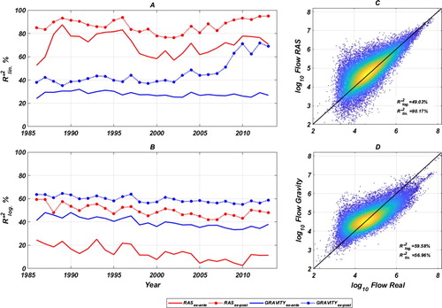
In relative terms (Figure 1(B)), GM generates lower percentage errors than RAS, with values of $R_{log}^2$ around 60% in the ‘ex-post’ aggregation and around 40% in the ‘ex-ante’ aggregation. Overall, the performances in the logarithmic scale result stable over time, although worse than those computed in linear terms. To explain these results, we show the density plot (Figure 1(C)) of the estimations for all the years pooled together, from RAS (panel C) and GM (panel D). In case of little flows, a small relative error implies a small absolute error; while in case of large volumes, a small relative error implies remarkable absolute errors. As a consequence, the failure of GM in ensuring the balance constraints is due to the absolute difference between the estimated and the real large flows ($>{10}^6$ USD), which are systematically below the black line. On the contrary, the RAS algorithm provides accurate estimates of the largest flows (Figure 1(C)) as it guarantees a full closure of the national and global constraints. However, it generates a more spread distribution of estimations of little flows ($<{10}^5$ USD) which explains its lower accuracy in terms of $R_{log}^2$.

Similar results are found when we apply the virtual water weight where slightly lower average values of $R_{lin}^2$ are found as well as slightly higher average values of $R_{log}^2$, with both methodologies (see Figure SM1.1 in SM.1). In this case the GM captured only about the 40% of the real global flow.¹³ This confirms that our procedure can be extended to any other type commodity traded internationally and to other types of networks. These outcomes suggest two take-home messages: first, the aggregative criteria substantially affect the estimative accuracy, with far better performances in case of the ‘ex-post’ procedure. Second, differentiating between absolute and relative errors is crucial to highlight the failure of local balance constraints by the GM, that implies a misleading representation of the real network structure and size. This latter concern has been, more often than not, neglected in the existing studies based on the Gravity Model.

4.2. Topological reconstruction

Figure 2 compares the performances of the GM and RAS in the topology reconstruction (Section 3.3) only based on the ‘ex-post’ aggregation that ensures higher estimative accuracy (see Section 4.1). Panel A shows the share of actual global flow captured by the predicted topology: RAS recovers more than the 95% of the actual bilateral flows under the two different thresholds ($F95\mathrm{\%}$ and $F99\mathrm{\%}$), while the GM is less effective with percentages around 70–80%. Note that the threshold imposes the criterion to define which links must be selected from the estimated topology. However, the estimated bilateral flow might differ from the real ones even when the existence of a link is correctly predicted. This explains the gap between the percentage of total flow imposed by the threshold and the share of actual global flow captured by the two methodologies.

Figure 2. Time series of the estimated network topology performances. Comparison of different simulations (F95% and F99% for RAS, F90% and F95% for GM) from the RAS (red lines) and the GM (blue lines) on the ‘ex-post’ aggregate monetary network. Panels report the real percentage of global flow that lies on the estimated network (A), the percentage of missed links (B), the estimated and real (solid black line) number of links (C), and the percentage of spurious links (D).

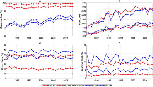
Panel B shows that both RAS (under $F95\mathrm{\%}$) and the GM (under $F90\mathrm{\%}$) define an architecture with a number of links strictly close to the real network (black line). This suggests that there is a trade-off between the total volume that one wants preserve and the total number of connections. However, an efficient combination of the two desiderata can be found in both cases – RAS (under $F95\mathrm{\%}$) and GM (under $F90\mathrm{\%}$) – although RAS recovers a higher share of real flow. Panels C and D offer additional information about the distribution of the estimated links, based on the share of missed (false negative) and spurious (false positive) links. Again, RAS appears to provide better results than the GM. In both cases, independently of the thresholds, the shares of missed links (in the range 20–50%) is higher than the share of connections spuriously added to the real network (in the range 2–8%). Given the high share of global flow captured, this confirms that the IFTN is characterised by a fat-tail distribution where almost all of the trade is concentrated in few big connections. Note that, for both methodologies, a larger number of missed links implies a smaller number of spurious links: a higher threshold reduces the share of missed links, namely the model captures a larger portion of real links, at the cost of greater number of spurious ones. These outcomes confirm that a balanced solution – in terms of false positives and negatives – can be found, again, for RAS under $F95\mathrm{\%}$ and for the GM under $F90\mathrm{\%}$.

Figure 3 provides a graphical representation of the effectiveness of the two methodologies (balanced solutions) to recover the real aggregated network (of the five crops measured in monetary terms) architecture in 2013, although the same messages can be drawn from any other year. For the sake of clarity, links carrying a flow lower than $200,000 U.S. are excluded in order to show only the main bilateral relationships (658 links), which represent around the 31% of the total (2125 links). The color and the thickness of each link are proportional to the traded monetary flow; the node size is proportional to the total node degree (total number of connections) of each country.

Figure 3. Topological reconstruction of the aggregate network topology in monetary terms. Comparison of (A) the real network representing the overall international trade of wheat, rice, maize, soy-bean, and barley summed-up in year 2013, (B) the topological reconstruction based on RAS algorithm, and (C) on the Gravity Model. Flows lower than 200000 USD (0.2 M$) are excluded.

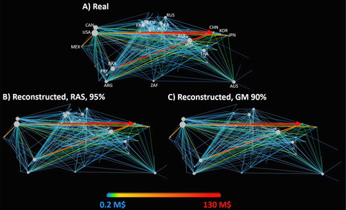
The largest flows are carried along the US–China connection (135 M$), the Brazil–China link (85 M$), and the US–Mexico link (41 M$). Both RAS and GM accurately capture the most important links, and this is also confirmed by the node size of the most central countries (e.g. the US, Mexico, Argentina, Brazil, India, China) that remains the same in both reconstructions. This entails that the predictive power of both methodologies is sufficiently high to capture the real connections of the leading countries, which constitutes the core of the network. Indeed, the average (over the whole time window) backbone index (see Section 3.3), from RAS is 78.6% which is extremely close to the 80% which constitute the real backbone. In case of GM the value is lower, of about 73%. As stated above, both methodologies produce missed and spurious links. In particular, the RAS is able to reconstruct 1087 real links (51%) and the GM is able to reconstruct 922 (43%). From panel C it is clear that the GM tends to miss most of the links in the Mediterranean area, both within Europe and between Europe and Northern Africa. Also the RAS seems to show the largest weaknesses in the topology reconstruction in the European and MENA regions, probably because this area is characterized by many medium-little flows.

5. Discussion

Before moving to the main conclusions it is worth to compare some peculiarities and caveats of the two methods applied in this study which can be resumed in what follows:

1. data requirements: RAS has an advantage in terms of computational cost and data requirements because this algorithm can be successfully applied to recover the bilateral flow intensity simply knowing the aggregate volumes of a given year. On the other hand, the GM needs a series of years to provide a consistent estimation of the coefficients. However, the main difference between these tools is that GM can provide estimates even in absence of trade data (by using country-specific variables, such as GPD, population and so on), while RAS needs at least the total exports and imports;

2. balance constraints: any study related to the problem of flow intensity estimation should explicitly assess the coherence of the regressive model with real data. Indeed, if RAS respects the global and national balance constraints by definition, while the GM systematically underestimates the global flow and national aggregates (i.e. total country's import and export). The latter bias can be overcome with the application of a coefficient of correction, but this caveat can not be overlooked when the GM has to be applied;

3. lack of data: although international trade is a topic that is attracting more attention and it is on the top of the global political agenda, the data availability and reliability of the existing dataset is not guaranteed. Hence, the possibility to recover the structure of the system with a minimum amount of information is of foremost importance to extend the current database to include more remote years. This study proposes a procedure to recover the topology, and then to build new databases, when only aggregate values are available. Both RAS and GM proved to be effective;

4. aggregation bias: the issue of data building is often neglected in the empirical studies. Here, we proved how the criteria used to aggregate more layers (i.e. more commodities) might determine remarkable bias. In general, the application of estimative methods before the aggregative process (i.e. ‘ex-post sum-up’) is proved to be more accurate;

5. scale of analysis: the topological reconstruction obtained from the (‘ex-post’) aggregated networks is more reliable than at single crop-layer scale. This might suggest that some single-level biases tend to cancel-out during the aggregative procedure, partly because the aggregate network is more dense (i.e. more links).

6. Conclusion

In this study we critically assess the estimative accuracy and the predictive power of the RAS algorithm and the gravity model (GM). We also propose a simple, efficient, and generalisable procedure to recover the topology of any network, especially when a low amount of information is available (e.g. total countries' exports and imports). The main outcomes and novelties of the current study can be summarised as:

1. the RAS algorithm generates better performances than the GM when the same regressors are considered;

2. RAS accurately estimates bigger flows ($R_{lin}^2$ high), while GM generates lower errors in relative (percentage) terms ($R_{log}^2$ high);

3. the GM, differently from RAS, does not respect the global balance constraint with systematic under-estimation of the global flow ($F_{tot}$) and then its formulation needs to be corrected with a (row-type) multiplicative factor;

4. both RAS and GM can be applied to recover the network architecture, with a minimum amount of information. However, they have to be calibrated to find an optimal balance between the number of links and the total flow;

5. the application of alternative unit of measures and the extension of different scales, provides a robustness check that allows to the proposed procedure to be generalised to any other type of international trade market.

This study addressed two key issues that are at the core of the current research on international trade: trade flow intensity estimations and link prediction. The former is necessary to understand the strength and the evolution of bilateral trade relationships. Indeed, the underestimation of the overall global flow, as generated by the GM, might lead to misleading results and biased scenarios, mostly when the international trade is tied with the exploitation of natural resources (such as water). This issue is of foremost importance in case of forecasting the evolution of a network, for a proper systemic-risk assessment, and scenario analysis to support policy decisions. Robustness to different scales and unit of measures, should represent a solid base where to found reasonable scenarios to support policy decisions.

To conclude, although this study is empirical in the methods, it offers a solid base for further theoretical research questions (e.g. what is the economic reason behind the systematic under-estimation of the global flow in case of GM? how to interpret the RAS coefficients in an international trade context?) and most of all to understand the reliability of existing estimations and dataset to support policy decision.

Acknowledgments

Thanks are due to Stefania Tamea and Giuseppe Zaccaria for providing us the data on bilateral trade. We acknowledge prof. Marco Diana for early reasoning about the RAS algorithm. Data and results of our work are freely available at https://zenodo.org/record/2863876#.XdaPI1dKhPZ (doi:10.5281/zenodo.2863876).

Disclosure statement

No potential conflict of interest was reported by the authors.

Additional information

Funding

Authors acknowledge European Research Council (ERC) funding for the project: Coping with water scarcity in a globalized world (ERC-2014-CoG, project 647473).

Notes

1 Virtual water refers to the total amount of water that is used in the overall supply chain, from producer to consumer. For a description of the concept see Allan (1993).

2 FAO, Statistics Division. FAOSTAT online database. Available at http://www.fao.org/faostat/en. Last Update on December 11, 2015.

3 The number of active countries changed over time due to political reasons. For example, the USSR is active only until 1991.

4 Note that we clear the series of prices from inflationary effects by tacking real values with base year 2005. Deflators were also provided by FAOSTAT (see http://www.fao.org/faostat/en/#data/PD for further details).

5 We repeat the same procedure in the virtual water obtaining $\mathbf{W}=\mathrm{diag}(\omega )\cdot \mathbf{F}$, where ω is the vector of water intensity coefficient for each country-commodity pair.

6 The use of physical amounts avoids the possible distortion from monetary transformation (e.g. inflation, different currencies and so on).

7 For the sake of completeness, we ran more extensive model including socio-economic factors (e.g. GDP and population size) with no significant improvements of the estimative power.

8 Note that, in the first step, our procedure for the flow intensity estimation excluded the zeros a priori. In this case the log-linear OLS can be considered a benchmark. Moreover, the proposed country-specific OLS regressions generate estimations consistent with real data and with a high goodness of fit.

9 Note that an import-side regression might be calibrated to describe the trade flows entering a given country (Tuninetti et al., 2017); however, it has been proved that the export-side regression outperforms the import law by showing higher coefficients of determination (Tamea et al., 2014; Abdelkader et al., 2018).

10 However, although the absolute levels of the elements of R and S change, their relative values within each vector do not, independently from any initial value (Lahr and De Mesnard, 2004).

11 This expression can be considered as a restricted version of Equation 2(2) $F_{j,k}(t)={\beta }_{0,j}\cdot M_k(t{)}^{{\beta }_{1,j}}\cdot d_{j,k}^{{\beta }_{2,j}},$(2) where each coefficient is 0 with the exception of ${\beta }_2=-1$. Note that, for the sake of completeness, we also applied the GM and RAS in sequence, to say using the Gravity Equation 2(2) $F_{j,k}(t)={\beta }_{0,j}\cdot M_k(t{)}^{{\beta }_{1,j}}\cdot d_{j,k}^{{\beta }_{2,j}},$(2) to estimate the initial conditions. Since the results where not significantly different we opted to keep them separated.

12 In our case we do not consider alternative algorithms because, having complete information, RAS is demonstrated to be an easy and efficient bi-proportional algorithm. See Lenzen et al. (2009) for a review of alternative methods in case of conflicting information.

13 These differences are be due to the distortion that one imposes when adopting different unit of measures. For instance, if virtual water is more stable over time, the monetary conversion is affected by remarkable temporal and spatial variability of food prices (e.g. Distefano et al., 2019).

References

- Abdelkader, A., A. Elshorbagy, M. Tuninetti, F. Laio, L. Ridolfi, H. Fahmy and A.Y. Hoekstra (2018) National Water, Food, and Trade Modeling Framework: The Case of Egypt. Science of the Total Environment, 639, 485–496. doi: 10.1016/j.scitotenv.2018.05.197
- Ahmed, S.A., P.V. Preckel, et al. (2007) A Comparison of RAS and Entropy Methods in Updating IO Tables. 2007 Annual Meeting, Portland, Oregon (US), American Agricultural Economics Association, 1–20.
- Allan, J.A. (1993) Fortunately there are Substitutes for Water Otherwise Our Hydro-political Futures Would Be Impossible. Priorities for Water Resources Allocation and Management, 13, 26.
- Anderson, J.E. (1979) A Theoretical Foundation for the Gravity Equation. The American Economic Review, 69, 106–116.
- Anderson, J.E., M. Vesselovsky and Y.V. Yotov (2016) Gravity with Scale Effects. Journal of International Economics, 100, 174–193. doi: 10.1016/j.jinteco.2016.03.003
- Babiker, M.H. (2005) Climate Change Policy, Market Structure, and Carbon Leakage. Journal of International Economics, 65, 421–445. doi: 10.1016/j.jinteco.2004.01.003
- Balistreri, E.J. and R.H. Hillberry (2008) The Gravity Model: An Illustration of Structural Estimation As Calibration. Economic Inquiry, 46, 511–527. doi: 10.1111/j.1465-7295.2007.00093.x
- Ball, R.J. (1967) An Econometric Study of International Trade Flows. The Economic Journal, 77, 366–368. doi: 10.2307/2229319
- Bergstrand, J.H. (1985) The Gravity Equation in International Trade: Some Microeconomic Foundations and Empirical Evidence. The Review of Economics and Statistics, 67, 474–481. doi: 10.2307/1925976
- Blum, B.S. and A. Goldfarb (2006) Does the Internet Defy the Law of Gravity? Journal of International Economics, 70, 384–405. doi: 10.1016/j.jinteco.2005.10.002
- Bon, R. (1984) Comparative Stability Analysis of Multiregional Input–output Models: Column, Row, and Leontief-strout Gravity Coefficient Models. The Quarterly Journal of Economics, 99, 791–815. doi: 10.2307/1883126
- Bregman, L.M. (1967) Proof of the Convergence of Sheleikhovskii's Method for a Problem with Transportation Constraints. USSR Computational Mathematics and Mathematical Physics, 7, 191–204. doi: 10.1016/0041-5553(67)90069-9
- Chaney, T. (2018) The Gravity Equation in International Trade: An Explanation. Journal of Political Economy, 126, 150–177. doi: 10.1086/694292
- D'Alessandro, S., T. Distefano, A. Cieplinski and K. Dittmer (2018) EUROGREEN Model of Job Creation in a Post-Growth Economy. Type Tech Report. EUROGREEN Project. https://people.unipi.it/simone_dalessandro/wp-content/uploads/sites/78/2018/10/EUROGREEN_Project.pdf.
- D'Odorico, P., J.A. Carr, F. Laio, L. Ridolfi and S. Vandoni (2014) Feeding Humanity Through Global Food Trade. Earth's Future, 2, 458–469. doi:10.1002/2014EF000250
- Dell'Angelo, J., P. D'Odorico and M.C. Rulli (2017) Threats to Sustainable Development Posed by Land and Water Grabbing. Current Opinion in Environmental Sustainability, 26, 120–128. doi: 10.1016/j.cosust.2017.07.007
- Dietzenbacher, E. and R. Hoekstra (2002) The RAS Structural Decomposition Approach. In: Trade, Networks and Hierarchies. Berlin, Heidelberg, Springer, 179–199.
- Distefano, T., G. Chiarotti, F. Laio and L. Ridolfi (2019) Spatial Distribution of the International Food Prices: Unexpected Heterogeneity and Randomness. Ecological Economics, 159, 122–132. doi:10.1016/j.ecolecon.2019.01.010
- Distefano, T., F. Laio, L. Ridolfi and S. Schiavo (2018a) Shock Transmission in the International Food Trade Network. PLoS One, 13, e0200639. doi:10.1371/journal.pone.0200639
- Distefano, T., M. Riccaboni and G. Marin (2018b) Systemic Risk in the Global Water Input–output Network. Water Resources and Economics, 23, 28–52. doi:10.1016/j.wre.2018.01.004
- Fagiolo, G. (2010) The International-trade Network: Gravity Equations and Topological Properties. Journal of Economic Interaction and Coordination, 5, 1–25. doi: 10.1007/s11403-010-0061-y
- Fagiolo, G., J. Reyes and S. Schiavo (2010) The Evolution of the World Trade Web: a Weighted-network Analysis. Journal of Evolutionary Economics, 20, 479–514. doi: 10.1007/s00191-009-0160-x
- Fally, T. (2015) Structural Gravity and Fixed Effects. Journal of International Economics, 97, 76–85. doi:10.1016/j.jinteco.2015.05.005
- Fracasso, A. (2014) A Gravity Model of Virtual Water Trade. Ecological Economics, 108, 215–228. doi: 10.1016/j.ecolecon.2014.10.010
- Gallego, B. and M. Lenzen (2009) Estimating Generalised Regional Input–Output Systems: A Case Study of Australia. In: The Dynamics of Regions and Networks in Industrial Ecosystems. Boston, MA, Edward Elgar Publishing, 55–82.
- Getoor, L. and C.P. Diehl (2005) Link Mining: a Survey. Acm Sigkdd Explorations Newsletter, 7, 3–12. doi: 10.1145/1117454.1117456
- Giordani, P.E., N. Rocha and M. Ruta (2016) Food Prices and the Multiplier Effect of Trade Policy. Journal of International Economics, 101, 102–122. doi: 10.1016/j.jinteco.2016.04.001
- Huang, Z. and D.K. Lin (2009) The Time-series Link Prediction Problem with Applications in Communication Surveillance. INFORMS Journal on Computing, 21, 286–303. doi: 10.1287/ijoc.1080.0292
- Ivus, O. and A. Strong (2007) Modeling Approaches to the Analysis of Trade Policy: Computable General Equilibrium and Gravity Models. In: William A. Kerr and James D. Gaisford (eds.), Handbook on International Trade Policy. Cheltenham UK, Edward Elgar Publishing, 44.
- Kepaptsoglou, K., M.G. Karlaftis and D. Tsamboulas (2010) The Gravity Model Specification for Modeling International Trade Flows and Free Trade Agreement Effects: a 10-year Review of Empirical Studies. The Open Economics Journal, 3, 1–13. doi: 10.2174/1874919401003010001
- Konar, M., C. Dalin, S. Suweis, N. Hanasaki, A. Rinaldo and I. Rodriguez-Iturbe (2011) Water for Food: The Global Virtual Water Trade Network. Water Resources Research, 47, W05520. doi:10.1029/2010WR010307
- Krugman, P. (1980) Scale Economies, Product Differentiation, and the Pattern of Trade. The American Economic Review, 70, 950–959.
- Lahr, M. and L. De Mesnard (2004) Biproportional Techniques in Input–output Analysis: Table Updating and Structural Analysis. Economic Systems Research, 16, 115–134. doi: 10.1080/0953531042000219259
- Ledwoch, A., H. Yasarcan and A. Brintrup (2018) The Moderating Impact of Supply Network Topology on the Effectiveness of Risk Management. International Journal of Production Economics, 197, 13–26. doi: 10.1016/j.ijpe.2017.12.013
- Lenzen, M., B. Gallego and R. Wood (2009) Matrix Balancing Under Conflicting Information. Economic Systems Research, 21, 23–44. doi: 10.1080/09535310802688661
- Lenzen, M., D. Moran, K. Kanemoto and A. Geschke (2013) Building Eora: a Global Multi-region Input–output Database At High Country and Sector Resolution. Economic Systems Research, 25, 20–49. doi: 10.1080/09535314.2013.769938
- McDougall, R.A. (1999) Entropy Theory and RAS are Friends, GTAP Working Papers 300, Center for Global Trade Analysis, Department of Agricultural Economics, Purdue University, USA. http://docs.lib.purdue.edu/gtapwp/6
- Moon, B.E. (2018) Dilemmas of International Trade. New York: Routledge.
- Niepmann, F. and T. Schmidt-Eisenlohr (2017) International Trade, Risk and the Role of Banks. Journal of International Economics, 107, 111–126. doi: 10.1016/j.jinteco.2017.03.007
- Overman, H.G., S. Redding and A.J. Venables (2001) The Economic Geography of Trade, Production, and Income: A Survey of Empirics. In: William A. Kerr and James D. Gaisford (eds.), Handbook of International Trade. Cheltenham UK, Edward Elgar Publishing, 350–387.
- Pinilla, V., R. Duarte and A. Serrano (2018) Factors Driving Embodied Carbon in International Trade: A Multiregional Input–Output Gravity Model. Economic Systems Research, 30, 545–566. doi:10.1080/09535314.2018.1450226
- Robinson, S., A. Cattaneo and M. El-Said (2001) Updating and Estimating a Social Accounting Matrix Using Cross Entropy Methods. Economic Systems Research, 13, 47–64. doi: 10.1080/09535310120026247
- Sargento, A.L., P.N. Ramos and G.J. Hewings (2012) Inter-regional Trade Flow Estimation Through Non-survey Models: An Empirical Assessment. Economic Systems Research, 24, 173–193. doi: 10.1080/09535314.2011.574609
- Sarker, R. and S. Jayasinghe (2007) Regional Trade Agreements and Trade in Agri-food Products: Evidence for the European Union From Gravity Modeling Using Disaggregated Data. Agricultural Economics, 37, 93–104. doi: 10.1111/j.1574-0862.2007.00227.x
- Schneider, M. and S. Zenios (1990) A Comparative Study of Algorithms for Matrix Balancing. Operations Research, 38, 439–455. doi: 10.1287/opre.38.3.439
- Serrano, M.A. and M. Boguñá (2003) Topology of the World Trade Web. Physical Review E, 68, 015101. doi:10.1103/PhysRevE.68.015101
- Tamea, S., J. Carr, F. Laio and L. Ridolfi (2014) Drivers of the Virtual Water Trade. Water Resources Research, 50, 17–28. doi: 10.1002/2013WR014707
- Tarancón, M.Á. and P.D. Rio (2005) Projection of Input–Output Tables by Means of Mathematical Programming Based on the Hypothesis of Stable Structural Evolution. Economic Systems Research, 17, 1–23. doi: 10.1080/09535310500034119
- Toh, M.H. (1998) The RAS Approach in Updating Input–Output Matrices: An Instrumental Variable Interpretation and Analysis of Structural Change. Economic Systems Research, 10, 63–78. doi: 10.1080/09535319800000006
- Tuninetti, M., S. Tamea, F. Laio and L. Ridolfi (2017) To Trade Or Not to Trade: Link Prediction in the Virtual Water Network. Advances in Water Resources, 110, 528–537. doi: 10.1016/j.advwatres.2016.08.013
- Vidmer, A., A. Zeng, M. Medo and Y.C. Zhang (2015) Prediction in Complex Systems: The Case of the International Trade Network. Physica A: Statistical Mechanics and its Applications, 436, 188–199. doi: 10.1016/j.physa.2015.05.057
- White, D.J., K. Hubacek, K. Feng, L. Sun and B. Meng (2018) The Water-energy-food Nexus in East Asia: A Tele-connected Value Chain Analysis Using Inter-regional Input-Output Analysis. Applied Energy, 210, 550–567. doi: 10.1016/j.apenergy.2017.05.159
- Wiebe, K.S. and M. Lenzen (2016) To RAS Or Not to RAS? What is the Difference in Outcomes in Multi-regional Input–Output Models? Economic Systems Research, 28, 383–402. doi: 10.1080/09535314.2016.1192528