Systemic risk and macro-financial interconnectedness using an FSAM framework

Abstract

We provide a general framework to assess the traceability of systemic risk and macro interconnectedness to understand the financial risk transmissions channels. Our contribution help address the information need established in the DGI-2 in a FSAM-based model that fully captures the interconnectedness between real and financial sectors. Recent developments in the field of IO and SAM evaluations have led to a renewed interest in the usage of linkage analysis to measure the role that a sector play within the economy. Focusing on the backward and forward linkage, hypothetical extraction method, and structural path analysis, we show how feasible it is to include heterogeneous financial institutions to study risk interactions effects on macroeconomic outcomes. This paper’s proposal may be useful for thinking about how micro-data and macro-aggregates can be incorporated into the set of financial soundness indicators, allowing to obtain an idea of the vulnerabilities of the financial sector.

KEYWORDS:

• Financial Social Accounting Matrix
• interlinkages
• structural path analysis
• hypothetical extraction method
• fixed-price multiplier model

1. Introduction

The nexus between real and financial activity has been the focus of the discussions following the Global Financial Crisis (GFC). The main lesson learned has been the need to understand the intricated links between macroeconomic conditions and the systemic risks embedded in the financial systems. Although the general economic conditions (production, investment, consumption, and so forth) are relevant factors to explain systemic risk at a sectoral level (Demirgüç-Kunt & Levine, 2018), little attention has been given to the risk interactions between financial institutions and non-financial sectors (credit or counterparty risk) due to many and complex relationships that take place among them (Bremus et al., 2018).¹

In the wake of the 2008 financial and economic crisis, the Group of Twenty economies (G-20) asked the Financial Stability Board (FSB) and International Monetary Fund (IMF) to explore gaps and provide appropriate proposals for strengthening data collection before the next meeting of the G-20′s Finance Ministers and Central Bank Governors. In April 2009, the FSB-IMF came up with 20 recommendations, known now as the Data Gaps Initiative (DGI-1), to address information gaps revealed by the global financial crisis. In September 2015, the FSB-IMF concluded the first initiative and started a second phase (DGI-2). The DGI-2 recommendations maintain the continuity of DGI-1; however, they claim that more focus is needed on data sets that support the monitoring of risks in the financial sector and the analysis of the interlinkages across economic and in particular in the financial system (IMF & FSB, 2015).

The second stage of the G20 initiative has emphasized the need to deeply monitor financial risks (credit, market, liquidity, for example), as well as the analysis of inter-linkages and spillovers in the financial sector. Despite the current progress in closing and identifying data gaps, there is a high consensus that further steps need to be taken to bring the relevant information foundation to a satisfactory level, particularly for micro-level data (Bremus & Buch, 2017; Kasinger & Pelizzon, 2018).

The participating economies have made significant progress during the second phase of the DGI-2 implementation (FSB, 2018). Nevertheless, key challenges remain, which hamper the implementation of some of the FSB-IMF recommendations. In the like manner, the Inter-Agency Group on Economic and Financial Statistics (IAG)² has underlined that a macro-financial linkage has two requirements. First, to help assess the various means by which shocks to the financial sector can result in a feedback loop to the real sectors, which includes understanding the contagion effects within the financial sector. Second, allow monitoring macroeconomic conditions and impacts of significant shocks into the economy.

Our main contribution relies on developing an applied framework for policy analysis of macro-micro financial linkages, focused on five of the DGI-2 recommendations embedded in an financial social accounting matrix (FSAM)-based model that fully captures the interconnectedness between the real and financial sectors of an economy.³

Information contained in a social accounting matrix (SAM) (e.g. input coefficients matrix) results actually in a snapshot of economic interconnections among sectors in an economy at a given point in time (Miller & Lahr, 2001). The SAM system provides a relevant framework to model risk in both financial and non-financial sector in terms of their sensitivity to shocks generated in the macroeconomic environment or the financial markets. Therefore, a SAM system, considering aggregated and disaggregated industry levels within a FSAM multiplier, allow identifying how capital and financial linkages influence the economic policy interactions (Achjar et al., 2006; Aray et al., 2017; Bezemer, 2010; Emini & Fofack, 2004; Roland-Holst & Sancho, 1995; Tsujimura & Tsujimura, 2010).

However, the multipliers analysis alone cannot clarify the structural and behavioral mechanism (or black box) resulting in the accounting multipliers (Thorbecke, 2000). From a policy standpoint, it becomes more relevant to unveil the network of financial and real paths along which a shock travels through the economy. Understanding risk determinants and channels of risk transmission of macro-financial shocks is relevant for policy and financial crisis management.

Authors like Lima and Drumond (2016) and Heath and Goksu (2017) have emphasized the need to monitor particular financial institutions with strong linkages between institutions, and therefore, assess the connections between those financial and non-financial corporations. In this vein, numerous studies have attempted to explain that a holistic approach to financial stability analysis helps straddle the gap between micro and macro analysis (Heath & Goksu, 2016; Saldías, 2011; Tissot, 2016). Therefore, micro- and macroprudential analysts need both macro-aggregates and granular data (micro-data) to enhance the accuracy and level of traditional economic analysis details. Combining these two sources of information, policymakers can better identify, measure, and monitor, on an ongoing basis, the risk profiles embedded in structured credit products and credit risk transfer instruments (IMF & FSB, 2019).

Dealing with appropriate methodological requirements, this research show how feasible it is to include individual banks’ information into the FSAM, keeping the inherent accounting rules and ensuring the balances are satisfied. In particular, the availability of micro-data and links between the macro (macro-aggregates) and micro (micro-data) becomes crucial for macroprudential policy, given the importance of focusing on the links mentioned across financial institutions and between them and the non-financial institutions. Extending the macro-financial linkages analysis through an FSAM multiplier results in a decision-making tool to analyze systemic risks originated in the financial sector. It provides a consistent accounting framework about the financial sector and the structure of an economy as a whole. It is also a valuable tool for understanding the macro-financial linkages of an economy (Aray et al., 2017).

This paper has been organized in the following way. The next section deals with the theoretical FSAM framework. It shows how to allocate micro and macro data on the financial sector into an accounting scheme in the case of a fully decomposed financial sector. The third section is concerned with the simulation methodology used for this study. Here, we present the approaches commonly applied to measure interindustry linkages and the importance of industries for measuring the role of a sector in the economy. These are the Backward and Forward linkage analysis (BFL), the linkage analysis based on a hypothetical extraction method (HEM), and the structural path analysis (SPA). The fourth section presents the simulation results, focusing on capturing the interconnectedness between real and financial sectors. Finally, Section 5 presents the conclusions and final considerations.

2. Theoretical framework

2.1. The financial social accounting matrix

A SAM is a square matrix $\mathbf{T}$ of monetary flows designed to provide a record of transactions using a single-entry form of bookkeeping. It can be represented as (Pyatt, 1988): (1) $\begin{array}{r}\mathbf{T}=[t_{ij}]\end{array}$(1) where $i$ is the number of row transaction, $j$ the number of the column transaction, and the total number of transactions, called accounts, constitutes the dimension of the square matrix. By convention, all row accounts represent incomes (resources), while the column accounts represent expenditures (uses). Therefore, $t_{ij}$ shows the transaction value where the income obtained by account $i$ originates from the expenditure by account $j$ during an accounting period. In this sense, a SAM results in an extension of the input-output (IO) accounts that trace out the circular income flow, including production activities, commodities, factors, domestic institutional sector – households, enterprises and government – and the rest of the world.

Depending on how the accounts are defined, including their analytical interest and specific policy concern, the classification of accounts in a social accounting matrix can assume diverse forms. As Hubic (2012) has pointed out, a social accounting matrix can be classified as a real SAM and an FSAM. The first records only the transactions of the economic institutions’ real activities. The second presents the complete circular flow of funds within the economy's real side and the transactions across the financial system. Therefore, the FSAM framework represents an essential extension to the IO models since it fully captures the interconnectedness between the real and financial sectors of an economy (Aray et al., 2017).

In this sense, the FSAM used in this research use six major types of endogenous accounts: i) production by commodities, ii) output by activities, iii) income generation, iv) income distribution, v) capital account, and vi) financial account⁴. The accounting scheme is based on the FSAM developed by Aray et al. (2017) for Spain, and the discussion on each account is presented below: (2) $\begin{array}{r}{\mathbf{T}}_{\text{FSAM}}=\left[\begin{array}{cccccccc}0& \mathbf{I}{\mathbf{C}}_{m\times m}& 0& 0& {\mathbf{C}}_{m\times k}& 0& {\mathbf{K}}_{m\times g}& 0\\ {\mathbf{O}}_{m\times \mathrm{m}}& 0& 0& 0& 0& 0& 0& 0\\ 0& \mathbf{V}{\mathbf{A}}_{k\times m}& 0& 0& 0& 0& 0& 0\\ 0& 0& {\mathbf{V}\mathbf{A}}_{p\times k}^{\ast }& \mathbf{P}{\mathbf{I}}_{p\times p}& 0& 0& 0& 0\\ 0& 0& 0& {\mathbf{C}}_{p\times p}^{\ast }& 0& 0& 0& 0\\ 0& 0& 0& {\mathbf{S}}_{p\times p}& 0& \mathbf{K}{\mathbf{T}}_{p\times p}& 0& \mathbf{F}{\mathbf{L}}_{p\times q}\\ 0& 0& 0& 0& 0& {{\mathbf{K}}^{\ast }}_{g\times p}& 0& 0\\ 0& 0& 0& 0& 0& \mathbf{F}{\mathbf{A}}_{q\times p}& 0& 0\end{array}\right]\end{array}$(2) From this set of linear equations, ${\mathbf{T}}_{\text{FSAM}}$ constitute a sequence of accounts that begins with the real economy sphere (IO framework), by recording the output in the production matrix (${\mathbf{O}}_{m\times \mathrm{m}}$), the input of the intermediate consumption matrix ($\mathbf{I}{\mathbf{C}}_{m\times m}$), and leave the value-added ($\mathbf{V}{\mathbf{A}}_{k\times m}$) as the matrix balancing item⁵. The generation of income and distribution (SAM framework) describes how production factors (such as labor and capital) generate income and transfer it to their institutional sector (${\mathbf{V}\mathbf{A}}_{p\times k}^{\ast }$). Simultaneously, value added is augmented by property income ($\mathbf{P}{\mathbf{I}}_{p\times p}$), which collects the accrued income because the owners of financial assets and natural resources have put them at the disposal of other institutional sectors (dividends and interests).⁶ Besides, each institutional sector allocates its disposable income between final consumption expenditures (${\mathbf{C}}_{p\times p}^{\ast }$) and saving (${\mathbf{S}}_{p\times p}$). Where the final-demand expenditure for products made by households, NPISHs and the government is recorded in the final consumption matrix ${\mathbf{C}}_{m\times p}$, and by the accumulation account by products and type of non-financial assets recorded in the gross capital formation matrix ${\mathbf{K}}_{m\times g}$. Finally, the financial interconnectedness with the real sector of the economy is recorded by institutional sectors (FSAM framework): saving, net capital transfer ($\mathbf{K}{\mathbf{T}}_{p\times p}$) and financial liability flows ($\mathbf{F}{\mathbf{L}}_{p\times q}$), which are used to acquire non-financial assets (${{\mathbf{K}}^{\ast }}_{g\times p}$) and financial asset flows ($\mathbf{F}{\mathbf{A}}_{q\times p}$). In this part of the flow, the net lending/borrowing process represents the balancing item between the capital and financial accounts. The final balancing item of this set of accounts is saving, which is the part of disposable income that is not spent for consumption purposes but used – in addition to any capital transfer – to buy financial assets or to reduce financial liabilities.

The formal framework for analyzing the effects of diverse economic shocks through the information contained in the ${\mathbf{T}}_{\text{FSAM}}$ is a multiplier analysis as proposed by Emini and Fofack (2004), which allows simulating the impact analysis of the linkage between exogenous and endogenous accounts by configuring a fixed-price multiplier model typically specified by the set of equations below: (3) $\begin{array}{r}\mathbf{y}=\mathbf{A}\mathbf{y}+\mathbf{x}=(\mathbf{I}-\mathbf{A}{)}^{-1}\mathbf{x}=\mathbf{M}\mathbf{x}\end{array}$(3) where $\mathbf{y}$ represents a vector of the combined real sector and financial sector endogenous account totals, and $\mathbf{x}$ is a vector of the combined real sector and financial sector exogenous account totals. If $\mathbf{A}\equiv \mathbf{T}(\hat{\mathbf{y}}{)}^{-1}$defines the matrix of average expenditure propensities and is assumed to be fixed, then $\mathbf{M}$ is fixed, where the elements of this matrix, $m_{ij}$, show the increment of the endogenous account, $i$, caused by the increase in one monetary unit of the exogenous account.⁷ In brief, Equation 3 determines the total equilibrium of production, income, final demand (consumption and investment), and the equilibrium in the capital and financial account contained in $\mathbf{y}$, which are consistent with any set of injections,$\mathbf{x}$. In an FSAM framework, the impact multiplier captures the overall effects (direct, indirect and induced) on outputs, income and financial accounts from a unitary and exogenous shock.

In this sense, the real-financial linkage in the economy is traceable through the interactions of saving-investment balances of institutions in the FSAM framework. It is straightforward to note that for each economic sector and also for the whole economy, the following identity always holds: (4) $\begin{array}{r}{\mathbf{s}}_p-{{\mathbf{k}}^{\ast }}_p=\mathbf{f}{\mathbf{a}}_p-\mathbf{f}{\mathbf{l}}_p\end{array}$(4) Equation 4 is the well-known macro-financial relationship of the economy in SNA, in which the balance of savings and investment is equal to the net financial operation, i.e. net lending means that savings surpass investment and net borrowing implies that investments exceed savings (Aray et al., 2017). The role of financial intermediation is one of devising financial instruments ($\mathbf{F}{\mathbf{A}}_{q\times p}$) that encourage those with saving (${\mathbf{S}}_{p\times p}$) to lend these funds to financial institutions, so that these financial institutions, in a second-round, can then lend the same funds to other sectors ($\mathbf{F}{\mathbf{L}}_{p\times q}$), matching the needs of borrowers (${{\mathbf{K}}^{\ast }}_{\mathrm{g}\times p}$) with the desires of lenders between institutional sectors. The financial institutions’ role is the use of the net borrowing funds and their funds to acquire mainly financial assets either by making loans and receiving deposits or by purchasing and issuing bills, bonds, and other securities (United Nations et al., 2008).

The macro-financial interconnectedness encompasses financial risk management (i.e. market and credit risk) and liquidity transformation (assets and liabilities management). As a result, the accounting scheme expressed in the ${\mathbf{T}}_{\text{FSAM}}$ matrix capture broadly the disaggregation of an economy by representing all the monetary transactions occurring within a given period. As noted by van de Ven and Fano (2017), the knowledge of the financial linkages between the economics agents in the economy by capturing the flows between different sectors results in an outstanding analytical tool in macroeconomic and financial areas for macro-stability analysis.

2.2. Allocation of financial intermediation services from financial institutions by industries

To deepen the role that financial intermediation services play, we must understand the characteristics that distinguish financial institutions in the real sector economy. Under the International Standard Industrial Classification of all economic activities (ISIC, Rev.4), corporations are classified into industries according to the type of goods and services they are mainly involved in producing, and not by their ultimate ownership (Burgess, 2011). In this regard, corporations are divided between those resident institutional units, mainly providing financial services and those offering goods and other services. In the case of financial services, these are financial intermediaries, which typically comprise a significant part of financial services and require stringent supervision to provide these services (United Nations et al., 2008).⁸

According to the ISIC definition, we identify two groups of industries or blocks in the economy, first, those whose principal activity is the production of goods or non-financial services, denoted by the superscripts $\text{N}$, and second, those who are engaged in providing financial services, denoted by the superscripts $\text{F}$. Thus, the submatrix $\mathbf{I}{\mathbf{C}}_{m\times m}$ of intermediate consumption from ${\mathbf{T}}_{\text{FSAM}}$ in Equation 2 can be expanded as: (5) $\begin{array}{r}\mathbf{I}\mathbf{C}=\left[\begin{array}{cc}\mathbf{I}{\mathbf{C}}^{\mathrm{N}-\mathrm{N}}& \mathbf{I}{\mathbf{C}}^{\mathrm{N}-\mathrm{F}}\\ \mathbf{I}{\mathbf{C}}^{\mathrm{F}-\mathrm{N}}& \mathbf{I}{\mathbf{C}}^{\mathrm{F}-\mathrm{F}}\end{array}\right]\end{array}$(5) If we define $n$ heterogeneous financial institutions, the submatrices $\mathbf{I}{\mathbf{C}}^{\mathrm{N}-\mathrm{N}}$ and $\mathbf{I}{\mathbf{C}}^{\mathrm{F}-\mathrm{F}}$ are defined as square matrices of size $(m-1)\times (m-1)$ and$n\times n$, respectively. The sizes of $\mathbf{I}{\mathbf{C}}^{\mathrm{N}-\mathrm{F}}$and $\mathbf{I}{\mathbf{C}}^{\mathrm{F}-\mathrm{N}}$, therefore, are $(m-1)\times n$ and $n\times (m-1)$, respectively.

Throughout this research, when referring to sectoral economic activities, we are going to make explicit the distinction between non-financial corporations and financial institutions. For analytical purposes, when implementing ISIC at its lower levels of detail, we can observe and analyze the economic interactions among different activities and $n$ heterogeneous financial institutions. It allows understanding the interlinkages of the production into an economy (United Nations et al., 2008).

As can be noticed, matrices $\mathbf{I}{\mathbf{C}}^{\mathrm{N}-\mathrm{N}}$ and $\mathbf{I}{\mathbf{C}}^{\mathrm{N}-\mathrm{F}}$ in Equation 5 correspond that component of the accounting flow matrices of intermediate consumption, holding the monetary value of market goods and non-financial services consumed or used up as inputs in production by firms. The first matrix shows the aggregate intermediate consumption accounted by $(m-1)$ non-financial corporations grouped by industries (macro-level). The second matrix holds the disaggregated intermediate consumption of the goods market and non-financial services consumed by $n$financial institutions (micro-level).

Similarly, the matrix $\mathbf{I}{\mathbf{C}}^{\mathrm{F}-\mathrm{F}}$ refers to the net account flow matrix of interbank financial intermediation between $n$ financial institutions, and matrix $\mathbf{I}{\mathbf{C}}^{\mathrm{F}-\mathrm{N}}$ captures the flow of financial services of intermediation consumption used by non-financial corporations from financial institutions. Note that the last submatrix record all payable fees the payment for the provision of financial intermediation services breakdowns hold by the real sector economic activities from $n$financial institutions in the real economy.

As the last financial crisis revealed, the classification of lending and funding by industries provides insights into banks’ liquidity and credit risk exposures (IMF & FSB, 2009). Making explicit the sub-matrix $\mathbf{I}{\mathbf{C}}^{\mathrm{F}-\mathrm{N}}$ comprises micro-level information of the financial services provided in association with explicit fees charges instead of providing services (credits and deposits), transactions in foreign currencies, and implicit fees from financial intermediation services not measured directly.

2.3. Allocating microdata from the financial sector into a SAM framework

The information needed to calculate the submatrix $\mathbf{I}{\mathbf{C}}_{m\times m}$ of intermediate consumption, as proposed in Equation 5 by industry, is unlikely to be available at the bank level. In fact, as has been pointed out by the Data Gaps Initiative II (IMF & FSB, 2019), information on the value of financial assets and liabilities by local banking office breakdowns by industry are not publicly available in most European countries. Therefore, it may not be feasible to directly compute the intermediate consumption for each establishment of the financial sector using the bottom-up approach. The way to bridge this gap is to follow the guidelines of the SNA (United Nations et al., 2008). In this sense, we will allocate the intermediate consumption of domestically produced by a financial institution to industries using the top-down approach, undertaken bank-level data available at the regional level.

Additionally, we consider a relevant market approach for computing the market share (stocks of credits and deposits) at the regional level (particularly, provinces). Many savings and commercial banks were firms with regional attaching in one or a few provinces. In this respect, authors like Carbó-Valverde and Rodríguez (2004) and Fernandez de Guevara and Maudos (2007) have shown empirically that the relationship between finance and economic growth is likely to be more adequately evaluated in a regional framework within a single country. These authors state that the regional level represents an accurate definition of the relevant retail bank market. All sorts of institutional, legal, and cultural differences may be held constant at the regional level⁹.

Similar to Carbó-Valverde et al. (2003) and Fernandez de Guevara and Maudos (2007), we assume that the average fee value of financial services per branch office in a financial institution: i) is the same for all branch offices of the same financial institution; ii) is the same for all branches at all financial institutions; and iii) is the same over economic activities at all regions. Assumption i) says that the value of credit (or loans), at each branch office of a given financial institution, can be approximated by the ratio of the financial institution’s total deposits (or loans) to its total number of branch offices. Although data limitations preclude us from doing anything about this assumption, we proceed like Carbó-Valverde and Rodríguez (2004) to do something about the other two assumptions.

Given that the available information at the industry-level for each firm is the distribution of its branch office network by region, the expected value of intermediate consumption at bank-level by industry is computed as a weighted average of the values of these variables in the different regions where they operate. We employ the number of branches by bank $n$ in a specific region $r$ according to the weighting factor of the value-added for each economic sectoral activity $m$ in each region $r$: (6) $\begin{array}{r}\text{E}[{\mathbf{I}\mathbf{C}}_{n\times m}^{\mathrm{F}-\mathrm{N}}]={\mathbf{i}\mathbf{c}}_m^{\mathrm{F}-\mathrm{N}}\times \sum _{r=1}^{\text{R}}\left(\frac{V{A}_{m,r}}{V{A}_m}\times \frac{\text{MFIs branche}{\text{s}}_{n,r}}{\text{Branches in province}{\text{s}}_r}\right)+{ϵ}_{n\times m}\end{array}$(6) where ${\mathbf{i}\mathbf{c}}_m^{\mathrm{F}-\mathrm{N}}$ is the vector of intermediate consumption of financial intermediation services breakdowns by each economic sectoral activity $m$ as reported in the IO table,¹⁰ and $ϵ$ is a random-disturbance matrix term assumed with zero mean and constant variance among banks.

This estimation approach lets the value of intermediate consumption per office to vary across banks and over industries, removing assumptions ii) and iii). While IO models are essentially deterministic (Rueda-Cantuche et al., 2013), the technological parameters derived through the expression above may derive an uncertainty bias at the bank level.

The underlying aim to make explicit the error term $ϵ$ is that a miscalculation in one input coefficient may cause larger effects on the fixed-price multiplier matrix than the same error in another input coefficient (Dietzenbacher, 2006). For this reason, to capture the uncertainty effects over the expected value of intermediate consumption at the bank level, this research makes the error term explicit by contrasting the results from expression (6) against the credit exposure disclosed in the Pillar 3 reports found for each financial institution¹¹.

Disclosure requirements have become an integral part of the Basel Committee on Banking Supervision framework (BCBS, 2017a), and financial institutions must publish a standalone document that provides a readily accessible source of prudential measures of credit exposure. However, the available information in the Basel framework raises some caveats. First, the sectoral breakdown does not reach the disaggregation level proposed by this research (ISIC at 2 digit, Rev 4.). The banks’s disclosure Pillar 3 reports are not homogeneously disclosed, making their comparability not entirely achievable among banks. Despite all this, the availability of this meaningful information about risk metrics results fundamental to knowing the soundness of the financial system and allows reducing the uncertainty of the technical coefficients, as has been suggested by Dietzenbacher (2006) and Temursho (2017).¹²

Furthermore, according to the sectoral balances analysis approach (Saldías, 2011), the expected values resulting from expression (6) capture, in fact, the sectoral credit concentration hold by each financial institution allowing monitoring in a specific way the likelihood of a sectoral slump. Thus, the approach here presented are aligned with the idea of granular origins of aggregate fluctuations developed by Gabaix (2011), who established that idiosyncratic firm-level shocks can explain a large part of aggregate movements and provide a microfoundation for aggregate shocks on which this research is based.

In this vein, the empirical results of Blank et al. (2009), Bremus and Buch (2017) and Amiti and Weinstein (2018) are relevant to support our proposal. Their empirical results have shown how idiosyncratic bank shocks allow to understand in part the links between the real and financial sector, and show how granular effects arise if financial markets are very concentrated. Bremus and Buch (2017) show that if a few large banks coexist with many small banks, idiosyncratic shocks to individual banks do not have to cancel out in the aggregate, but can affect macroeconomic fluctuations as this research proposes.

In this sense, results straightforward from expressions (6) that we can assess sectoral risks both from a micro and a macro-prudential perspective by computing two measures of banks’ sectoral credit risk exposure applied in the macro-prudential literature and embedded in the FSAM framework: i) the sectoral credit concentration, ${\rho }_m$, and ii) the Hirschman-Herfindahl Index ($\text{HHI}$), given that: (7) $\begin{array}{r}{\mathbf{I}\mathbf{C}}_{n\times m}^{\text{F}-\text{N}}=\left[\begin{array}{cccc}{\hat{i}}_{11}^{\mathrm{F}-\mathrm{N}}& {\hat{i}}_{12}^{\mathrm{F}-\mathrm{N}}& \cdots & {\hat{i}}_{1m}^{\mathrm{F}-\mathrm{N}}\\ {\hat{i}}_{21}^{\mathrm{F}-\mathrm{N}}& {\hat{i}}_{22}^{\mathrm{F}-\mathrm{N}}& \cdots & ⋮\\ ⋮& ⋮& \ddots & ⋮\\ {\hat{i}}_{n1}^{\mathrm{F}-\mathrm{N}}& {\hat{i}}_{n2}^{\mathrm{F}-\mathrm{N}}& \cdots & {\hat{i}}_{nm}^{\mathrm{F}-\mathrm{N}}\end{array}\right];{\rho }_m=\frac{{\hat{i}}_{nm}^{\mathrm{F}-\mathrm{N}}}{\sum _{m=1}{\hat{i}}_{nm}^{\mathrm{F}-\mathrm{N}}};HHI=\sum _{m=1{\rho }_m^2}\end{array}$(7) By making explicit the results of expression (7), we build an analytical instrument to present information associated with the intermediate consumption composition by each economic sectoral activity $m$ (ISIC-Division) and granular detail of banking institutions (bank $n$) with explicit relationships with both the real and financial dimensions.

The allocation of granular data from the financial sector into an FSAM framework might help micro and macro-prudential authorities to identify the build-up of sectoral risks in individual banks portfolios or within the banking system at large. According to the BCBS (2018) the prerequisite for any effective policy supervision approach is a statistical framework that allows for effective analysis and monitoring of the Global Systemically Important Banks (G-SIB) and Other Systemically Important Institutions (O-SII). Hence, this research allows reducing the information gap regarding the importance of concentration and distributional measures to analyze macro-financial stability as requested by the IMF’s financial surveillance strategy (Borio, 2013).

3. Simulation approach

The importance of a sector within an economy has been a matter of interest for a long time (Dietzenbacher & Lahr, 2013). There are three common approaches applied to measure interindustry linkages and the role of a sector within the economy: i) linkage measurements (backward and forward linkage analysis – BFL), widely used by the literature; ii) linkage analysis based on a hypothetical extraction method (HEM); and finally, iii) structural path analysis (SPA). We want to highlight the relevance of the last two approaches since these will allow us to describe and determine the intersectoral linkages in a traceable and exhaustive way. To the best of our knowledge, this is the first research to trace these linkages connecting micro- and macro-level data embedded in an FSAM framework.

3.1. Backward and forward linkages

In the literature, backward and forward linkages are widely accepted measures to identify the characteristics of the economic connectedness of the economic sectors. Backward linkage indicators determine the power demand of a sector with respect to other sectors, whilst forward linkage indicators measure the power supply of a sector seen by the other sectors. The stronger these linkages, the more interconnected a sector is with respect to the rest of the economy (Miller & Lahr, 2001).

Although there is no fully accepted consensus on which linkage measurement is most suitable (Luo, 2013), this paper uses the so-called traditional approach, the normalized backward and forward linkage indicators following Clements (1990), Hanson and Robinson (1991), Dietzenbacher and Van der Linden (1997), and Cai and Leung (2004). This approach has also been suggested using the Leontief inverse model to measure the backward linkages and the Ghosh inverse to measure the forward linkages. In both cases, it is accepted that they detect key sectors in an economy (Cardenete & Sancho, 2006).

Similar to Lenzen (2003), the backward linkage ($B{L}_j$) is defined as the column averages (over inputs) $M_j={\mathrm{\Sigma }}_i{m}_{ij}/N$ based on the Leontief inverse matrix $\mathbf{M}$ from Equation 3, in the meaning of Rasmussen (1956) and Hirschman (1958); and the forward linkage ($F{L}_i$) is formulated as the row averages (over outputs) ${\tilde{M}}_i={\mathrm{\Sigma }}_j{\tilde{m}}_{ij}/N$ of the Ghosh inverse matrix $\tilde{\mathbf{M}}$.¹³ For normalization and allowing inter-industry comparisons, Hazari (1970) suggests relating these column and row sums to the global average $\overline{m}={\mathrm{\Sigma }}_{ij}{m}_{ij}/N$ as follow: (8) $\begin{array}{r}B{L}_j=M_j/\overline{m},F{L}_i={\tilde{M}}_i/\overline{\tilde{m}}\end{array}$(8) Backward and forward linkages allow identifying in two ways how the different sectors are interconnected. First, the interconnection depends on the demands of different inputs needed for the production (one unit of output) by each sector (backward oriented). Second, the interconnection depends on the demand of different sectors (one unit of supply or output) produced by each sector (forward oriented).

In terms of interpretation, following Miller and Blair (2009), the sector with both linkages, backward (BL) and forward (FL) linkages higher than the average ($B{L}_j>1\wedge F{L}_i>1$) are considered key or general dependent sectors. In turn, those having high backward linkages above the average ($B{L}_j>1$), and low forward linkages below the average ($F{L}_i<1$) are considered dependent on interindustry supply or supply dependent, while the opposite case is considered dependent on interindustry demand, and it can be called as base activities of the economy. Finally, those with both linkages below the average are considered general independent activities ($B{L}_j<1\wedge F{L}_i<1$).

In a developed economy with an important financial sector is expected that the different macroeconomic sectors use the financial services intensively to support their activities. At the same time, this sector is mainly labor and capital intensive with relatively small intermediate consumption and a few diversified. Hence, it is expected that the financial sector should be a forward-oriented sector (Rueda-Cantuche et al., 2012; Freytag & Fricke, 2017).

Recently, Aldasoro and Angeloni (2015) adopt a backward and forward linkages (BFL) analysis to study the transmission of risk among interconnected banks to measure the systemic importance of financial institutions. These authors focused on studying the financial institutions’ flow-of-funds (assets, liability, and capital structure) and their interconnectedness with the rest of the economy (i.e. non-financial sectors and households). Our research proposed a broader scope by providing a general framework that studies the whole economic systems. The proposed approach suggests measuring the systemic importance of financial institutions, which are underestimated when the interbank linkages are not considered. The FSAM approach provides not only linkage measurements but also an integrated framework to analyze flows-of-funds between the real and financial sides of an economy.

3.2. Hypothetical extraction method

Originally developed and used by Paelinck et al. (1965), Miller (1966), and Strassert (1968), the hypothetical extraction method (HEM) is a widely accepted concept for describing inter-sectoral linkages and the importance of sectors (Dietzenbacher et al., 2019). Therefore, the inter-sectoral linkages’ analysis based on the HEM has become increasingly prominent (Miller & Lahr, 2001), and the approach has been widely applied to numerous studies. For example, examining the economy-wide influence of sectors (Perobelli et al., 2015), sectoral or regional interdependence (Guerra & Sancho, 2010), environmental impacts (Zhao et al., 2017), among others.¹⁴ But little attention has been paid to intersectoral connectedness of the financial sector. The lack of studies results noticeable, even though it is well known that the financial sector conveys essential information on risks and vulnerabilities to policies and shocks, as well as on interlinkages and exposures among different areas of an economy (Freytag & Fricke, 2017).

The basic idea behind the HEM considers the hypothetical situation in which a particular sector (or industry) of dimension $m_1$ is no longer operational and examine the exerted influence of this extraction on the remaining $m_2$ ($m_1+m_2=m$) sectors in the economy. Without loss of generality, the method assumes that the $m$-sector matrix $\mathbf{A}$ as expressed in Equation 3 can be partitioned into two groups: groups one ($m_1$) considering a sector that is to be extracted from the economy, and groups two ($m_2$) considering all the remaining sectors of the economy.¹⁵ Then, more or less following Dietzenbacher and Lahr (2013), the fixed-price multiplier model can be expressed as: (9) $\begin{array}{r}\left[\begin{array}{c}{\mathbf{y}}_1\\ {\mathbf{y}}_2\end{array}\right]=\left[\begin{array}{cc}{\mathbf{A}}_{11}& {\mathbf{A}}_{12}\\ {\mathbf{A}}_{21}& {\mathbf{A}}_{22}\end{array}\right]\times \left[\begin{array}{c}{\mathbf{y}}_1\\ {\mathbf{y}}_2\end{array}\right]+\left[\begin{array}{c}{\mathbf{x}}_1\\ {\mathbf{x}}_2\end{array}\right]\end{array}$(9) where ${\mathbf{y}}_1$ and ${\mathbf{y}}_2$ are vectors of size $m_1\times 1$ and $m_2\times 1$ respectively, denoting the total output of sector 1 and sector 2, and similarly the vectors ${\mathbf{x}}_1$ and ${\mathbf{x}}_2$, standing for the exogenous final demand vectors of similar size as before. Meanwhile, the submatrices ${\mathbf{A}}_{11}$ and ${\mathbf{A}}_{22}$ are square of size $m_1\times m_1$ and $m_2\times m_2$, respectively, and the remaining submatrices ${\mathbf{A}}_{12}$ and ${\mathbf{A}}_{21}$ are of size $m_1\times m_2$ and $m_2\times m_1$, respectively.

Linkage measures based on the HEM usually try to quantify how much an economy’s total output would decrease if a sector was extracted from the domestic economy. This implies that extracting $m_1$ sector yields ${\mathbf{A}}_{12}={\mathbf{A}}_{21}=0$, and it is the final demand for products from this sector, ${\mathbf{x}}_1=0$, yielding a new reduced form of expression (9) such that: (10) $\begin{array}{r}\overline{\mathbf{y}}={\overline{\mathbf{A}}}_{-{\mathit{m}}_1}\overline{\mathbf{y}}+\overline{\mathbf{x}}=\left[\begin{array}{c}{\overline{\mathbf{y}}}_1\\ {\overline{\mathbf{y}}}_2\end{array}\right]=\left[\begin{array}{cc}{\mathbf{A}}_{11}& 0\\ 0& {\mathbf{A}}_{22}\end{array}\right]\times \left[\begin{array}{c}{\overline{\mathbf{y}}}_1\\ {\overline{\mathbf{y}}}_2\end{array}\right]+\left[\begin{array}{c}0\\ {\mathbf{x}}_2\end{array}\right]\end{array}$(10) where ${\overline{\mathbf{A}}}_{-{\mathit{m}}_1}$ it is a new input matrix with all interindustry linkages to sector 1 nullified. The difference between expression (9) and (10), solve the sectoral output losses when sector 1 is no longer present in the economic system. Using $\mathbf{\Delta }{\overline{\mathbf{y}}}_{-{\mathit{m}}_1}$ to denote the difference before and after the extraction of sector 1 (called total linkage) we get: (11) $\begin{array}{r}\mathbf{\Delta }{\overline{\mathbf{y}}}_{-{\mathit{m}}_1}=\mathbf{y}-\overline{\mathbf{y}}=({(\mathbf{I}-\mathbf{A})}^{-1}-{(\mathbf{I}-{\overline{\mathbf{A}}}_{-{\mathit{m}}_1})}^{-1})\overline{\mathbf{x}}\end{array}$(11) The HEM approach uses the vector differences $\mathbf{\Delta }{\overline{\mathbf{y}}}_{-{\mathit{m}}_1}$ to address the so-called key sectors identification problem in an interconnected economy – sectors with the highest potential of spreading growth impulses throughout the economy (Temurshoev, 2010).

The traditional body of literature on HEM has focused mainly on quantifying the decrease of an economy’s total output (or other indicators) when an “entire” industry in an economy ceases to exist after some fashion (Miller & Blair, 2009; and Dietzenbacher & Lahr, 2013 for insight and extensions). Conveniently Dietzenbacher and Lahr (2013) expanded the HEM to handle situations when only some transactions of a sector are extracted. In particular, they consider assessing the effects of a partial extraction when detailed information by “establishment” was available (microdata). Their methodological proposal is useful since it analyzes the repercussions to the economy; for example, if a particular industry (mimicking a homogenous establishment) within a sector (i.e. an aggregate industry) would cease to exist.

In line with Dietzenbacher and Lahr (2013), the novelty here is that we apply a partial HEM to the financial sector to explore the role played by the financial institution at a national level and the quantitative interdependence between these establishments (banks) and the remaining sectors of the economy. Seizing the micro-level information of $n$ heterogeneous financial institutions, we propose to study in a granular way the effects of a partial extraction based from ${\mathbf{T}}_{\text{FSAM}}$ in Equation 2, but expanded using the detailed information already allocated by financial institutions, as expressed in Equation 5.

In addition to this, and under a fix price model assumption, we are now in a position to address the key sectors’ identification problem at a micro-level by extracting bank $n$ from the system to generates the largest possible reduction in the total linkages $\mathbf{i}\mathbf{\Delta }{\overline{\mathbf{y}}}_{-{\mathit{m}}_1}$, where $\mathbf{i}$ is the summation vector of ones. This approach entails a sequential search extractions problem formally expressed as: (12) $\begin{array}{r}\text{max}\{\mathbf{\Delta }{\overline{\mathbf{y}}}_{-{\mathit{m}}_{\mathit{n}}}|n=1,\dots ,N\}\end{array}$(12) As has been proved by Temurshoev (2010), this is a finite optimization problem with at least one solution.¹⁶ The analytical solution derived from (12) denoted by $n^{\ast }$ is called by the IO linkage literature as the key sector. Note that this accurately gauges the definition given by the Basel Committee on Banking Supervision (BCBS, 2011) for a bank to be considered as systemic, i.e. a bank with the potential to destabilize the economy if it were to fail.

More precisely, the BCBS (2018) has developed a full set of standards that classify financial institutions based on different aspects of what generates negative externalities and makes a bank critical for the stability of the financial system if the bank were to disappear from the financial market. Therefore, the global standards for prudential regulation of banks identifie a Global Systemically Important Banks (G-SIB) if its systemic risk profile is deemed to be of such importance that the bank’s failure would trigger a wider financial crisis and threaten the global economy. And consider as Other Systemically Important Institutions (O-SII) if the failure of banks would have negative consequences for the economy of its domestics economy. To the best of our knowledge, this is the first study applying HEM considering heterogeneous establishments and systemic failure on financial institutions, given by the Basel Framework within the IO approach measuring systemic important financial institutions.¹⁷

3.3. Structural path analysis

The basic idea under a structural path analysis (SPA), based on an FSAM framework, is that the resulting accounting multiplier matrix, $\mathbf{M}=(\mathbf{I}-\mathbf{A}{)}^{-1}$(denote by $m_{ij}$), allows capturing the intensity of a financial effect (or shock) traveling from pole $i$ to pole $j$. Any two poles, $i$ and $j$, define an $arc(i,j)$ as the link between the pole of origin and that of destination. A path is defined by a sequence of consecutive arcs – the length of which is the number of arcs between the origin and destination poles. An elementary path is a path that does not pass more than once through the same pole. A circuit is a path that starts from and ends at the same pole. Finally, a path moving from pole $i$ to $j$ is denoted by $(i\to j{)}_p$. In the SPA literature, three kinds of influence can be identified: direct influence $I_{{(i\to j)}_p}^D$, total influence $I_{{(i\to j)}_p}^T$ and global influence $I_{(i\to j)}^G$.

The direct influence is defined by the arc connecting accounting $i$ and $j$. It measures the change in capital, income or production of account $j$ (destination) induced by a unitary increase in $i$ (origin), assuming that capitals, incomes or productions of all other accounts, except those the elementary path, are constants. In other words, the direct influence of accounting $i$ on accounting $j$ is the element $a_{ij}$ in the expenditure propensity matrix $A$. Thus: (13) $\begin{array}{r}{I}_{{(i\to j)}_p}^D=a_{ji}\end{array}$(13) When $i$ and $j$ as two destinations of one path linked with many accounting points, multiplier influence can be defined as the multiplication of each influence value in that path, such that: (14) $\begin{array}{r}{I}_{{(i\to j)}_p}^D=a_{jk}\dots a_{mi}\end{array}$(14) where $k$ and $m$ are the intermediate poles located along the elementary path between poles $i$ and $j$.

Defourny and Thorbecke (1984) note that an intricate system of equations, like the one proposed in a social accounting framework, embeds both an elementary path linked with two points and many causal feedback loops. Hence, to clarify all influence covered those paths and loops, the total influence is defined as the sum of direct influence yielded by the elementary path, and indirect influence yielded by causal feedback loops. Based on a geometric series argument, total influence can be derived as: (15) $\begin{array}{r}{I}_{{(i\to j)}_p}^T=I_{{(i\to j)}_p}^D{M}_p\end{array}$(15) Here, $M_p$ is called the path multiplier, and captures the extent to which the indirect influence along path $p$ is amplified through the effects of adjacent feedback circuits. Formally, the measure of $M_p$ comes from the division of two determinants ${\mathrm{\Delta }}_p/\mathrm{\Delta }$. Where $\mathrm{\Delta }$ is $|\text{I}-\text{A}|$ of the structure represented by the FSAM and ${\mathrm{\Delta }}_{\text{p}}$ is the sub-determinant of the structure excluding the poles constituting path $p$. Therefore, Equation 15 implies that the total influence is equal to the direct influence multiplied by the path multiplier.

A global influence is a slightly different concept. It is simply given by the element $m_{ij}$ from the accounting multiplier matrix, which is the sum of the total effects on income or production of pole $j$ as a result of an injection of one unit of income or output in pole $i$ such that: (16) $\begin{array}{r}{I}_{(i\to j)}^G=m_{ij}=\sum _{p=1}^n{I}_{{(i\to j)}_p}^T=\sum _{p=1}^n{I}_{{(i\to j)}_p}^D{M}_p\end{array}$(16) where $n$ is the number of all possible elementary paths going from $i$ to $j$. Compared with direct influence, global influence summarizes the effects from all paths linked with two ends (elementary path and feedback loop involved). Hence, it is clear that the direct influence is linked to a particular elementary path that is entirely isolated from the rest of the structure, and captures what Defourny and Thorbecke (1984) called the immediate effect of an impulse following this particular path.

An alternative way of representing the path multiplier is to calculate its reciprocal by computing the ratio of direct influence to total influence $1/M_p=I_{{(i\to j)}_p}^D/I_{{(i\to j)}_p}^T$. This ratio shows the direct influence, in proportions, of the total influence transmitted along an elementary path. Also, it shows exogenous variables conducting time in a degree. With more $1/M_p$, direct influence proportion will be greater, and exogenous shocks will conduct faster. On the contrary, with a larger path multiplier, direct influence will be amplified much, and influence conduction will be slower. Therefore, for decision making, the analysis of the path multiplier results relevant in a policy context. For instance, it indicates the extent to which an initial injection (or shock) into a given pole will generate rapidly or only after a long period any increase in production (or income) of other poles in the economic structure.

The response of an influence (often called a shock), traveling from pole $i$ to pole $j$, is usually depicted graphically to get a visual impression of the dynamic interrelationships on each endogenous variable in the system. This representation, known as impulse response function (IRFs), results in a powerful way to summarize the evolution of the variable of interest along a specified time horizon after a shock in a given moment (Stock & Watson, 2001).

When considering the response of a shock within an IRFs framework, references to the length of time are in quotations since a SAM framework is a comparative statics exercise. Consequently, it lacks of a temporal dimension; for example, the various influences and effects result from exogenous shocks are assumed to be instantaneous (including the accounting multiplier). However, as has been argued by Defourny and Thorbecke (1984), the time-frame meaning is based on the distinction between the direct and indirect components of the influence. Intuitively, the circuits and indirect connections take more time than a direct connection. Hence, it is reasonable to assume that the time required for the transmission of influence along a given elementary path would vary in function of the number and lengths of adjacent circuits. It is also reasonable to assume the larger the number of poles contained in an elementary path or an adjacent circuit, the longer it will take for the influence to be transmitted from the pole of origin to the pole of destination.

Accordingly, the existence of relatively long and powerful circuits and correspondingly high path multipliers would imply that the transmission of influence would tend to be slower than in the converse case of low path multipliers and a high ratio of direct to total influence. Thus, similar to Lenzen (2007), we will consider the path length as a function for qualitative analysis to gauge the magnitude and response of the variables to certain shocks in the same way as an IRF.¹⁸

To illustrate the utility of the SPA for understanding shocks to the financial sector (destination) from the real sector (origin), we use the results from the expanded ${\mathbf{T}}_{\text{FSAM}}$ as defined in Equation 5 to open the black box of the global influence. A further step is necessary to unravel the inextricably linked relationship between the financial sector and the real sector embedded in the inverse multiplier matrix $\mathbf{M}$ of the total global influence. Therefore, the decomposition of the global influence into a path can be obtained by using the Taylor series expansion fundamental to SPA (Lenzen, 2003; Lenzen, 2007; Wood & Lenzen, 2009). In this way, Equation 16 becomes: (17) $\begin{array}{r}{I}_{(i\to j)}^G=\mathbf{M}=(\mathbf{I}-\mathbf{A}{)}^{-1}=\mathbf{I}+\mathbf{A}+{\mathbf{A}}^2+{\mathbf{A}}^3+\dots \end{array}$(17) where $\mathbf{I}$ capture the direct unit production amount demanded by the final consumer (direct influence), $\mathbf{A}$ represents the indirect secondary influence indicating the amount of production required to produce of products demanded by direct influence, and the ${\mathbf{A}}^p$ represent the $p^{th}$ indirect path influence.

As is standard, Equation 3 could be expressed in terms of changes in injection, using the inverse multiplier matrix. Thus, changes in income or output accounts ($d\mathbf{y}$) resulting from changes in injections ($d\mathbf{x}$) give $d\mathbf{y}=\mathbf{M}d\mathbf{x}$.

As shown in Aray et al. (2017), the FSAM framework provide an overview of the whole economy, bringing together the interconnectedness between the real and financial sectors of an economy (see Aray et al., 2017, for further details on the SPA decomposition). Therefore the global influence $I_{(i\to j)}^G$ can be broken down into three paths: i) path from input-output linkages, ii) path from income (SAM) linkages, and iii) path from financial (FSAM) linkages, such that the supply or demands shocks ($d\mathbf{y}$) can be rewritten as follow: (18) $\begin{array}{r}d\mathbf{y}=\mathbf{M}d\mathbf{x}=[\underset{\mathrm{Direct}}{\underbrace{\mathbf{I}}}+\underset{\begin{array}{c}\mathrm{Path}\mathrm{from}\\ \mathrm{Input}-\mathrm{Output}\end{array}}{\underbrace{({\mathbf{M}}_{IO}-\mathbf{I})}}+\underset{\begin{array}{c}\mathrm{Path}\mathrm{from}\\ \mathrm{Income}\end{array}}{\underbrace{({\mathbf{M}}_{SAM}-{\mathbf{M}}_{\mathbf{I}\mathbf{O}})}}+\underset{\begin{array}{c}\mathrm{Path}\mathrm{from}\\ \mathrm{Financial}\end{array}}{\underbrace{({\mathbf{M}}_{FSAM}-{\mathbf{M}}_{SAM})}}]d\mathbf{x}\end{array}$(18)

This allows knowing the relative impacts that are caused directly by production account (such as intermediate consumption interlinkages) to those caused in intermediate orders (accounted by the distribution and use of income accounts) to those in higher orders (accounted by the capital and financial accounts). In this sense, we are able to show that a contagion effect is not only a problem of direct linkages of the financial sector, but they can be part of a complex network made up of the real and financial interconnectedness.

In this research, impulse response analyses are based on the counterfactual experiment of tracing the marginal effect of a shock to one variable through the path multiplier. It relies on setting one component of vector $\mathbf{x}$ to one and all other components to zero and evaluating the responses of the yt’s to such an impulse as path length goes by: (19) $\begin{array}{r}IR{F}_p=\left(\sum _{p=1}^n(I_{{(i\to j)}_p}^D{M}_p)/I_{(i\to j)}^G\right)d\mathbf{x}\end{array}$(19) Since the idea behind the SPA here proposed is not only unraveling the global effects from all paths by means of a series expansion of the direct requirements matrix, we also show the relative importance of each elementary path and feedback loop involved by expandindg expression (19) as: (20) $\begin{array}{r}IR{F}_p=\left(\underset{\begin{array}{c}IR{F}_{IO}\mathrm{from}\\ \mathrm{Input}-\mathrm{Output}\end{array}}{\underbrace{\frac{\sum _{p=1}^n(I_{{(i\to j)}_p}^{D-IO}{M}_p)}{I_{(i\to j)}^G}+}}\underset{\begin{array}{c}IR{F}_{SAM}\mathrm{from}\\ \mathrm{Income}\mathrm{loop}\end{array}}{\underbrace{\frac{\sum _{p=1}^n(I_{{(i\to j)}_p}^{D-SAM}{M}_p)}{I_{(i\to j)}^G}+}}\underset{\begin{array}{c}IR{F}_{FSAM}\mathrm{from}\\ \mathrm{Financial}\mathrm{loop}\end{array}}{\underbrace{\frac{\sum _{p=1}^n(I_{{(i\to j)}_p}^{D-FSAM}{M}_p)}{I_{(i\to j)}^G}}}\right)d\mathbf{x}\end{array}$(20) where $I_{{(i\to j)}_p}^{D-IO}$ capture the direct influence from input-output linkages, $I_{{(i\to j)}_p}^{D-IO}$ the direct influence from income (SAM) linkages, and $I_{{(i\to j)}_p}^{D-FSAM}$ the direct influence from financial linkages (FSAM). The use of SPA has only been applied statically – often for extracting the main upstream impacts of income or production. This paper implements SPA and IRFs techniques to seek the transmission effects along paths with higher lengths. These paths take more time to materialize because many transactions among the sectors will be required. Although previous studies, especially in financial interconnectedness and macro-finacial risk, have not reported the usage of SPA and IRFs applications, we examine their suitability to analyze the economic structure of financial institutions and the transmission paths to understand upstream impacts of income or production.

4. Data sources and simulation results

4.1. Data sources

The FSAM presented here was constructed to explain the linkages between the real and financial sectors of the Spanish economy in the case of a fully decomposed financial sector. The accounting scheme is based on the methodological construction of an FSAM developed by Aray et al. (2017). The resulting FSAM is an updated balanced square matrix of dimension 119×119 for Spain in 2016, based on the last available figures published by the National Bureau of Statistics of Spain (INE, 2019), the Bank of Spain (Banco de España, 2019), the Spanish Association of Commercial Banks (AEB), the Spanish Association of Savings Banks (CECA) and the income allocation accounts estimated by Pedauga et al. (2018).

One of the most relevant characteristics of the FSAM framework is the flexibility to expand the scope of financial outflows and inflows, traditionally considered in the System of National Accounts (SNA) of a country. The SNA gives all the inputs for having a complete SAM, macroeconomically balanced, no only to introduce an alternative disaggregation of existing flows but also to include individual entities forming the financial services sector. The data of the real sector was obtained from the current and capital accounts statistics of the SNA (mainly the IO tables and the economic accounts, EA), provided by the INE and available in integrated structured tables separated for industries and years.

The real side information concerning the allocation of primary income account – property income – was obtained in the form of from-whom-to-whom matrices from the estimation made by Pedauga et al. (2018). The financial sector data (financial accounts) was retrieved from the financial statistics of the flow of funds (FoF) provided by BdE and expressed in a quarterly time series of flows and stocks. Finally, the micro-level data of the balance sheets from the financial institutions was provided by the Spanish Association of Commercial Banks (Asociación Española de Banca, AEB) and the Spanish Association of Savings Banks (Confederación Española de Cajas de Ahorro, CECA).

The accounting scheme considers five institutional sectors, the main groups of economic agents responsible for changes and movements in National Accounts: (S.11) Non-financial institution, (S.12) Financial corporations, (S.13) General Government, (S.1M) Householders and Non-profit institutions serving householders (NPISHs), and (S.2) Rest of the world. Similarly, we consider five types of financial transactions: (D.41) Interest income, (D.42) Distributed income of corporations, (D.43) Reinvested earnings on foreign direct investment, (D.44) Investment income attributable to insurance policyholders and (D.45) Rents. Finally, the availability of information provided by the Bank of Spain allows considering seven financial instruments: AF.1 Monetary gold and Special Drawing Rights, AF.2 Currency and deposits, AF.3 Debt securities, AF.4 Loans, AF.5 Equity and investment fund shares, AF.6 Insurance, pension, and standardized guarantee schemes, and AF.7/8 Other Assets.¹⁹ We have devoted special attention to staying in line with DGI-2 recommendation II.8 and II.9, which claim that more focus is needed on data sets that support the monitoring of risks in the financial sector in response to regulatory and macro-financial emerging policy needs (IMF & FSN, 2019).

4.2. Main simulation results

The estimation results of the allocation of financial intermediation services from financial institutions by industries are presented in Table 1. According to the ISIC definition, the results identify two blocks of industries in the economy. First, those corporations at ISIC Division whose principal activity is the production of non-financial goods and services. Second, those specific corporations whose principal activity is to provide financial services. Additionally, the financial corporation was grouped by Global Systemically Important Banks (G-SIB), and Other Systemically Important Institutions (O-SII), according to the BCBS (2017b) for Spain in 2016 (micro-level). In this sense, Table 1 refers to the estimation results to the submatrix $\mathbf{I}{\mathbf{C}}_{m\times m}$of intermediate consumption from ${\mathbf{T}}_{\text{FSAM}}$ in Equation 2, and specifically the submatrices $\mathbf{I}{\mathbf{C}}^{\mathrm{N}-\mathrm{N}}$ and $\mathbf{I}{\mathbf{C}}^{\mathrm{F}-\mathrm{N}}$ from Equation 5.

TABLE 1. Intermediation consumption used by sector from non-financial activities and financial activities.

Industry (ISIC-Division) and selected sistemically financial institutions			Intermediate Consumption composition by Industry (ISIC – Division)
			A	B,D-E	C	F	G-I	J	K.2	L	M-N	O-Q	R-U	K.1
Non Financial activities (A to U)	A	Agriculture, forestry and fishing	9.14	0.08	8.62	0.02	0.52	0.00	0.00	0.00	0.13	0.68	0.14	0.00
	B,D-E	Mining	6.16	46.39	11.64	2.64	6.32	3.67	0.09	5.49	2.24	6.39	5.70	0.21
	C	Manufacturing	52.89	22.45	50.26	32.84	22.21	14.11	2.74	1.09	13.41	24.26	9.49	3.97
	F	Construction	1.66	1.62	0.69	30.17	2.22	1.97	0.68	22.50	1.42	2.46	1.46	0.92
	G-I	Wholesale and retail trade	22.31	14.34	18.48	12.35	32.69	11.19	4.05	6.38	18.76	16.45	11.37	5.42
	J	Information and communication	0.12	2.63	0.90	2.05	2.64	28.91	4.08	3.60	3.69	6.93	3.84	6.47
	K.2	Insurance activities	2.43	0.41	0.28	0.35	1.14	0.92	57.43	13.34	1.08	0.76	0.96	2.56
	L	Real estate activities	0.01	1.14	0.71	1.21	8.63	6.14	4.25	4.25	4.99	3.69	8.70	10.18
	M-N	Professional and business services	2.16	8.00	6.40	15.89	18.12	25.11	15.54	21.52	45.93	20.41	24.02	21.09
	O-Q	Public administration and defence	0.26	0.95	0.42	0.68	1.86	2.96	0.26	0.45	1.45	9.39	3.24	0.61
	R-U	Other services	0.28	0.80	0.55	0.07	1.53	3.06	0.61	1.28	4.39	2.64	28.03	1.33
		Sub-total	97.43	98.82	98.94	98.25	97.89	98.03	89.72	79.89	97.48	94.06	96.96	52.78
Financial activities (K.1)	G-SIB	Bank-1	0.38	0.17	0.09	0.20	0.19	0.33	1.51	5.64	0.33	1.33	0.44	1.70
		Bank-2	0.28	0.16	0.19	0.20	0.29	0.35	2.01	1.51	0.49	1.29	0.55	2.60
	O-SII	Bank-3	0.29	0.14	0.14	0.45	0.48	0.37	1.39	3.01	0.47	0.29	0.46	0.77
		Bank-4	0.14	0.15	0.08	0.11	0.24	0.16	0.71	2.35	0.21	0.14	0.23	0.44
		Bank-5	0.07	0.07	0.04	0.07	0.07	0.13	0.39	0.50	0.12	0.57	0.14	2.97
		Bank-6	0.03	0.02	0.02	0.03	0.03	0.04	0.24	0.19	0.04	0.10	0.06	2.26
		Rest of banks	1.39	0.47	0.50	0.69	0.79	0.60	4.03	6.92	0.86	2.21	1.15	36.49
		Sub-total	2.57	1.18	1.06	1.75	2.11	1.97	10.28	20.11	2.52	5.94	3.04	47.22
Total Intermediate Consumption (%)			100	100	100	100	100	100	100	100	100	100	100	100

The top area of the table provides the traditional analysis related to the cost structure of the intermediate consumption for the non-financial activities, where it is possible to identify the specific weight of each type of input needed by each industry. As is standard in the IO analysis, these results describe in one hand the main network of inputs of each activity, providing the interrelationship among sectors (macro-level). As a novelty, the table below presents the intermediate consumption demanded of financial services at its lowest level of disaggregation (micro-level).

In general terms, at this level of macro-aggregation, most sectors demand inputs from their own activity (an average of 42.1% with a minimum of 28% and a maximum of 57,4%), with some exceptions such as those of the agricultural, public administration and real estate sectors, which demand more from manufacturing in the case of the first and second sector (52.9% and 24.3% respectively) and from the construction sector in the third (22.5%). Furthermore, the most innovative part is related to bank microeconomic information. The six explicit banks cover on average more than 62% of the financial services for all sectors, except for agriculture (46%) and the financial sector (22%). It can also be seen that the sectors with the highest demand for financial services are real estate activities (20.1%) and, as expected, financial activities (47.2%). For the rest of the activities, the requirement of financial services is lower, reaching 10.3% for the Insurance activities and 5.9% for Public administration and defense, while all the rest get almost 2.5%. These results are in line with the key sector analysis made by Cardenete and Sancho (2006) and Cardenete et al. (2013) for the Spanish economy, as well as the Pillar III Reports found for each financial institution analyzed in this study.²⁰

The gain of having an extended FSAM to study linkage indicators between the real and financial sectors, like the one presented in this research, is the capability of study in detail the interrelationships between the non-financial sectors and a set of selected systemically important institutions (G-SIB and O-SII’s). Accordingly, by reducing the information gap through a top-down approach, we can assess the relevance of banking concentration and distributional measures associated with financial stability (Table 2).

TABLE 2. Concentration and market share by industry (selected systemically important institutions).

		Market Share
		Global systemically important Banks (G-SIB's)		Other systemically important institutions (O-SII's)				Market Concentration
Industry (ISIC-Division)		Bank-1	Bank-2	Bank-3	Bank-4	Bank-5	Bank-6	C2	C5	C10	HHI
A	Agriculture, forestry and fishing	14.77	10.75	11.40	5.31	2.60	1.16	26.17	44.83	56.17	2118.58
B,D-E	Mining	14.57	13.71	11.68	12.77	6.13	1.51	28.28	58.86	69.43	1502.27
C	Manufacturing	8.52	17.54	13.37	7.80	4.03	1.50	30.91	51.26	63.89	1717.78
F	Construction	11.51	11.44	25.85	6.33	3.95	1.72	37.36	59.09	69.05	1752.50
G-I	Wholesale and retail trade	9.24	13.91	22.57	11.57	3.51	1.51	36.48	60.80	69.95	1646.15
J	Information and communication	16.51	17.80	18.60	7.98	6.65	1.93	36.40	67.54	77.20	1432.44
K.2	Insurance activities	14.73	19.58	13.47	6.87	3.82	2.37	34.31	58.48	69.48	1576.89
L	Real estate activities	28.03	7.49	14.96	11.67	2.50	0.92	42.99	64.65	72.50	1806.58
M-N	Professional and business services	13.24	19.29	18.76	8.30	4.79	1.54	38.05	64.37	73.75	1522.31
O-Q	Public administration and defence	22.43	21.79	4.87	2.35	9.65	1.63	44.23	61.09	70.39	1804.37
R-U	Other services	14.60	18.19	14.99	7.71	4.76	1.82	33.18	60.26	70.02	1562.05

As can be seen, this information comes from the previous matrix $\text{I}{\text{C}}^{\mathrm{F}-\mathrm{N}}$ presented in Table 1. However, it is in line with the requirements of analytical methods and practices established by the 2018 Financial Soundness Indicators Compilation Guide concerning the need to supplement the macroprudential tools by concentration and distribution measures (FSB, 2018). Consequently, these results provide the channel of critical information about vulnerabilities and credit risk in the financial system. The public disclosure of concentration and distribution measures (CDMs) from bank-by-bank and the Financial Soundness Indicators (FSIs) in countries with concentrated banking enhance market transparency and information disclosure, aspects promoted by the FSB (IMF-FSB, 2019). According to Evans et al. (2000), the concentrated financial resources in a set of sectors deteriorates the quality of financial institutions’ portfolios and profitability margins and lowers their cash flow and reserves. Moreover, after the last financial crisis, it is crucial to comprehend that a slump in the sectors in which loans and investments of financial institutions are concentrated may have an immediate impact on the financial system's soundness.

Figures in Table 2 show the credit risk dimension related to the breakdown structure of the financial sector (Equation 5) in the FSAM economy (Equation 2). These results allow a more in-depth analysis of the financial sector than those presented by Aray et al. (2017) for Spain 2010. Similarly, Table 3 provides the credit exposure by industry based on the intermediate consumption. As these results come from an FSAM framework, we can maintain accounting consistency and macroeconomic interrelations with the rest of the economic sectors.

TABLE 3. Credit exposure by industry based on the intermediate consumption (selected systemically important institutions).

		Global systemically important Banks (G-SIB's)		Other systemically important institutions (O-SII's)
Activities (ISIC-Division)		Bank-1	Bank-2	Bank-3	Bank-4	Bank-5	Bank-6
A	Agriculture, forestry and fishing	2.76	1.98	2.16	1.87	1.58	2.19
B,D-E	Mining	2.79	2.59	2.27	4.62	3.82	2.93
C	Manufacturing	9.07	18.46	14.42	15.70	13.94	16.24
F	Construction	3.98	3.91	9.06	4.14	4.45	6.02
G-I	Wholesale and retail trade	11.75	17.48	29.07	27.80	14.50	19.45
J	Information and communication	4.02	4.28	4.58	3.67	5.26	4.75
K.2	Insurance activities	6.89	9.05	6.38	6.07	5.82	11.22
L	Real estate activities	26.23	6.92	14.18	20.62	7.61	8.76
M-N	Professional and business services	7.06	10.17	10.14	8.37	8.31	8.31
O-Q	Public administration and defence	22.83	21.92	5.02	4.51	31.94	16.82
R-U	Other services	2.62	3.23	2.73	2.62	2.78	3.31
	Total by bank	100	100	100	100	100	100

Analyzing the detail of this information, we can see that the G-SIB presents an average of 15.3% and 15.6% of the market share for all the activities concentrating on an average of 35.3% of the market. In the case of Bank-1 point out its market share in real state activities with 28.0% followed by Bank-3 with 15.0% for the same activity, concentrating 43.0% of the market. Also, Bank-1 has an outstanding market share of 22.4% in public administration and defence, similar to Bank-2 with 21.9% in the same sector. Bank-3 also contains high shares in construction (25.9%) and wholesale and retail trade (22.6%). For the rest of all banks, all the market shares are all below 13%.

A similar analysis of the credit risk of financial institutions is obtained by having explicit the components of the matrix $\mathbf{I}{\mathbf{C}}^{\mathrm{F}-\mathrm{N}}$ in Table 2. These figures show different concentration and distribution measures, such as the HHI by industry based on intermediate consumption. The average of the HHI is 1,676.5, indicating a moderate market concentration with the highest level of concentration in agriculture activity with 2,118.6. This measure provides insight into the financial system's vulnerabilities related to the dependency or concentration of the financial services provided for few banks in each specific activity.

It is useful to expand the capacity for integrated financial and real analysis and risk models based on social accounting matrices. For example, The highest share is in public administration and defence in Bank-5 of 31,9% followed by Bank-1 and Bank-2 with 22.8% and 21.9% in the same activity. In wholesale and retail trade, Bank-3, Bank-4 and Bank-6 got shares of 29,1%, 27,8% and 19,4%, respectively. All six leading banks contain a credit exposure higher than 52% in just three activities. Similarly, 61% of the offer of financial services to the Wholesale and retail trade sector is provided by only five banks with a high credit exposure in three of five banks (Bank-2, Bank-3, and Bank-4).

The results presented above show the need of having this relevant prudential information explicitly. In the past, many financial crises have been caused or amplified by downturns in particular sectors of the economy, spilling over into the financial system via concentrated loan books of financial institutions. In practice, for example, this has been the case of risk concentration in real estate, which can be subject to severe boom and bust price cycles.

The capability to incorporate a set of financial soundness indicators within the FSAM framework helps obtain a clear idea of a financial system's vulnerabilities. Also, we can relate credit risk interlinkages between sectors with the concentration levels of financial services provided for banks to the rest of the economic sectors. As Evans et al. (2000) have shown, the operation of a financial system depends on overall economic activity, and financial institutions are significantly affected by certain macroeconomic developments; henceforth, understanding these relationships is of crucial importance.

Backward and forward linkages analysis

Figure 1 contains the classification of structural analysis based on BFL. We have overlapped three levels of aggregation when presenting the BFL analysis. In the first level, the activities are shown according to the one-digit ISIC. In the second level, the activities are presented by considering the ISIC Divisions (macro-level). Finally, in the third level (micro-level), they are combined with further detail by considering the G-SIB and O-SII classification.

FIGURE 1. Structural analysis classification: Forward Linkages (absorption effects) and Backward Linkages (diffusion effects).

Source: Own elaboration.

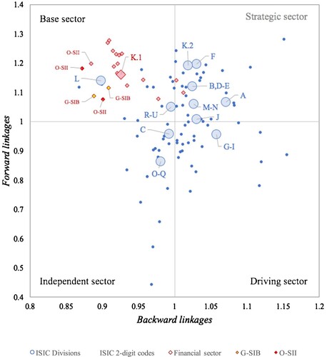
As expected, the financial sector at ISIC results in general terms a forward-oriented sector (Freytag & Fricke, 2017; Rueda-Cantuche et al., 2012), but some exceptions must be made. Observe that in Figure 1, a set of banks fall in the first quadrant, which would be classified accordingly as strategic within the BFL analysis. The possibility of having this type of classification at the level of each bank can be helpful to identify, in great detail, vulnerabilities of the financial system.

For instance, a bank with very strong forward-oriented linkages implies that this financial institution is linked to many different economic activities, using its financial services. In this case, if this financial institution declares bankruptcy, many sectors in the economy will be affected. Comparatively, a bank with weak forward-oriented linkages, concentrating its financial services in just one or few sectors, may generate vulnerabilities if there are negatives economic impacts on the sector on which it depends upon. Linkages among financial institutions and the rest of an economy are relevant concerns for the policy maker during financial crises, mainly because of the risk of financial contagion −a risk that a slight shock to one sector (monetary or not) will propagate to other sectors in a domino effect.

Hypothetical extraction linkage analysis

Table 4 summarizes the main results after applying the HEM on a selection of six banks, those two considered as Global Systemically Important Banks (G-SIB) and the others as Other Systemically Important Institutions (O-SII), this according to the designation established by the BCBS (2018). From these figures, we can see the impact of a bank failure, as a percentage of the loss of value-added, due to hypothetical partial extraction of the financial sector, assuming the bank's specific bankruptcy on the rest of the financial institutions and of the non-financial sectors.

TABLE 4. Percentage value added losses for all sectors due to partial hypothetical extraction of financial sectors (selected systemically important institutions).

		Global systemically important Banks (G-SIB's)		Other systemically important institutions (O-SII's)
Industry (ISIC-Division)		Bank-1	Bank-2	Bank-3	Bank-4	Bank-5	Bank-6
A	Agriculture, forestry and fishing	0.599	0.572	0.422	0.203	0.183	0.101
B,D-E	Mining	0.663	0.639	0.464	0.229	0.201	0.111
C	Manufacturing	0.612	0.580	0.415	0.205	0.184	0.104
F	Construction	1.171	1.063	0.749	0.361	0.348	0.207
G-I	Wholesale and retail trade	0.597	0.577	0.417	0.207	0.181	0.099
J	Information and communication	0.910	0.865	0.550	0.301	0.256	0.154
K.2	Insurance activities	1.014	1.007	0.666	0.365	0.291	0.164
L	Real estate activities	1.023	1.010	0.706	0.367	0.304	0.167
M-N	Professional and business services	0.946	0.916	0.543	0.323	0.255	0.157
O-Q	Public administration and defence	0.210	0.206	0.156	0.075	0.066	0.035
R-U	Other services	0.814	0.799	0.593	0.291	0.251	0.134
K.1	Financial activities	19.972	20.294	14.178	7.254	6.579	3.420
Total Value Added	Median (% loss)	1.160	1.097	0.834	0.389	0.362	0.198
	Standard deviation	0.017	0.019	0.019	0.011	0.007	0.002
	Shapiro-Wilk test (p-value)	0.092	0.423	0.419	0.581	0.858	0.176

Note: From the Shapiro-Wilk normality test, the p-value > 0.05 implying that the distribution of the data are not significantly different from normal distribution. In other words, we can assume the normality.

The lessons learned from the Global Financial Crisis (GFC) were to account for the different sources of systemic risk and the need to monitor each financial institution and the strong linkages between financial institutions and non-financial corporations. In particular, financial stability and banking supervision assess the failure implications of a bank (or group of banks) on the stability of the entire banking system, as well as the channels of risk transmission of macro-financial shocks (IMF-FSB, 2019).

In this way, the hypothetical extraction linkage analysis is useful to understand better the contagion effect under the assumption of bank failures. Hence, the HEM implemented here considers the partial approach as proposed by Dietzenbacher and Lahr (2013) and broadens the scope of this type of analysis by incorporating bankruptcy analysis, which is of broad interest to bank supervision.

However, as pointed out in several studies (Dietzenbacher, 2006; Jansen, 1994; Rueda-Cantuche et al., 2013; Temursho, 2017; ten Raa & Rueda-Cantuche, 2007), we need to pay particular attention to uncertainty issues since it is widely recognized that multiplier estimates within an interindustry context may be biased when the input coefficients assume a random disturbance term as in Equation 6.

Therefore, it is reasonable to note that if fixed-price multiplier matrix is stochastic, the hypothetical extraction analysis may also show an uncertainty bias in their estimates. To deal with the bias, we have carried out a sensitivity analysis based on a Monte Carlo simulations experiment, generating 1,000 datasets following the guidelines of Dietzenbacher (2006) and based on the structure of the error term (see appendix 1).

In order to determine the significance of each hypothetical extraction (bank bankruptcy), a one-sample t-test was conducted to compare the bank’s impact in value-added (% loss). The descriptive statistics (mean value and standard deviation) and normality test results are reported at the bottom of Table 4. Figure 2 presents the distribution for the simulated means, skewness and kurtosis of impact in value added (% loss) for each bank. Similarly, an independent samples t-test corrected for unequal variations (Welch, 1947) was performed to compare the differences between two groups of scores, specifically for between-banks affect upon value added (% loss).²¹

FIGURE 2. Percentage value added losses for all sectors due to partial hypothetical extraction of financial sectors.

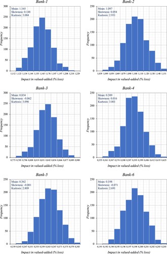
The total impact in valued-added (% loss) goes from the highest impact of 1.16% from Bank-1 (mean expected value with standard deviation equal to 0.016) to the lowest impact of 0.198% from Bank-6 (standard deviation equal to 0.002) for all the economy, being the Construction sector the one that presents the greatest drop in its value-added due to the hypothetical bankruptcy of Bank-1. Due to the relevance of this sector, and the size of the banks, these results are as expected. However, the implication of applying the HEM does not lie only in estimating the possible size of the shock. It rather allows knowing how a financial institution’s deterioration may increase the likelihood of decay of other financial institutions, primarily due to their interlinkages with the non-financial sector in which each financial corporations operate. For example, it is clear that the loss of added value is among the highest in the construction and followed by real estate sectors. By analyzing the detail of the impacts, however, we can observe some heterogeneity in the rest of the results, highlighting, for example, the relative effect of Bank-4 on the real estate activities and insurance activities.

Finally, using Welch’s unequal variances t-test, we find that the difference between bank’s expected values of a bank failure, due to hypothetical partial extraction of a bank, are statistically significant, revealing that under different simulated scenarios have a significant discriminating effect on financial distress.²² The overall picture emerges if we jointly analyze the different scenarios after applying the HEM on a selection of six banks: The greatest mean difference is between G-SIB (Bank-1 and Bank-2) and the O-SII (Bank-3 to Bank-6), and the fewest mean-difference in impact is between the G-SIB and between Bank-4 and Bank-5.

It is worth noting that the bank size should not be considered as the only source of systemic risk. The IMF-FSB (2019) pointed out other determinants that should be considered on this matter (i.e. entity's interconnectivity with other market participants and complexity of its operations and market presence). Hence, using HEM becomes an additional tool to reduce the information gap that bank supervisors have, both the likelihood of bank failure of financial institutions as well as the severity of the effects of any such bankruptcy. Welch’s unequal variances t-test

Structural path analysis

Figures 3 to Figure 5 presents the impulse response functions obtained from the SPA estimates. Under SPA, endogenous accounts multipliers can be considered a pole, which captures the response of an influence (often called a shock) traveling from pole $i$ (origin) to pole $j$ (destination). In this framework, the resulting impulse response analysis provides counterfactual experiments for tracing the marginal effect of a shock to the financial sector (destination) from the real sector (origin) through the path multiplier as expressed in Equation 17.

FIGURE 3. Structural Path Analysis from industry (isic-division) and the effects on selected systemically important institutions.

Source: Own elaboration.

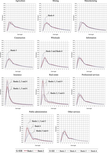
Furthermore, given one standard deviation variation (shock) in gross output by industry (in absolute terms, also referred to as the global totals), the IRF reflects the evolution of the specific response of gross output, along a specified time path, in the selected systemic banks (G-SIB and O-SII). Unraveling the global effects from all paths, elementary path and feedback loop involved, contributes to the idea that contagion in the financial sector is not only a problem of direct linkages. They are part of a complex network made up of the financial and the real sectors.

Figure 3 provides measurements of the response at both levels, macro and micro-level. The origin of the shock refers to the industry at ISIC-Division (macro-aggregate), while the response of the financial sector is presented through the responses observed by systemic institutions (micro-level). As a result, we can highlight four different mechanisms of how contagion risk can spread over the financial system.

The first mechanism is a homogeneous effect. We can notice a similar dynamic of the impulse response function in sectors such as Agriculture, Manufacturing, Information and Professional Services, where the initial response increases between the second path and third path and starts falling afterwards.

The second mechanism occurs in sectors such as construction or commerce. In the first sector, the response of Bank-3 regarding the rest of the institutions in the construction sector stands out, including the sensitivity of Bank-3 and Bank-4 to turbulences originated in the Wholesale sector. These two banks initially react more intensely than the rest of the banks, so we can refer to these two banks as key institutions when analysing the contagion effect from these two specific sectors.

The third mechanism of contagion is observed in the Insurance and Real estate sectors, where the effect shows a cluster response. For instnance, although all banks respond considerably in the first path in the Real estate sector, a group of banks (Bank-1, Bank-3, and Bank-4) responds with more intensity than others. A similar phenomenon occurs in the insurance sector with a similar group of financial firms.

Finally, when analyzing the Public administration sector, we can notice a cascade reaction effect. Under the same original shock, the financial system's reaction takes place in different stages, i.e. the G-SIB and the Bank-5 respond significantly at the second path, followed by the response of Bank-6 at the third path. At the same time, the rest of the banks do it in the fourth path.

All these different effects (homogeneous, key, cluster, and cascade) of a shock reaffirm what was said previously that we should not only take into account the size of banks as the only source of systemic risk. As Harutyunyan and Sánchez (2019) have stressed, policymakers need to detect balance sheet risks and vulnerabilities early enough to be proficient at applying timely responses in terms of economic policy.

The presence of non-financial and financial sectors feedback effects may also give rise to macroeconomic fluctuations during the transitional path, clearly showing that such real and financial links are an important driver of the short-run macroeconomic performance (Bucci et al., 2019). Thus, it is also interesting to provide measurements on how the financial system affects the real side of the economy (which might feed back on the financial system as well).

The fact that interbank network linkages are decisive to understanding the financial fragility of a country's banking system has been known for a long time, but how real sector economy and financial activities affect each other is still an open question (see for example Bucci et al., 2019; and Duffy et al., 2019). In this sense, Figure 4 shows the financial contagion effects, based on a shock where the origin refers to the financial sector (micro-level), while the response of the non-financial sector is observed through the responses observed by industries at ISIC-Division (macro-aggregate).

FIGURE 4. Structural Path Analysis from selected systemically important institutions and the effects on industry (isic-division).

Source: Own elaboration.

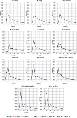
As indicated above, the BFL analysis reveals that the financial sector results in a forward-oriented sector (exhibiting significant forward linkages to the other sectors of the economy), which is likewise spread throughout the rest of the non-financial sectors. As can be seen in Figure 4, there is considerable homogeneity in the impulse response estimates across sector and a strong similarity in the financial contagion effect. Still, we can highlight that while a shock may have a long-lasting effect in sectors like Agriculture, Mining, Manufacturing, or Construction, a similar shock have a sharp-edged response in sectors like real estate, insurance, or public administration.

Therefore, the SPA shed some light on how the interconnectivity between banks with the rest of the sectors can characterize the extent to which financial contagion arising from the financial system propagates to and is determined by the real economy. The methodological framework here proposed become opportune to know how the financial institution interlinkages can provide early warnings on shock propagations among sectors, enabling policymakers to take timely preventive actions and decisions.

Finally, using the SPA decomposition of Section 3.3, we can go deeper into the contagion analysis since it is possible to unravel the transmission channels, showing relevant information about vulnerabilities that are caused directly by the production account (input-output loop) to those caused in intermediate orders (income loop) or those in higher orders accounted by the capital and financial accounts (financial loop).

For example, if we look at the contagion response in the cluster effect formed by Bank-1, Bank-3, and Bank-4 given a shock in Real State sector (see Figure 3), when decomposing the SPA impulse-response, we can identify that behind the early response of this group of banks is acting the high interconnectedness with the productive system (input-output loop). Bank-1 in the third path accumulates 47% of the total impact effect, Bank-3 accumulates 42%, and Bank-4 accumulates 51% of the total impact (mainly intermediate consumption and value-added interlinkages). At the same time, the rest of the banks mainly responded for their interrelations with the income loop (accounted by the distribution and use of income accounts interlinkages) and distributed over different paths (Table 5).

TABLE 5. Structural path analysis decomposition selected sector: real state.

	Shock from: Real estate activities
	Bank-1			Bank-2			Bank-3			Bank-4			Bank-5			Bank-6
Path lenght	IO	SAM	FSAM	IO	SAM	FSAM	IO	SAM	FSAM	IO	SAM	FSAM	IO	SAM	FSAM	IO	SAM	FSAM
1	–	–	–	–	–	–	–	–	–	–	–	–	–	–	–	–	–	–
2	43.54	–	–	19.15	–	–	36.24	–	–	46.38	–	–	18.07	–	–	13.16	–	–
3	3.10	7.27	–	7.93	8.06	–	5.71	4.13	–	4.85	2.84	–	4.69	10.16	–	3.46	14.34	–
4	0.96	6.06	–	2.06	7.23	–	1.51	5.84	–	1.39	5.40	–	1.54	8.22	–	1.13	9.18	–
5	0.34	3.95	0.00	0.72	5.97	–	0.57	5.72	0.01	0.53	4.78	0.01	0.57	5.87	0.00	0.41	5.31	0.00
6	0.13	4.11	0.13	0.28	5.72	0.01	0.22	4.16	0.30	0.21	3.47	0.19	0.22	6.07	0.20	0.16	6.76	0.14
7	0.06	3.65	0.27	0.11	4.85	0.21	0.09	3.79	0.45	0.09	3.34	0.31	0.09	5.22	0.40	0.06	5.64	0.37
8	0.02	2.77	0.38	0.05	3.81	0.42	0.04	3.03	0.57	0.04	2.68	0.42	0.04	4.01	0.57	0.03	4.21	0.54
9	0.01	2.20	0.45	0.02	3.02	0.57	0.02	2.34	0.66	0.02	2.06	0.50	0.02	3.19	0.67	0.01	3.41	0.64
10	0.00	1.72	0.51	0.01	2.36	0.67	0.01	1.85	0.72	0.01	1.64	0.55	0.01	2.49	0.75	0.00	2.64	0.73
11	0.00	1.34	0.55	0.00	1.85	0.75	0.00	1.45	0.76	0.00	1.28	0.59	0.00	1.94	0.82	0.00	2.05	0.81
12	0.00	1.06	0.58	0.00	1.46	0.81	0.00	1.14	0.78	0.00	1.00	0.61	0.00	1.53	0.86	0.00	1.63	0.86
13	0.00	0.83	0.60	0.00	1.15	0.85	0.00	0.90	0.79	0.00	0.79	0.62	0.00	1.21	0.89	0.00	1.28	0.88
14	0.00	0.65	0.60	0.00	0.90	0.87	0.00	0.70	0.79	0.00	0.62	0.63	0.00	0.95	0.89	0.00	1.00	0.89
15	0.00	0.51	0.60	0.00	0.71	0.88	0.00	0.55	0.77	0.00	0.49	0.62	0.00	0.74	0.89	0.00	0.79	0.89
Total	48.2	38.0	13.8	30.3	49.7	20.0	44.4	37.6	18.0	53.5	32.2	14.3	25.2	54.3	20.4	18.4	61.1	20.5

 Besides, we can also know that the propagation reaction is less vulnerable given the feedback effect with the capital and financial intermediation accounts (e.g. Bank-2 reaction due to financial interconnectedness is observed in path six, while Bank-4 in the fourth path shown reaction linked to the financial loop).

As mentioned above; the SPA cannot acknowledge all the structural and behavioral mechanisms that result in the accounting multipliers. Thus, to understand the intricated links between macroeconomic conditions and the systemic risks embedded in the financial systems, the SPA decomposition becomes relevant to unveil the network of financial and real paths along with a shock that travels through the economy. Understanding risk determinants and channels of risk transmission of macro-financial shocks between economics agents result in an outstanding analytical tool in the fields of macroeconomic and financial stability analysis.

5. Conclusions and scope for future research

The social accounting matrix (SAM) system provides the best available framework for reconciling the accounts of micro actors with the macroeconomic aggregates, which have traditionally been the focus of statistical data. However, it is still latent that micro- and macro-prudential analysis need macrodata and granular microdata to identify, measure, and monitor better the financial risk in an economy. Our main contribution relies on developing an applied framework for policymakers and analysts of macro-micro financial linkages within an input-output (IO) economy. Dealing with the appropriate methodological approaches, the results presented in this research show how it is feasible to include individual bank information into the financial SAM (FSAM) framework, keeping the inherent accounting rules and ensuring that the balances are satisfied.

The proposed framework allows understanding and appraising the mechanisms by which shocks to the financial sector can result in a feedback loop to the real sectors; in other words, contagion effects within the financial sector. Extending the macro-financial linkages analysis through an accounting multiplier setting provides a powerful tool for systemic risk analysis, showing how the wealth of the information supplied by financial accounts embedded in an FSAM framework can support public policy. Also, it provides a consistent accounting framework that allows a detailed analysis of the financial sector and the structure of an economy as a whole.

This novel research provides noteworthy methodological contributions, which align with the usage of existing datasets to build FSAMs and its fixed-price multiplier model with the implementation HEM and SPA, to understand financial linkages and their role in systemic risk. Henceforth, analysts and policymakers can further evaluate financial stability, external vulnerability, fiscal sustainability, and domestic and global interconnectedness while contributing to the existing discussions and knowledge required by IMF-FSB (2018).

The methodological and empirical results presented in the research increase data coverage and fundamental analysis of both financial and non-financial sectors. Furthermore, the methodology allows covering the requirements made by the DGI-2 to go further on developing new mechanisms of integration of macro/micro-information and upgrading the financial stability models and frameworks (Lima & Drumond, 2016).

The results contribute directly to the recommendation II.8 on sectorial accounts, dealing with one of the main challenges regarding granular and consistent data of institutional sectors and from-whom-to-whom information to understand better the intersectoral linkages. Furthermore, the finding also extends the analysis of the financial soundness indicators (FSI), since it manages concentration and distribution measures (CDM) of Global Systemically Important Banks (G-SIBs). In sum, this paper suggests that an FSAM framework that embeds micro-macro linkages enhances the actual use of financial accounts information and may be considered an additional angle of attack on some open issues in macro-financial crises analysis.

At the present time, the main source of macroeconomic instability is the devastating effect that coronavirus pandemic (COVID-19) is leaving on the economy, health and the financial system. The sudden outbreak of COVID-19 has made firms globally face extreme financial limitations, and this period of crises is characterized by a shock that does not emanate from the financial sector or from a particular firm or industry. In this times, the instability arise from an exogenous health shock, in which almost all aspects of the current crisis have been surrounded by significant uncertainty regarding its magnitude and duration on economic activity worldwide.

Although specific policy analysis is beyond the scope of this research, we believe that the theoretical framework could be adapted to review, from a renewed general equilibrium perspective, the analysis of public-policy support to firms under financial constraints. Therefore, a future study can be done to identify the the magnitude of the pandemic crisis, the speed of the eventual recovery, and the effectiveness of different policies.

The links between activities are likely to play a relevant role in transmitting the economic shock resulting from COVID-19 containment policies (Demirgüç-Kunt et al., 2020). Since the banking sector plays a fundamental intermediary role in channeling funding sources to productive activities, failure in this function could significantly aggravate the already sizable economic impact of the current pandemic shock (Beck, 2020). Policymakers must be insightful until the health crisis is resolved, adopting policies oriented to reduce the shock and the impact of the containment measures on the real sector (Didier et al., 2021). The approach proposed by this research can be used to answer some misunderstood effects of different policy interventions to sustain firm financing without losing focus on financial stability.

Disclosure statement

No potential conflict of interest was reported by the author(s).

Notes

1 Bremus et al. (2018) points out that among the small number of recent empirical works studying risk interactions effects of heterogeneous banks for macroeconomic outcomes are the works of Blank et al. (2009), Buch and Neugebauer (2011) and Carvalho and Gabaix (2013).

2 The IAG members are BIS, ECB, Eurostat, IMF (chair), OECD, United Nations and World Bank.

3 In particular, we have devoted special attention to the DGI-2 recommendations; for instance: II.2 Concentration and distribution measures related to Financial Soundness Indicators; II.3 Recongnition of Global Systemically Important Institutions; II.4 Household distributional information and understanding of intersectoral linkages; II.8 Granular and consistent institutional sector accounts data and from-whom-to-whom information, and information transparency; and finally II.9 Development and dissemination of distributional information on income, consumption, saving and wealth for the household sector.

4 The endogenous accounts are the ones considered into the accounting multiplier used in this paper. In addition, the complete FSAM also consider the government account and the rest of the world accounts as exogenous accounts.

5 Each account consists of a set of submatrices defined by the symmetric dimension of commodities and industries ($m$), value-added categories ($k$), institutional sector ($p$), non financial assets ($g$), and/or financial instruments ($q$).

6 In order to simplify the explanation, the sub matrices relative to the secondary distribution of income allocation and taxes less subsidies are not explicit in this scheme. However, they have been incorporated into the ${\mathbf{T}}_{\text{FSAM}}$.

7 Throughout this work, matrices are indicated by bold, capital letters; vectors by bold, lower-case letters; and scalars by italicized lower-case letters. By definition vectors are strictly columns, so that row vectors are denoted by transposition (a prime symbol '). Finally a diagonal matrix with the elements of any vector on its main diagonal and all other entries equal to zero are indicated by a circumflex.

8 According to United Nations et al. (2008), when considering the financial sector alone or in connection with other statistics such as monetary and financial statistics, it is usual to speak of financial institutions rather than financial corporations. Given that no change in definition or coverage is implied by this change in terminology we will use both terminologies indistinguishably.

9 Past studies of market concentration in Europe have instead used the regional distribution of branch offices (which is known) to compute a Herfindahl-Hirschman index of market concentration and sectoral credit risk by industry.

10 Specifically, it refers to the activity ‘64 Financial service activities, except insurance and pension funding' according to ISIC (Revision 4).

11 In accordance with the Basel III framework, implemented in Europe through Directive 2013/36 and Regulation 575/2013 on prudential requirements for credit institutions and investment firms, the financial sector is required to present a disclosure report on the Pillar 3 with the disclosure and market information requirements covering credit exposure by industry.

12 See Temurshoev (2015) for a recent survey of uncertainty treatment in input-output analysis.

13 The alternative inverse model formulation of the inter-industry model suggested by Ghosh (1958) is based in its direct sales coefficients matrix, $\tilde{\mathbf{A}}={\hat{\mathbf{y}}}^{-1}\mathbf{T}$. As have been shown by Lenzen (2003), the fundamental equation of this model links exogenous primary inputs $\mathbf{v}$ with total output such that ${\mathbf{y}}^{\mathrm{\prime }}=\mathbf{v}(\mathbf{I}-\tilde{\mathbf{A}}{)}^{-1}=\mathbf{v}\tilde{M}$.

14 See Miller and Blair (2009) and Dietzenbacher and Lahr (2013) for morinsight and other extensions.

15 The results can be then referred to a single sector by assuming $m_1$ = 1

16 We consider the case in which the final demand remain the same, corresponding the case where one bank $n$. in the financial sector has ceased to exist and, therefore, the financial services of this sector decrease. The financial institution’s final demands, however, are somehow met by the remaining financial institutions in this sector.

17 Aldasoro and Angeloni (2014) is focused in a linkages analysis (backward and forward) to measure the systemic importance of financial institutions.

18 In economics, and especially in contemporary macroeconomic modeling, impulse response functions are used to describe how the economy reacts over time to exogenous impulses, which economists

usually call shocks, and are often modeled in the context of a vector autoregression models and DSGE models (Lütkepohl, 2008).

19 An important feature to be considered is that the SNA uses various information classifiers contained in the INE and BdE statistics. These information classifiers were maintained and used to present the dataset.

20 In accordance with the Basel III framework, implemented in Europe through Directive 2013/36 and Regulation 575/2013 on prudential requirements for credit institutions and investment firms, the financial sector is required to present a disclosure report on the Pillar III with the disclosure and market information requirements covering credit exposure by industry.

21 The independent samples t-test corrected for unequal variances is commonly known as Welch’s test, and is widely considered to be more robust than Student's t-test and maintains type I error rates close to nominal for unequal variances and for unequal sample sizes under normality.

22 The mean-difference in value added were calculated and there was no significant differences among all possible combinations. After Welch’s unequal variances t-test all p-value < 0.01, thefore true difference in means were not equal to 0.

References

- Achjar, N., Sonis, M., & Hewings, G. J. D. (2006). Structural changes in the Indonesian economy: A network complication approach. Journal of Applied Input–Output Analysis, 11, 91–119.
- Aldasoro, I., & Angeloni, I. (2015). Input–output-based measures of systemic importance. Quantitative Finance, 15(4), 589–606. doi:10.1080/14697688.2014.968194
- Amiti, M., & Weinstein, D. E. (2018). How much do idiosyncratic bank shocks affect investment? Evidence from matched bank-firm loan data. Journal of Political Economy, 126(2), 525–587. doi:10.1086/696272
- Aray, H., Pedauga, L., & Velázquez, A. (2017). Financial Social Accounting Matrix: a useful tool for understanding the macro-financial linkages of an economy. Economic Systems Research, 29(4), 486–508. doi:10.1080/09535314.2017.1365049
- Banco de España. (2019). Cuentas Financieras de la Economía Española. www.bde.es (observed 5 May 2020).
- Basel Committee on Banking Supervision. (2011). Global systemically important banks: Assessment methodology and the additional loss absorbency requirement, Bank for International Settlements, Basel, November.
- Basel Committee on Banking Supervision. (2017a). Standards: Pillar 3 disclosure: requirements – consolidated and enhanced framework. Bank for International Settlements, Basel, March.
- Basel Committee on Banking Supervision. (2017b). Global systemically important banks - revised assessment framework, Consultative document, Bank for International Settlements, Basel, March.
- Basel Committee on Banking Supervision. (2018). Global systemically important banks: revised assessment methodology and the higher loss absorbency requirement, Bank of International Settlements, Basel, July.
- Beck, T. (2020). Finance in times of COVID-19: What next. Mitigating the Covid Economic Crisis: Act Fast and Do Whatever It Takes, edited by R. Baldwin and BW di Mauro, VOXEu. org Book.
- Bezemer, D. J. (2010). Understanding financial crisis through accounting models. Accounting, Organizations and Society, 35(7), 676–668. doi:10.1016/j.aos.2010.07.002
- Blank, S., Buch, C. M., & Neugebauer, K. (2009). Shocks at large banks and banking sector distress: The Banking granular residual. Journal of Financial Stability, 5(4), 353–373. doi:10.1016/j.jfs.2008.12.002
- Borio, C. (2013). The great financial crisis: Setting priorities for new statistics. Journal of Banking Regulation, 14(3–4), 306–317. doi:10.1057/jbr.2013.9
- Bremus, F., & Buch, C. M. (2017). Granularity in banking and growth: Does financial openness matter? Journal of Banking & Finance, 77, 300–316. doi:10.1016/j.jbankfin.2016.04.023
- Bremus, F., Buch, C. M., Russ, K. N., & Schnitzer, M. (2018). Big banks and macroeconomic outcomes: Theory and cross-country evidence of granularity. Journal of Money, Credit and Banking, 50(8), 1785–1825. doi:10.1111/jmcb.12545
- Bucci, A., La Torre, D., Liuzzi, D., & Marsiglio, S. (2019). Financial contagion and economic development: An epidemiological approach. Journal of Economic Behavior & Organization, 162, 211–228. doi:10.1016/j.jebo.2018.12.018
- Buch, C. M., & Neugebauer, K. (2011). Bank-specific shocks and the real economy. Journal of Banking & Finance, 35(8), 2179–2187. doi:10.1016/j.jbankfin.2011.01.023
- Burgess, S. (2011). Measuring financial sector output and its contribution to UK GDP. Bank of England Quarterly Bulletin, 51(3), 234–246.
- Cai, J., & Leung, P. (2004). Linkage measures: A revisit and a suggested alternative. Technology Analysis & Strategic Management, 16(1), 63–83. doi:10.1080/0953531032000164800a
- Carbó-Valverde, S., Humphrey, D., & Rodríguez, F. (2003). Deregulation, bank competition and regional growth. Regional Studies, 37(3), 227–237. doi:10.1080/0034340032000065398
- Carbó-Valverde, S., & Rodríguez, F. (2004). The finance-growth nexus: A regional perspective. European Urban and Regional Studies, 11(4), 339–354. doi:10.1177/0969776404046265
- Cardenete, M., Lima, M., & Sancho, F. (2013). Are there key sectors? An appraisal using applied general equilibrium. Review of Regional Studies, 43(2, 3), 111–129. https:/doi.org/10.52324/001c.8087
- Cardenete, M., & Sancho, F. (2006). Missing links in key sector analysis. Economic Systems Research, 18(3), 319–325. doi:10.1080/09535310600844409
- Clements, B. J. (1990). On the decomposition and normalization of interindustry linkages. Economics Letters, 33(4), 337–340. doi:10.1016/0165-1765(90)90084-E
- Defourny, J., & Thorbecke, E. (1984). Structural path analysis and multiplier decomposition within a social accounting matrix framework. The Economic Journal, 94(373), 111–136. doi:10.2307/2232220
- Demirgüç-Kunt, A., & Levine, R. (2018). Finance and growth. Edward Elgar Publishing Limited.
- Demirgüç-Kunt, A., Pedraza, A., & Ruiz Ortega, C. (2020). Banking sector performance during the covid-19 crisis. World Bank Policy Research Working Paper, 9363.
- Didier, T., Huneeus, F., Larrain, M., & Schmukler, S. L. (2021). Financing firms in hibernation during the COVID-19 pandemic. Journal of Financial Stability, 53, 100837. doi:10.1016/j.jfs.2020.100837
- Dietzenbacher, E. (2006). Multiplier estimates: To bias or not to bias? Journal of Regional Science, 46(4), 773–786. doi:10.1111/j.1467-9787.2006.00477.x
- Dietzenbacher, E., & Lahr, M. L. (2013). Expanding extractions. Economic Systems Research, 25(3), 341–360. doi:10.1080/09535314.2013.774266
- Dietzenbacher, E., van Burken, B., & Kondo, Y. (2019). Hypothetical extractions from a global perspective. Economic Systems Research, 31(4), 505–519. https://doi.org/10.1080/09535314.2018.1564135
- Dietzenbacher, E., & Van der Linden, J. A. (1997). Sectoral and spatial linkages in the EC production structure. Journal of Regional Science, 37(2), 235–257. doi:10.1111/0022-4146.00053
- Duffy, J., Karadimitropoulou, A., & Parravano, M. (2019). Financial contagion in the laboratory: Does network structure matter? Journal of Money, Credit and Banking, 51(5), 1097–1136. doi:10.1111/jmcb.12563
- Emini, C. A., & Fofack, H. (2004). A financial social accounting matrix for the integrated macroeconomic model for poverty analysis: Application to Cameroon with a fixed-price multiplier analysis. Vol. 3219. World Bank Publications.
- Evans, O., Leone, A. M., Gill, M., & Hilbers, P. (2000). Macroprudential Indicators of Financial System Soundness, IMF Occasional Paper, 192.
- Fernandez de Guevara, J., & Maudos, J. (2007). Regional financial development and bank competition: effects on economic growth, MPRA Paper 15255, University Library of Munich, Germany.
- Financial Stability Board. (2018). Global Shadow Banking Monitoring Report 2017. Financial Stability Board: Basel.
- Freytag, A., & Fricke, S. (2017). Sectoral linkages of financial services as channels of economic development – An input–output analysis of the Nigerian and Kenyan economies. Review of Development Finance, 7(1), 36–44. doi:10.1016/j.rdf.2017.01.004
- Gabaix, X. (2011). The granular origins of aggregate fluctuations. Econometrica, 79(3), 733–772. doi:10.3982/ECTA8769
- Guerra, A. I., & Sancho, F. (2010). Measuring energy linkages with the hypothetical extraction method: An application to Spain. Energy Economics, 32(4), 831–837. doi:10.1016/j.eneco.2009.10.017
- Hanson, K. A., & Robinson, S. (1991). Data, linkages and models: US national income and product accounts in the framework of a social accounting matrix. Economic Systems Research, 3(3), 215–232. doi:10.1080/09535319100000019
- Harutyunyan, A., & Sánchez, C. (2019). The IMF balance sheet approach: Towards from-whom-to-whom information on cross-border portfolio securities. IFC Bulletins Chapters, 49, 300–317.
- Hazari, B. R. (1970). Empirical identification of key sectors in the Indian economy. The Review of Economics and Statistics, 52(3), 301–305. doi:10.2307/1926298
- Heath, R., & Goksu, E. (2016). G-20 Data gaps initiative II: Meeting the policy challenge, IMF Working Paper, WP/16/43.
- Heath, R., & Goksu, E. (2017). Financial stability analysis: What are the data needs? IMF Working Paper 17/153, International Monetary Fund, Washington, DC.
- Hirschman, Albert (1958). The strategy of economic development. New Haven, Conn.: Yale Univ. Press.
- Hubic, A. (2012). A Financial Social Accounting Matrix (SAM) for Luxembourg, Working Paper, 2008–72, Central Bank of Luxembourg.
- International Monetary Fund & Financial Stability Board. (2009). The financial crisis and information gaps, Report to the G20 Finance Ministers and Central Bank Governors, October.
- International Monetary Fund & Financial Stability Board. (2015). The Financial Crisis and Information Gaps: Sixth Progress Report on the Implementation of the G-20 Data Gaps Initiative, technical report, September, http://www.fsb.org/wp-content/uploads/The-Financial-Crisis-and-Information-Gaps.pdf.
- International Monetary Fund & Financial Stability Board. (2018). Implementation and Effects of the G20 Financial Regulatory Reforms: 5th Annual Report. Basel.
- International Monetary Fund & Financial Stability Board. (2019). G20 Data Gaps Initiative (DGI-2): The Fourth Progress Report - Countdown to 2021. Basel.
- Jamshidian, M., & Mata, M. (2007). Advances in analysis of mean and covariance structure when data are incomplete. In Handbook of latent variable and related models (pp. 21–44). North-Holland.
- Jansen, P. (1994). Analysis of multipliers in stochastic input-output models. Regional Science and Urban Economics, 24(1), 55–74. doi:10.1016/0166-0462(94)90019-1
- Kasinger, J., & Pelizzon, L. (2018). Financial stability in the EU: A case for micro data transparency. SAFE Policy Letter, 67, 1–9.
- Lenzen, M. (2003). Environmentally important paths, linkages and key sectors in the Australian economy. Structural Change and Economic Dynamics, 14(1), 1–34. doi:10.1016/S0954-349X(02)00025-5
- Lenzen, M. (2007). Structural path analysis of ecosystem networks. Ecological Modelling, 200(3–4), 334–342. doi:10.1016/j.ecolmodel.2006.07.041
- Lima, F., & Drumond, I. (2016). How to keep statistics’ customers happy? Use micro-databases!. IFC Bulletin No 41. Bank of International Settlements.
- Luo, J. (2013). Which industries to bail out first in economic recession? Ranking US industrial sectors by the power-of-pull. Economic Systems Research, 25(2), 157–169. doi:10.1080/09535314.2013.775111
- Lütkepohl, H. (2008). Impulse response function. In P. Macmillan (Ed.), The New Palgrave dictionary of economics. Palgrave Macmillan. https://doi.org/10.1057/978-1-349-95121-5_2410-1
- Miller, R. E. (1966). Interregional feedback effects in input-output models: Some preliminary results. Papers of the Regional Science Association, 17(1), 105–125. doi:10.1007/BF01982512
- Miller, R. E., & Blair, P. D. (2009). Input-output analysis: Foundations and extensions. Cambridge University Press.
- Miller, R. E., & Lahr, M. L. (2001). A taxonomy of extractions. In M. L. Lahr & R. E. Miller (Eds.), Regional science perspectives in economic analysis – a festschrift in memory of Benjamin H. Stevens (pp. 407–441). North-Holland.
- Paelinck, J., De Caevel, J., & Degueldre, J. (1965). Analyse quantitative de certaines phénomenes du développment régional polarisé: Essai de simulation statique d’itérarires de propogation. Bibliothèque de L’Institut de Science économique, 7, 341–387.
- Pedauga, L., Velázquez, A., & Bueno, M. (2018). Property income from-whom-to-whom matrices: A dataset based on financial assets–liabilities stocks of financial instrument for Spain. Data in Brief, 19, 449–455. doi:10.1016/j.dib.2018.05.018
- Perobelli, F. S., Faria, W. R., & de Almeida Vale, V. (2015). The increase in Brazilian household income and its impact on CO2 emissions: Evidence for 2003 and 2009 from input–output tables. Energy Economics, 52, 228–239. doi:10.1016/j.eneco.2015.10.007
- Pyatt, G. (1988). A SAM approach to modeling. Journal of Policy Modeling, 10(3), 327–352. doi:10.1016/0161-8938(88)90026-9
- Rasmussen, N. P. (1956). Studies in intersectoral relations. North Holland Publishing Co.
- Roland-Holst, D. W., & Sancho, F. (1995). Modeling prices in a SAM structure. The Review of Economics and Statistics, 77(2), 361–371. doi:10.2307/2109871
- Rueda-Cantuche, J. M., Dietzenbacher, E., Fernández, E., & Amores, A. F. (2013). The bias of the multiplier matrix when supply and use tables are stochastic. Economic Systems Research, 25(4), 435–448. doi:10.1080/09535314.2013.776947
- Rueda-Cantuche, J. M., Kratena, K., Streicher, G., Neuwahl, F., Mongelli, I., Rueda-Cantuche, J. M., Genty, A., Arto, I., & Andreoni, V. (2012). FIDELIO: A Fully Interregional Dynamic Econometric Long-Term Input-Output Model for the EU, EcoMod2012, N° 4082, EcoMod.
- Saldías, M. (2011). Sectoral credit risk in the euro area. Economic Bulletin and Financial Stability Report Articles and Banco de Portugal Economic Studies.
- Stock, J. H., & Watson, M. W. (2001). Vector autoregressions. The Journal of Economic Perspectives, 15(4), 101–115. doi:10.1257/jep.15.4.101
- Strassert, G. (1968). Zur bestimmung strategischer sektoren mit hilfe von input-output-modellen. Jahrbücher für Nationalökonomie und Statistik, 182(1), 211–215. doi:10.1515/jbnst-1968-0114
- Temursho, U. (2017). Uncertainty treatment in input–output analysis. In Handbook of Input–Output Analysis. Edward Elgar Publishing.
- Temurshoev, U. (2010). Identifying optimal sector groupings with the hypothetical extraction method. Journal of Regional Science, 50(4), 872–890. doi:10.1111/j.1467-9787.2010.00678.x
- ten Raa, T. T., & Rueda-Cantuche, J. M. (2007). Stochastic analysis of input–output multipliers on the basis of use and make tables. Review of Income and Wealth, 53(2), 318–334. doi:10.1111/j.1475-4991.2007.00227.x
- Thorbecke, E. (2000). The use of social accounting matrices in modeling. Paper presented at the 26th General conference of the international association for research in income and wealth, Krakow, Poland, August 27–September 2, 2000.
- Tissot, B. (2016). Closing information gaps at the global level – what micro data can bring, IFC Bulletin, no 41, May.
- Tsujimura, K., & Tsujimura, M. (2010). A flow-of-funds analysis of quantitative monetary policy. In S. Ichimura, & L. R. Klein (Eds.), Macroeconometric analysis of Japan (pp. 173–193). World Scientific.
- United Nations, Commission of the European Communities, International Monetary Fund, Organization for Economic Co-operation & Development and World Bank. (2008). System of National Accounts 2008. World Bank.
- van de Ven, P., & Fano, D. (2017). Understanding financial accounts. OECD Publishing.
- Welch, B. L. (1947). The generalization of student’s problem when several different population variances are involved. Biometrika, 34(1–2), 28–35. https://doi.org/10.1093/biomet/34.1-2.28
- Wood, R., & Lenzen, M. (2009). Structural path decomposition. Energy Economics, 31(3), 335–341. doi:10.1016/j.eneco.2008.11.003
- Zhao, Y., Wang, S., Liu, Y., Zhang, Z., Zhang, Y., & Li, H. (2017). Identifying the economic and environmental impacts of China's trade in intermediates within the Asia-pacific region. Journal of Cleaner Production, 149, 164–179. doi:10.1016/j.jclepro.2017.02.085