Price re-interpretations of the basic IO quantity models result in the ultimate input-output equations

Abstract

This note shows that Leontief's well-known demand-driven input–output (IO) quantity model may also be interpreted as the almost unknown revenue-pull IO price model, but measured in value terms instead of in prices. It is also shown how these two demand-driven models may be combined into a single ultimate demand-driven IO equation. An analogous result holds for the supply-driven quantity model and the cost-push price model, which results in a single ultimate supply-driven IO equation. The new price interpretation of the Leontief quantity model opens up hitherto unused possibilities to simulate interindustry demand-driven inflation processes, just as the price interpretation of the Ghosh quantity model enables simulations of supply-driven inflation processes.

KEYWORDS:

• Leontief model
• Ghosh model
• Supply-driven inflation
• Demand-driven inflation
• Ultimate input–output equations

1. Introduction

The four basic input–output (IO) models are mathematically very similar, but economically they are worlds apart. The two quantity models are each other’s mirror image, as are their corresponding, two price models. The demand-driven IO quantity model (Leontief, 1941) and its cost-push IO price dual (Leontief, 1951) are well known. The supply-driven IO quantity model (Ghosh, 1958) is less known and – for good reasons – has hardly been used since the 1990s. Its revenue-pull IO price dual (Davar, 1989; Oosterhaven, 1989) is not known at all and has never been used, despite its potential.

This note shows that this least known IO model can be rewritten such that it mimics the best known IO model, i.e. it mimics Leontief's quantity model, which therefor may also be interpreted as the Davar/Oosterhaven price model measured in value terms instead of in prices. As such, it may empirically be used to simulate demand-driven inflation processes, as opposed to supply-driven inflation processes that may be simulated with Leontief's cost-push price model.

Before proving and explaining this new model interpretation, we briefly summarize the four basic IO models and present a more elegant proof for the re-interpretation of the Ghosh quantity model as the Leontief price model measured in values instead of in prices (Dietzenbacher, 1997). Besides, we show that the solution of both supply-driven models, as well as that of both demand-driven models, can be combined into one single, ultimate IO equation.

2. The four basic input–output models

All four basic IO models are based on the accounting identities of the industry-by-industry type of input–output table (IOT) shown in Table 1, which also contains the definitions of the vectors and matrices used in this note. In Table 1 and elsewhere, the symbol $\in$ is used to indicate that the scalar or equation on its left-hand side represents the typical element or the typical equation of the matrix formulation on its right-hand side, e.g. $y_{\mathrm{iq}}\in \mathbf{\text{Y}}$ in Table 1 indicates that the matrix with final outputs Y has $y_{\mathrm{iq}}$ as its typical element, with i = 1, … , I and q = 1, … , Q, where I = the number of industries and Q = the number of final demand categories. Analogously, $v_{\mathrm{pj}}=c_{\mathrm{pj}}{x}_j\in \mathbf{\text{V}}\mathbf{\text{i}}=\mathbf{\text{C}}\mathbf{\text{x}}$ in the text just above (1) indicates how, in the Leontief model, primary inputs $v_{\mathrm{pj}}\in \mathbf{\text{V}}$ are determined by fixed primary input coefficients $c_{\mathrm{pj}}\in \mathbf{\text{C}}$ and total output $x_j\in \mathbf{\text{x}}$, with p = 1, … , P and j = 1, … , I, where P = number of primary input categories.

Table 1. Input–output table with macro totals.

	Industries	Final demand	Total output
Industries	$z_{\mathrm{ij}}\in \mathbf{\text{Z}}$	$y_{\mathrm{iq}}\in \mathbf{\text{Y}}$	$x_i\in \mathbf{\text{x}}$
Primary supply	$v_{\mathrm{pj}}\in \mathbf{\text{V}}$	$r_{\mathrm{pq}}\in \mathbf{\text{R}}$	M Y
Total input	$x_j\in {\mathbf{\text{x}}}^{\mathrm{\prime }}$	C I G E

IOTs are always expressed in monetary values. For IO modeling purposes, these monetary values are treated as quantities measured in unit prices with the value one, which is how the symbols in Table 1 will be interpreted in this note. Consequently, prices in this note do not represent real prices but index prices that all have a value of one in the base year of the IOT. Table 1, by the way, also shows that an IOT essentially represents a double sectoral breakdown of the well-known macro-economic accounting identity for the Gross Domestic Product: Y = C + I + G + E – M. Italics are used to indicate scalars, whereas bold lower cases indicate vectors and bold capitals indicate matrices. A summation column with ones is indicated by i, while a summation row with ones is indicated by i'.

Both sets of input–output models may be given a microeconomic foundation, as both sets may be based on simplifications of the most general production function with multiple inputs and multiple outputs, as measured in Table 1's columns and rows, respectively. The pair of Leontief models assumes single homogenous outputs across the rows of the IOT, each with a uniform price, along with heterogeneous inputs with different prices across its columns, whereas the Ghosh/Davar pair of models assumes single homogenous inputs across the columns of the IOT, each with a uniform price, along with heterogenous outputs with different prices across its rows (see the Appendix for all assumptions of both sets of models).¹

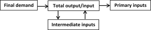
In the classic demand-driven IO quantity model, along the rows of the IOT, total exogenous final demand quantities $\mathbf{\text{y}}=\mathbf{\text{Y}}\mathbf{\text{i}}$, along with total endogenous intermediate demand quantities $\mathbf{\text{Z}}\mathbf{\text{i}}$, determines the size of total output, i.e. $\mathbf{\text{x}}=\mathbf{\text{Z}}\mathbf{\text{i}}+\mathbf{\text{y}}$. At constant prices, total output, in turn, backwardly along the columns of the IOT, determines the use of both intermediate and primary inputs by means of fixed intermediate input coefficients $z_{\mathrm{ij}}=a_{\mathrm{ij}}{x}_j\in \mathbf{\text{Z}}\mathbf{\text{i}}=\mathbf{\text{A}}\mathbf{\text{x}}$ and fixed primary input coefficients $v_{\mathrm{pj}}=c_{\mathrm{pj}}{x}_j\in \mathbf{\text{V}}\mathbf{\text{i}}=\mathbf{\text{C}}\mathbf{\text{x}}$, with ${\mathbf{\text{i}}}^{\mathrm{\prime }}\mathbf{\text{A}}+{\mathbf{\text{i}}}^{\mathrm{\prime }}\mathbf{\text{C}}={\mathbf{\text{i}}}^{\mathrm{\prime }}$. The changes in intermediate inputs subsequently lead to further and further backward effects on total output (see Figure 1). The solutions for total output, intermediate inputs, and primary inputs (i.e. imports and value added) then, respectively, read as follows: (1) $\mathbf{\text{x}}=\mathbf{\text{A}}\mathbf{\text{x}}+\mathbf{\text{y}}\Rightarrow \mathbf{\text{x}}=(\mathbf{\text{I}}-\mathbf{\text{A}}{)}^{-1}\mathbf{\text{y}}=\mathbf{\text{L}}\mathbf{\text{y}},\mathbf{\text{Z}}\mathbf{\text{i}}=\mathbf{\text{A}}\mathbf{\text{L}}\mathbf{\text{y}}\text{and}\mathbf{\text{V}}\mathbf{\text{i}}=\mathbf{\text{C}}\mathbf{\text{L}}\mathbf{\text{y}}$(1) where $\mathbf{\text{L}}$ = the Leontief-inverse. Obviously, reality only comes close to this model when all markets are characterized by excess supply, i.e. around the bottom of the business cycle, but even then price reactions may dampen the predicted quantity changes (see further Oosterhaven, 2022, Ch. 7)

Figure 1. Common causal structure of the demand-driven IO price and quantity model.

The cost-push price dual of this classic IO model, along the columns of Table 1, assumes that exogenous primary input prices $p_p\in {\mathbf{\text{p}}}_v$, along with endogenous intermediate input prices $p_i\in \mathbf{\text{p}}$, weighted with their respective cost shares $\mathbf{\text{C}}$ and $\mathbf{\text{A}}$, determine the cost and price of total inputs $p_j={\sum }_i{p}_i{a}_{\mathrm{ij}}+{\sum }_p{p}_p{c}_{\mathrm{pj}}\in {\mathbf{\text{p}}}^{\mathrm{\prime }}={\mathbf{\text{p}}}^{\mathrm{\prime }}\mathbf{\text{A}}+{{\mathbf{\text{p}}}^{\mathrm{\prime }}}_v\mathbf{\text{C}}$. At constant quantities, any change in the cost of total inputs is passed on uniformly, along the rows of the IOT, to all intermediate and final users of the outputs of the industry at hand. The changes in the prices of intermediate inputs are subsequently passed on further and further (see Figure 2). The solution for the prices of total output/input then reads as follows: (2) ${\mathbf{\text{p}}}^{\mathrm{\prime }}={\mathbf{\text{p}}}^{\mathrm{\prime }}\mathbf{\text{A}}+{{\mathbf{\text{p}}}^{\mathrm{\prime }}}_v\mathbf{\text{C}}\Rightarrow \mathbf{\text{p}}={{\mathbf{\text{p}}}^{\mathrm{\prime }}}_v\mathbf{\text{C}}(\mathbf{\text{I}}-\mathbf{\text{A}}{)}^{-1}={{\mathbf{\text{p}}}^{\mathrm{\prime }}}_v\mathbf{\text{C}}\mathbf{\text{L}}$(2) Obviously, with constant quantities, this cost-push price model is suited to simulate the further forward, supply-driven price impacts of e.g. an increase in the import prices of oil and natural gas. More generally, it is able to simulate any kind of supply-driven inflation process.²

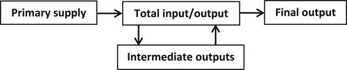
Figure 2. Common causal structure of the supply-driven IO price and quantity model.

The duality of the two Leontief models may be illustrated by post-multiplying (2) with total final demand $\mathbf{\text{y}}$. This gives: (3) ${\mathbf{\text{p}}}^{\mathrm{\prime }}\mathbf{\text{y}}={{\mathbf{\text{p}}}^{\mathrm{\prime }}}_v\mathbf{\text{C}}\mathbf{\text{L}}\mathbf{\text{y}}={{\mathbf{\text{p}}}^{\mathrm{\prime }}}_v\mathbf{\text{v}}$(3) Although the values of the solutions of (1) and (2) are linked in (3), the variables of both models move independently. Exogenous final demand quantities $\mathbf{\text{y}}$ backwardly determine primary input quantities $\mathbf{\text{v}}$ in the quantity model, whereas exogenous primary supply prices ${\mathbf{\text{p}}}_v$ forwardly determine final output prices $\mathbf{\text{p}}$ in the price model.

On to the mirror images in the second pair of basic IO models. The supply-driven IO quantity model, along the columns of Table 1, at constant unit prices, assumes that the exogenous supply of primary input quantities ${\mathbf{\text{v}}}^{\mathrm{\prime }}={\mathbf{\text{i}}}^{\mathrm{\prime }}\mathbf{\text{V}}$, along with the endogenous supply of intermediate input quantities ${\mathbf{\text{i}}}^{\mathrm{\prime }}\mathbf{\text{Z}}$, determines the size of total input, and thus of total output, i.e. ${\mathbf{\text{x}}}^{\mathrm{\prime }}={\mathbf{\text{i}}}^{\mathrm{\prime }}\mathbf{\text{Z}}+{\mathbf{\text{v}}}^{\mathrm{\prime }}$. In turn, the supply of total output, forwardly along the rows of the IOT, determines intermediate and final outputs by means of fixed intermediate output coefficients $z_{\mathrm{ij}}=x_i{b}_{\mathrm{ij}}\in {\mathbf{\text{i}}}^{\mathrm{\prime }}\mathbf{\text{Z}}={\mathbf{\text{x}}}^{\mathrm{\prime }}\mathbf{\text{B}}$ and fixed final output coefficients $y_{\mathrm{iq}}=x_i{d}_{\mathrm{iq}}\in {\mathbf{\text{i}}}^{\mathrm{\prime }}\mathbf{\text{Y}}={\mathbf{\text{x}}}^{\mathrm{\prime }}\mathbf{\text{D}}$, with $\mathbf{\text{B}}\mathbf{\text{i}}+\mathbf{\text{D}}\mathbf{\text{i}}=\mathbf{\text{i}}$. The changes in intermediate outputs subsequently lead to further and further forward changes in total input and thus in total output (see Figure 2). The solutions for total input/output, intermediate output and final output (i.e. domestic final demand and exports) then, respectively, read as follows: (4) ${\mathbf{\text{x}}}^{\mathrm{\prime }}={\mathbf{\text{x}}}^{\mathrm{\prime }}\mathbf{\text{B}}+{\mathbf{\text{v}}}^{\mathrm{\prime }}\Rightarrow {\mathbf{\text{x}}}^{\mathrm{\prime }}={\mathbf{\text{v}}}^{\mathrm{\prime }}(\mathbf{\text{I}}-\mathbf{\text{B}}{)}^{-1}={\mathbf{\text{v}}}^{\mathrm{\prime }}\mathbf{\text{G}},{\mathbf{\text{i}}}^{\mathrm{\prime }}\mathbf{\text{Z}}={\mathbf{\text{v}}}^{\mathrm{\prime }}\mathbf{\text{G}}\mathbf{\text{B}}\text{and}{\mathbf{\text{i}}}^{\mathrm{\prime }}\mathbf{\text{Y}}={\mathbf{\text{v}}}^{\mathrm{\prime }}\mathbf{\text{G}}\mathbf{\text{D}}$(4) where $\mathbf{\text{G}}$ = the Ghosh-inverse. The assumption of a single homogenous input per column of the IOT, which is hidden in (4), implies the perfect substitutability of all inputs. This makes the model highly implausible, as it allows factories to work without labor and cars to drive without gas (see further Oosterhaven, 1988).³

In the revenue-pull price dual of this model, along the rows of the IOT, at constant quantities, exogenous prices for the single homogeneous final demands of category q, $p_q\in {\mathbf{\text{p}}}_{y^{\mathrm{\prime }}}$, along with endogenous prices for the single homogenous intermediate demands of industry j, $p_j\in {\mathbf{\text{p}}}^{\mathrm{\prime }}$, weighted with their respective revenue shares $\mathbf{\text{D}}$ and $\mathbf{\text{B}}$, determine total output prices $p_i={\sum }_j{b}_{\mathrm{ij}}{p}_j+{\sum }_q{d}_{\mathrm{iq}}{p}_q\in \mathbf{\text{p}}=\mathbf{\text{B}}\mathbf{\text{p}}+\mathbf{\text{D}}{\mathbf{\text{p}}}_{y^{\mathrm{\prime }}}$ and thus total revenue. In turn, any change in total revenue is fully passed on backwardly into the single price of intermediate and primary inputs per column of the IOT, with the intermediate input price changes subsequently being passed on further and further (see Figure 1). The solution for the prices of total output/input then reads as follows: (5) $\mathbf{\text{p}}=\mathbf{\text{B}}\mathbf{\text{p}}+\mathbf{\text{D}}{\mathbf{\text{p}}}_{y^{\mathrm{\prime }}}\Rightarrow \mathbf{\text{p}}=(\mathbf{\text{I}}-\mathbf{\text{B}}{)}^{-1}\mathbf{\text{D}}{\mathbf{\text{p}}}_{y^{\mathrm{\prime }}}=\mathbf{\text{G}}\mathbf{\text{D}}{\mathbf{\text{p}}}_{y^{\mathrm{\prime }}}$(5) Obviously, at constant quantities, this model is suited to simulate the further backward, demand-driven price impacts of e.g. an increase in the export prices of particular industries. More generally, it is able to simulate any demand-driven inflation process.

The duality of these last two basic IO models may be illustrated by pre-multiplying (5) with total primary input ${\mathbf{\text{v}}}^{\mathrm{\prime }}$: (6) ${\mathbf{\text{v}}}^{\mathrm{\prime }}\mathbf{\text{p}}={\mathbf{\text{v}}}^{\mathrm{\prime }}\mathbf{\text{G}}\mathbf{\text{D}}{\mathbf{\text{p}}}_{y^{\mathrm{\prime }}}={\mathbf{\text{y}}}^{\mathrm{\prime }}{\mathbf{\text{p}}}_{y^{\mathrm{\prime }}}$(6) Again both model solutions (4) and (5) are linked by their values in (6), whereas their variables move independently: with exogenous primary supply quantities ${\mathbf{\text{v}}}^{\mathrm{\prime }}$ forwardly determining the quantities of final output ${\mathbf{\text{y}}}^{\mathrm{\prime }}$, and exogenous final output prices ${\mathbf{\text{p}}}_{y^{\mathrm{\prime }}}$ backwardly determining the prices of primary inputs $\mathbf{\text{p}}$.

3. Turning both quantity models into price models measured in values

The above-explained supply-driven IO quantity model may be re-interpreted as the cost-push IO price model measured in value terms, instead of in prices (Dietzenbacher, 1997). The economic logic of this re-interpretation follows from Figure 2 that summarizes the identical causal structure of both supply-driven models. In the Ghosh quantity model, the exogenous quantity of primary inputs initiates a forward causal chain of quantity changes along the arrows of Figure 2, whereas in the case of the Leontief price model the exogenous price of primary inputs initiates a similar forward casual chain of price changes along the same arrows.

The mathematical proof of the equivalence is simple. Substitute $\mathbf{\text{A}}=\mathbf{\text{Z}}{\widehat{\mathbf{\text{x}}}}^{-1}=\widehat{\mathbf{\text{x}}}\mathbf{\text{B}}{\widehat{\mathbf{\text{x}}}}^{-1}$ into the Leontief price model (2) and post-multiply the result with $\widehat{\mathbf{\text{x}}}$, where $\widehat{\mathbf{\text{x}}}$ = a matrix with $\mathbf{\text{x}}$ on its diagonal and zerós elsewhere. This gives: (7) ${\mathbf{\text{p}}}^{\mathrm{\prime }}\widehat{\mathbf{\text{x}}}={\mathbf{\text{p}}}^{\mathrm{\prime }}\widehat{\mathbf{\text{x}}}\mathbf{\text{B}}{\widehat{\mathbf{\text{x}}}}^{-1}\widehat{\mathbf{\text{x}}}+{{\mathbf{\text{p}}}^{\mathrm{\prime }}}_v\mathbf{\text{C}}\widehat{\mathbf{\text{x}}}$(7) Next, substitute $\mathbf{\text{V}}=\mathbf{\text{C}}\widehat{\mathbf{\text{x}}}$ in (7), and simplify and solve the result as follows: (8) ${\mathbf{\text{p}}}^{\mathrm{\prime }}\widehat{\mathbf{\text{x}}}={\mathbf{\text{p}}}^{\mathrm{\prime }}\widehat{\mathbf{\text{x}}}\mathbf{\text{B}}+{{\mathbf{\text{p}}}^{\mathrm{\prime }}}_v\mathbf{\text{V}}\Rightarrow {\mathbf{\text{p}}}^{\mathrm{\prime }}\widehat{\mathbf{\text{x}}}={{\mathbf{\text{p}}}^{\mathrm{\prime }}}_v\mathbf{\text{V}}(\mathbf{\text{I}}-\mathbf{\text{B}}{)}^{-1}$(8) Equation 8 shows that the Leontief price model (2) is identical to the Ghosh quantity model (4), except that the quantities of (4) are replaced with their corresponding values ${\mathbf{\text{p}}}^{\mathrm{\prime }}\widehat{\mathbf{\text{x}}}$ and ${{\mathbf{\text{p}}}^{\mathrm{\prime }}}_v\mathbf{\text{V}}$ in (8). ⁴

The economic logic of the comparable re-interpretation of the demand-driven IO quantity model (1) as the revenue-pull IO price model (5) measured in values, instead of in prices, follows from the common causal structure of the two models (see Figure 1). In both demand-driven models, any change in exogenous final demand, irrespective of whether it regards a price change or a quantity change, leads to a direct change in total output. Next, any change in total output backwardly leads to changes in both intermediate and primary inputs, again with the quantities changing in the quantity model and the prices changing in the price model. Finally, any change in intermediate inputs, in turn, leads to further and further backward changes in total output.

Mathematically, the equivalence follows from substituting $\mathbf{\text{B}}={\widehat{\mathbf{\text{x}}}}^{-1}\mathbf{\text{Z}}={\widehat{\mathbf{\text{x}}}}^{-1}\mathbf{\text{A}}\widehat{\mathbf{\text{x}}}$ into the revenue-pull price model (5). Pre-multiplying the result with $\widehat{\mathbf{\text{x}}}$ gives: (9) $\widehat{\mathbf{\text{x}}}\mathbf{\text{p}}=\widehat{\mathbf{\text{x}}}{\widehat{\mathbf{\text{x}}}}^{-1}\mathbf{\text{A}}\widehat{\mathbf{\text{x}}}\mathbf{\text{p}}+\widehat{\mathbf{\text{x}}}\mathbf{\text{D}}{\mathbf{\text{p}}}_{y^{\mathrm{\prime }}}$(9) Next, $\mathbf{\text{Y}}=\widehat{\mathbf{\text{x}}}\mathbf{\text{D}}$ is substituted into (7), and the result is simplified and solved as follows: (10) $\widehat{\mathbf{\text{x}}}\mathbf{\text{p}}=\mathbf{\text{A}}\widehat{\mathbf{\text{x}}}\mathbf{\text{p}}+\mathbf{\text{Y}}{\mathbf{\text{p}}}_{y^{\mathrm{\prime }}}\Rightarrow \widehat{\mathbf{\text{x}}}\mathbf{\text{p}}=(\mathbf{\text{I}}-\mathbf{\text{A}}{)}^{-1}\mathbf{\text{Y}}{\mathbf{\text{p}}}_{y^{\mathrm{\prime }}}$(10) Equation 10 shows that the Leontief quantity model (1) may indeed be interpreted as the revenue-pull price model (5) wherein the price changes are evaluated in terms of the changes in value that accompany them, i.e. with $\widehat{\mathbf{\text{x}}}\mathbf{\text{p}}$ and $\mathbf{\text{Y}}{\mathbf{\text{p}}}_{y^{\mathrm{\prime }}}$.

Note that the exogenous final output prices in (5) and (10) are defined per column of final output. In empirical applications of (5) and (10), however, it will often be more useful to assume that the prices of the cells of $\mathbf{\text{Y}}$move independently, e.g. because export price changes of food products will be different from those of chemicals. Note that this does not change the working of the model as final output prices are exogenous. If that more realistic assumption is applied to all the cells of $\mathbf{\text{Y}}$ in Figure 1, (5) and (10) change into: (5alt) $\begin{array}{rl}\mathbf{\text{p}}& =(\mathbf{\text{I}}-\mathbf{\text{B}}{)}^{-1}(\mathbf{\text{D}}\otimes {\mathbf{\text{P}}}_y)\mathbf{\text{i}}\text{and}\end{array}$(5alt) (10alt) $\begin{array}{rl}\widehat{\mathbf{\text{x}}}\mathbf{\text{p}}& =(\mathbf{\text{I}}-\mathbf{\text{A}}{)}^{-1}(\mathbf{\text{Y}}\otimes {\mathbf{\text{P}}}_y)\mathbf{\text{i}},\end{array}$(10alt) respectively, where $\otimes$ = the cell x cell multiplication of two matrices, and $p_{\mathrm{iq}}\in {\mathbf{\text{P}}}_y$ = the matrix with exogenous final output prices. In contrast to (5) and (10), (5alt) and (10alt) allow for an evaluation of the different backward impacts of a 10% increase in the export price of crude oil compared to a 10% increase in the export price of food products; with (5alt) showing the relative backward impact on total output prices and (10alt) showing the corresponding absolute backward impact in terms of changes in the values of total output due to the price change at hand. Dividing the new values by the base year values of (10alt) also gives the relative price changes.

4. Ultimate input–output equations

Before concluding, it is worthwhile to look further at the price re-interpretations of both quantity models, as each combines the solutions of the two corresponding basic IO models, which is why we may call them the ultimate input–output equations.

First, reconsider the solution of the re-interpretation of the Ghosh quantity model as the Leontief price model measured in values instead of in prices, which is derived in (8): (11) ${\mathbf{\text{p}}}^{\mathrm{\prime }}\widehat{\mathbf{\text{x}}}={{\mathbf{\text{p}}}^{\mathrm{\prime }}}_v\mathbf{\text{V}}(\mathbf{\text{I}}-\mathbf{\text{B}}{)}^{-1}$(11) Obviously, we may label (11) the ultimate supply-driven IO equation, as it nicely combines the solution of the supply-driven quantity model and the supply-driven price model.

If the quantities V and x are kept constant, (11) shows the impact of changing primary input prices on the prices of total input/output in terms of the absolute changes in the corresponding values, instead of in terms of the changes in the prices as in (2). Dividing the new values by the base year values gives the relative changes in all exogenous and endogenous prices.

Alternatively, if the prices ${\mathbf{\text{p}}}_v$ and p are kept constant at their base year values of one, (11) gives the impact of changing quantities of primary inputs on the quantities of total input/output according to the highly implausible supply-driven IO quantity model. Dividing the new values by the base year values gives the relative changes in total output.

Subsequently, to get the changes in endogenous final output quantities and ditto prices (11) needs to be post-multiplied with the final output coefficients' matrix D. This delivers the ultimate IO equation for endogenous final outputs: (12) ${\mathbf{\text{p}}}^{\mathrm{\prime }}\mathbf{\text{Y}}={{\mathbf{\text{p}}}^{\mathrm{\prime }}}_v\mathbf{\text{V}}(\mathbf{\text{I}}-\mathbf{\text{B}}{)}^{-1}\mathbf{\text{D}}$(12) Keeping the prices ${\mathbf{\text{p}}}_v$ and p constant in (12) delivers the changes in the quantities of final output according to the Ghosh quantity model, whereas keeping the quantities V and Y constant in (12) delivers the changes in the (final) output prices according to the Leontief price model, as measured by the absolute changes in the corresponding values. Dividing by the base year values of one gives the relative price changes.⁵

Second, reconsider the solution of the re-interpretation of the Leontief quantity model as the Davar/Oosterhaven price model measured in values instead of in prices, as derived in (10): (13) $\widehat{\mathbf{\text{x}}}\mathbf{\text{p}}=(\mathbf{\text{I}}-\mathbf{\text{A}}{)}^{-1}\mathbf{\text{Y}}{\mathbf{\text{p}}}_{y^{\mathrm{\prime }}}$(13) Obviously, we may label (13) the ultimate demand-driven IO equation, as it combines the solutions of the demand-driven price and quantity models.

If the prices ${\mathbf{\text{p}}}_{y^{\mathrm{\prime }}}$ and p are kept constant at their base year values of one, (13) gives the impact of absolute changes in the quantities of final demand on the quantities of total output according to the Leontief quantity model. Again, dividing the new values by the base year values gives the relative changes in the quantities of total output.

Alternatively, holding the quantities Y and x constant, (13) gives the impact of changes in final output prices on the prices of total output according to the revenue-pull IO price model, but measured in terms of the effect on the corresponding absolute values, instead of in terms of prices as in (5). Again, dividing the new values by the old values gives the relative changes in all exogenous and endogenous prices.

Subsequently, to get the changes in the endogenous primary input quantities and ditto prices, (13) needs to be pre-multiplied with the primary input coefficients' matrix C. This delivers the ultimate IO equation for endogenous primary inputs: (14) $\mathbf{\text{V}}\mathbf{\text{p}}=\mathbf{\text{C}}(\mathbf{\text{I}}-\mathbf{\text{A}}{)}^{-1}\mathbf{\text{Y}}{\mathbf{\text{p}}}_{y^{\mathrm{\prime }}}$(14) Keeping prices ${\mathbf{\text{p}}}_{y^{\mathrm{\prime }}}$ and p constant in (14) gives the changes in the quantities of primary inputs according to the Leontief quantity model, whereas keeping the quantities Y and V constant in (14) gives the changes in the (primary) input prices according to the Davar/Oosterhaven price model, as measured by the corresponding values of primary inputs. Dividing by the base year values again delivers the relative price changes.⁶

5. Conclusion

This note reiterates and elegantly proves that the supply-driven input–output (IO) quantity model of Ghosh (1958) may be re-interpreted as the cost-push IO price model of Leontief (1951), but measured in value terms instead of in prices (Dietzenbacher, 1997). Additionally, it proves that the demand-driven IO quantity model of Leontief (1941) may similarly be re-interpreted as the almost unknown revenue-pull IO price model (Davar, 1989; Oosterhaven, 1989), again measured in value terms instead of in prices. Furthermore, it shows that the solution of the supply-driven quantity model may be combined in the single Equation 11 with that of the cost-push price model in what may be called: the ultimate supply-driven IO equation. Similarly, it is shown that the solution of the demand-driven quantity model may be combined in the single Equation 13 with that of the revenue-pull price model in what may be called: the ultimate demand-driven IO equation.

The new price interpretation of the Leontief quantity model opens up hitherto unused opportunities to do all kinds of demand-driven inflation simulations of exogenous final output price changes. These may be done with the basic Leontief model, but of course also with extensions of this basic model. Interregional and international extensions would allow for simulations of demand-driven, backward price impacts along interregional and international interindustry supply chains, while extensions with endogenous household expenditures would allow for simulations of demand-driven interindustry price-wage-price spirals (see Oosterhaven, 2022, Ch. 7, for a combination of these two model extensions in case of the supply-driven inflation model). These are just two examples of the many possible applications of the price re-interpretation of the Leontief quantity model.

Disclosure statement

No potential conflict of interest was reported by the author(s).

Notes

1 An alternative interpretation in which the Ghosh model is not the exact opposite of the Leontief model is presented by Mesnard (2009). His point of departure is a physical IO table that has homogeneous outputs along its rows and heterogeneous inputs along its columns. With this asymmetric base assumption naturally only asymmetric results can be derived. However, even tons of steel have different qualities with different prices, which is why they cannot sensibly be added in physical units. In real life, any IOT will have heterogeneous outputs along its rows as well as heterogeneous inputs along its columns, which is our point of departure, naturally leading to symmetric results.

2 Note that (2) uses the standard theoretical IO assumption that the prices of the primary inputs are uniform across the corresponding rows. In empirical applications, however, it is often more useful to assume that price changes may be different along the rows of the primary inputs, e.g. because import price changes will be different for different products. This does not change the working of the model, as these prices are exogenous. See Przybyliński and Gorzałczyński (2022) for a recent application of this model. See (5alt) and (10alt) for the analogous modification of the demand-driven price model.

3 See Gruver (1989) and Rose and Allision (1989) for attempts to defend the Ghosh quantity model, and Oosterhaven (1989) for a rebuff. After this exchange the Ghosh quantity model has hardly been used anymore. See Guerra and Sancho (2011) for an attempt to rescue the Type II Ghosh model in case of centrally planned economies, and Oosterhaven (2012) for a rebuff. In an otherwise fine article (Rose et al., 2018), it was recently suggested that the plausibility of the Ghosh quantity model should be evaluated more positively in case of negative supply shocks, such as disasters, as opposed to positive supply shocks. Oosterhaven (2022, Ch. 7 & 8) shows that there is no foundation for this distinction.

4 Note that Dietzenbacher (1997), after showing that the original Ghosh quantity model (4) may be re-interpreted as the Leontief price model, renamed (4) the Ghosh price model, and renamed the price interpretation of Leontief's model (10) the Ghosh quantity model. This unfortunate choice of terminology leads to defining away two of the four basic IO models, namely the original Ghosh quantity model (4) as well as its dual price model (5), as may e.g. be observed in Rueda-Cantuche (2011) and Miller and Blair (2022, p. 301).

5 Note that (11) also gives the solution of the supply-driven IO model with fixed value output coefficients. This model has not yet been formulated. It may be based on the assumption that the ratio of the values of intermediate output to total input $b_{\mathrm{ij}}=(z_{\mathrm{ij}}{p}_j)/(x_i{p}_i)$ is fixed. This model is of little direct use as it is underdetermined, i.e. it has more unknown price and quantity variables (i.e. 2 x I) than it has equations (i.e. I).

6 Note that (14) also gives the solution to the demand-driven IO model with fixed value input coefficients (see de Boer, 1976, for a discussion). This model is based on the assumption that the ratio of the values of intermediate input to total output $a_{\mathrm{ij}}=(p_i{z}_{\mathrm{ij}})/(p_j{x}_j)$ is constant. This model is of little direct use as it is underdetermined, just as the supply-driven IO model with fixed value output coefficients.

Appendix. Assumptions and solutions of the four basic input–output models.

Table

Demand-driven quantity & cost-push price model:	Supply-driven quantity & revenue-pull price model:
For the individual firm:
given demand for its single homogeneous output i.e. perfect substitution among all outputs full complementarity of all inputs (fixed input ratios) cost minimization at given input prices derived demand for inputs (backward linkages) full competition, i.e. forward passing on of all input price changes into the single output price	given supply of its single homogeneous input, i.e. perfect substitution among all inputs perfect jointness of all outputs (fixed output ratios) revenue maximization at given output prices derived supply of outputs (forward linkages) full competition, i.e. backward passing on of all output price changes into the single input price
For the economy as a whole:
exogenous demand for final outputs per industry endogenous demand for all inputs per industry perfectly elastic supply of all primary inputs, i.e. exogenous primary input prices endogenous total output prices and quantities	exogenous supply of primary inputs per industry endogenous supply of all outputs per industry perfectly elastic demand for all final outputs, i.e. exogenous final output prices endogenous total input prices and quantities
Solution of the two Leontief models:	Solution of the two Ghosh models:
$\mathbf{v}=\mathbf{C}(\mathbf{I}-\mathbf{A}{)}^{-1}\mathbf{y}$, with $\mathbf{y}=\mathbf{Y}\mathbf{i}$ and $\mathbf{v}=\mathbf{V}\mathbf{i}$ ${{\mathbf{p}}^{\mathrm{\prime }}}_y={\mathbf{p}}^{\mathrm{\prime }}={{\mathbf{p}}^{\mathrm{\prime }}}_v\mathbf{C}(\mathbf{I}-\mathbf{A}{)}^{-1}$	${\mathbf{y}}^{\mathrm{\prime }}={\mathbf{v}}^{\mathrm{\prime }}(\mathbf{I}-\mathbf{B}{)}^{-1}\mathbf{D}$, with ${\mathbf{y}}^{\mathrm{\prime }}={\mathbf{i}}^{\mathrm{\prime }}\mathbf{Y}$ and ${\mathbf{v}}^{\mathrm{\prime }}={\mathbf{i}}^{\mathrm{\prime }}\mathbf{V}$ ${\mathbf{p}}_{v^{\mathrm{\prime }}}=\mathbf{p}=(\mathbf{I}-\mathbf{B}{)}^{-1}\mathbf{D}{\mathbf{p}}_{y^{\mathrm{\prime }}}$

Source: Oosterhaven (1989 and 2022, Ch. 7).

References

- Boer, P. C. M. de. (1976). On the relationship between production functions and input–output analysis with fixed value shares. Weltwirtschaftliches Archiv, 112(4), 754–759. https://doi.org/10.1007/BF02705985
- Davar, E. (1989). Input–output and general equilibrium. Economic Systems Research, 1(3), 331–344. https://doi.org/10.1080/09535318900000022
- Dietzenbacher, E. (1997). In vindication of the Ghosh model: A reinterpretation as a price model. Journal of Regional Science, 37(4), 629–651. https://doi.org/10.1111/0022-4146.00073
- Ghosh, A. (1958). Input–output approach in an allocation system. Economica, 25(4), 58–64. https://doi.org/10.2307/2550694
- Gruver, G. W. (1989). On the plausibility of the supply-driven input–output model: A theoretical basis for input-coefficient change. Journal of Regional Science, 29(3), 441–450. https://doi.org/10.1111/j.1467-9787.1989.tb01389.x
- Guerra, A.-I., & Sancho, F. (2011). Revisiting the original Ghosh model: Can it be made more plausible? Economic Systems Research, 23(3), 319–328. https://doi.org/10.1080/09535314.2011.566261
- Leontief, W. W. (1941). The structure of the American economy, 1919-1929: An empirical application of equilibrium analysis. Cambridge University Press.
- Leontief, W. W. (1951). The structure of the American economy: 1919-1939, 2nd edn. Oxford University Press.
- Mesnard, L. de. (2009). Is the Ghosh model interesting? Journal of Regional Science, 49(2), 361–372. https://doi.org/10.1111/j.1467-9787.2008.00593.x
- Miller, R. E., & Blair, P. D. (2022). Input–output analysis, foundations and extensions, Third edition. Cambridge University Press.
- Oosterhaven, J. (1988). On the plausibility of the supply-driven input–output model. Journal of Regional Science, 28(2), 203–217. https://doi.org/10.1111/j.1467-9787.1988.tb01208.x
- Oosterhaven, J. (1989). The supply-driven input–output model: A new interpretation but still implausible. Journal of Regional Science, 29(3), 459–465. https://doi.org/10.1111/j.1467-9787.1989.tb01391.x
- Oosterhaven, J. (2012). Adding supply-driven consumption makes the Ghosh model even more implausible. Economic Systems Research, 24(1), 101–111. https://doi.org/10.1080/09535314.2011.635137
- Oosterhaven, J. (2022). Rethinking input–output analysis, a spatial perspective, Second edition. Advances in Spatial Science. Springer.
- Przybyliński, M., & Gorzałczyński, A. (2022). Applying the input–output price model to identify inflation processes. Journal of Economic Structures, 11(1), https://doi.org/10.1186/s40008-022-00264-w
- Rose, A., & Allision, T. (1989). On the plausibility of the supply-driven input–output model: Empirical evidence on joint stability. Journal of Regional Science, 29(3), 451–458. https://doi.org/10.1111/j.1467-9787.1989.tb01390.x
- Rose, A., Wei, D., & Paul, D. (2018). Economic consequences of and resilience to a disruption of petroleum trade: The role of seaports in U.S. energy security. Energy Policy, 115, 584–615. https://doi.org/10.1016/j.enpol.2017.12.052
- Rueda-Cantuche, J. M. (2011). The choice of type of input–output table revisited: Moving towards the use of supply-use tables in impact analysis. Statistics and Operations Research Transactions, 35(1), 21–38.