Improving visualisation and prediction performance of supervised self-organising map by modified contradiction resolution

Abstract

We have previously proposed a new type of information-theoretic method where a neuron is evaluated by itself (self-evaluation) and by its surrounding neurons (outer-evaluation). If contradiction between different types of evaluation exists, it is reduced as much as possible. In the present paper, we try to separate self- and outer-evaluation more explicitly and introduce the importance of neurons. First, we separate self- and outer-evaluation to enhance the characteristics shared by the two types of evaluation. Second, we introduce the importance of neurons in evaluation. By using a limited number of important neurons in evaluation, we expect the main characteristics in input patterns to emerge. We applied this contradiction resolution to two types of data, namely, the Senate data and the Euro-yen exchange rates. In both data sets, experimental results confirmed that improved prediction performance was obtained. Prediction performance was better than that obtained by the conventional self-organising map (SOM) and radial basis function networks. In addition, final representations obtained by contradiction resolution were easier to interpret than those given by the conventional SOM. Experimental results confirmed that improved interpretation and visualisation were accompanied by improved prediction performance.

Keywords:

• SOM
• contradiction resolution
• visualisation
• prediction
• class structure

1. Introduction

1.1. Class structure clarification in self-organising maps

We have previously introduced contradiction resolution (Kamimura, 2012a, 2012b, 2012c) to show the importance of multiple points of view for neurons. Contradiction resolution is in particular introduced to clarify the class or cluster structure of self-organising maps (SOMs) (Kohonen, 1988; Kohonen, 1990; Kohonen, 1995). The SOM has been extensively used for data visualisation and the clarification of class structure in input patterns. In the SOM, after competition among neurons a winning neuron is selected (competition), and this winning neuron cooperates with the surrounding neurons (cooperation). The surrounding neurons tend to fire according to their distance from this winning neuron. Usually, the range of cooperation between neurons is wide at the beginning and shrinks gradually to keep topological preservation in the output space. In the SOM, topological consistency and continuity are considered to be very important, and a number of evaluation measures have been proposed (Bauer & Pawelzik, 1992; Kaski et al., 2003; Kiviluoto, 1996; Lee & Verleysen, 2008; Merényi et al., 2009; Polzlbauer, 2004; Tasdemir & Merényi, 2009; Venna & Kaski, 2001; Villmann et al., 1997). Thus, to improve topological consistency, it takes long learning processes to adjust neurons in the cooperation process.

However, the importance of topological preservation in SOM has made it difficult to interpret connection weights and neurons’ outputs produced by SOM, which is called ‘SOM knowledge’ in this paper. Though SOM has a good reputation for visualisation, it is ironically difficult to visualise class structure when the SOM is applied to the detection of class structure or class boundaries. Thus, many different kinds of visualisation and interpretation methods have been developed (De Runz et al., 2012; Kaski et al., 1998; Mao & Jain, 1995; Shieh & Liao, 2012; Su & Chang, 2001; Vesanto, 1999; Wu & Chow, 2005; Xu et al., 2010; Xu et al., 2011; Xu & Chow, 2011; Yin, 2002), to cite a few. Despite the abundance of available methods, we still have difficulty in interpreting and visualising the results obtained by SOM.

We believe that focusing on topological consistency, the uniform occurrence of neurons, the uniform coverage of data, and uniform approximation of probability distribution coverage of the data space (DeSieno, 1988; Ridella et al., 2001; Van Hulle, 1996; Van Hulle, 1997; Van Hulle, 1999; Van Hulle, 2004) in the SOMs have made it impossible to interpret SOM knowledge. This is because those properties tend to hide discontinuity or drastic change in outputs, weights, and class boundaries in particular. Thus, it is important for the sake of the interpretation of SOM knowledge to create more interpretable representations, even if they violate topological consistency (Merenyi & Jain, 2004; Merenyi et al., 2007; Merényi et al., 2009; Villmann & Claussen, 2006).

1.2. Two problems of contradiction resolution

To clarify class structure, we need to separate characteristics due to the individuality and collectivity of neurons. This is because the class boundary is a place where individual neurons behave differently from other neighbouring neurons. Thus, we have introduced the ‘contradiction resolution’ method to separate those characteristics (Kamimura, 2012a, 2012b, 2012c). To distinguish between the characteristics of individual and collective neurons, we have introduced the concept of ‘self-evaluation’ and ‘outer-evaluation’. In contradiction resolution, ‘evaluation’ is considered to be the process of obtaining neurons’ outputs. In self-evaluation, a neuron's output is computed by using connection weights into the neuron and the corresponding input pattern. On the other hand, in outer-evaluation, a neuron's output is computed by considering the outputs from all neighbouring neurons. The introduction of difference between the two types of evaluation enhances the characteristics shared by them, and consequently those not shared by the two types of evaluation are also clarified.

In contradiction resolution, the separation of self- and outer-evaluation plays a key role. However, we have not fully succeeded in the separation (Kamimura, 2012a). Results from the self-evaluation could not clearly be separated from those by the outer-evaluation because the outer-evaluation was influenced by the self-evaluation. Thus, the explicit separation of self-evaluation from outer-evaluation is needed to formulate contradiction between self- and outer-evaluation. In the present model, we try to separate self-evaluation from outer evaluation by deleting the effect of self-evaluation from the result by outer-evaluation.

Second, the importance of neurons is considered. In previous work on contradiction resolution (Kamimura, 2012a), a neuron was evaluated by multiple neurons surrounding a neuron. In particular, in the previous model (Kamimura, 2012a), a neuron was evaluated by all its surrounding neurons. In the present model, we suppose competition among neurons and a limited number of winning or important neurons which can participate in the evaluation. We expect that by using a limited number of winning or important neurons, the most important characteristics can be clarified. This is because when using all surrounding neurons, the characteristics to be extracted may be weakened by the effect of unimportant neurons.

1.3. Outline

In Section 2, we first explain the concept of contradiction resolution between self- and outer-evaluation. We try to explain how to separate self- and outer-evaluation. Then, we explain how to compute winning neurons and how to evaluate a neuron by a limited number of winning neurons. Next, we explain how to implement contradiction resolution and how to reduce the contradiction in terms of the Kullback–Leibler divergence. We present three experimental results, namely, the Senate data and the Euro-yen exchange rates with small- and large-sized networks. In all the data, we try to show that improved prediction performance was obtained by changing the number of winners for evaluation. The prediction performance was better than that obtained by the conventional SOM and radial basis function (RBF) networks with a limited number of winning neurons. In addition, the internal representations obtained by our method were much easier to interpret than those by the conventional SOM.

2. Theory and computational methods

2.1. Two types of evaluation

Contradiction resolution lies in the perception and resolution of contradiction where we distinguish two types of evaluation, namely, self- and outer-evaluation. Self-evaluation is a process of producing a neuron's output only considering connection weights to the neuron and the corresponding input patterns. This means that the outputs from the neurons are computed by themselves. On the other hand, in the outer-evaluation, a neuron's output is determined by computing the effects of all surrounding neurons.

Let us explain how to evaluate outputs from neurons. Figure 1 shows the network architecture used in this paper. First, we have input and competitive neurons in the competitive layer. Connection weights in this layer self-organise by contradiction resolution. In addition, we have an output layer in which connection weighs are updated to reduce the difference between targets and outputs by the RBF network.

Figure 1. Network architecture for supervised SOM.

Now, the sth input pattern of total S patterns can be represented by . Connection weights into the jth competitive unit of total M units are computed by . Now we can compute the outputs obtained through self- and outer-evaluation. A neuron's outputs can be computed by using the outputs from the same neuron. This process is called ‘self-evaluation’. Then, the jth competitive neuron output without considering the other neurons can be computed by

where and are supposed to represent L-dimensional input and weight column vectors, where L denotes the number of input units. The spread parameter is defined by

where β is larger than zero. When the parameter β increases, the corresponding spread parameter decreases. The firing probabilities by self-evaluation are computed by

Outer-evaluation is a process of computing the outputs by considering all neighbouring neurons’ outputs. We approximate the outputs by summing the outputs of all neighbouring neurons weighted by the relations between them. Then, the outputs by the outer evaluation are defined by

where φ_jm denotes relations between the jth and mth neuron. Following the formulation of SOM, we used the neighbourhood function

where and denote the position of the jth and the mth neuron on the output space and is a spread parameter. The output obtained by this evaluation is the sum of all neighbouring neurons’ outputs rates weighted by the relations between them. Then, the firing probabilities by the outer-evaluation are computed by

2.2. Separation of self and outer-evaluation

We have defined the output obtained through the outer-evaluation as the weighted sum of all neighbouring neurons, including the output of the neuron, namely,

The output from the outer-evaluation is the sum of the outputs from the neuron and the outputs from the other neurons. We can lay out a new definition of outer-evaluation as shown in Figure 2(b). As shown in Figure 2(a), we have so far computed a neuron's output at the centre by summing the outputs from all surrounding neurons, including the neuron itself. On the other hand, we now compute the neuron's output at the centre excluding the same neuron's output, as shown in Figure 2(b):

Figure 2. Outer-evaluation by the previous (a) and the present (b) method.

2.3. Limited evaluation

We have observed that in the outer-evaluation, some neurons have more important effects while others contribute almost nothing to the evaluation. Thus, we should take into account the importance of neurons and choose a limited number of important neurons in order to make the outer-evaluation more effective (Zhang et al., 2010). We here introduce limited evaluation, meaning that a neuron is evaluated using a limited number of neurons. When the sth input pattern is presented, we first determine the winner c₁

Then, based on this winner, we determine the rank of the neurons

By using this rank, we can define limited evaluation with a limited number R of neurons as shown in Figure 3. In Figure 3(a), a neuron at the centre is evaluated by all surrounding neurons. On the other hand, in Figure 3(b), a neuron's output at the centre is evaluated by the first and the second winner. Now, the output from the jth neuron is the sum of the first R winning neurons’ outputs minus the output from the jth neuron itself, if it exists among the R winning neurons,

where

The output of this evaluation is the sum of all neighbouring neurons’ outputs weighted by the relations between them except for the output of the neuron itself. Then, the firing probabilities obtained through outer-evaluation are defined by

Figure 3. Limited number of winning neurons in modified method.

2.4. Contradiction resolution

Contradiction resolution aims to reduce contradiction between self- and outer-evaluation. We use the Kullback–Leibler divergence to represent contradiction or difference between self- and outer-evaluation. Using the Kullback–Leibler divergence, contradiction with R winning neurons is defined by

where p(s) denotes the probability of occurrence of the sth input pattern and set to

In addition to this contradiction, we have other errors which must be minimised, namely quantisation errors (QEs) between connection weights and input patterns

To realise the minimum contradiction in terms of evaluation and QEs, we first try to minimise the KL divergence using fixed QEs (see Appendix). Then, we have

By substituting the optimal firing rate for p(j | s), we have

The second term of the right-hand side of the above equation is called ‘free energy’:

The free energy can be expanded into

Thus, we actually minimise the KL divergence as well as the QEs. By differentiating the free energy, we can obtain updated rules

2.5. Output layer

The output layer is trained by the supervised learning. Though any learning methods can be used for the layer (Zhang et al., 2010), we in particular used RBF, because our model is close to RBF networks. We can consider weights by our method as inputs to RBF networks. Thus, in the output layer, the method is equivalent to the RBF function network. Then, for easy understanding, we follow the notation for the RBF network. Outputs from the output layer are defined by The corresponding targets are defined by Then, we define the design matrix , whose element at the sth row and jthe column is defined by

where denotes the spread parameter. When we use the regularisation parameter λ, connection weights were computed by

where denotes the M by M identity matrix. Finally, the outputs are computed by

The model selection criteria we used was the generalised cross validation (GCV) (Golub et al., 1979; Orr, 1996). This is because the GCV has shown better performance for all the methods used in the experiments. The regularisation parameter λ was re-estimated by the re-estimation formula (Orr, 1996) with the initial values from 10⁻¹ to 10⁻¹⁰. Finally, the spread parameter was approximated by

where θ is a scaling factor. The best values for θ was chosen with initial values from 0.1 to 5 by 0.1.

2.6. Computational methods for contradiction resolution

We applied the method to the SOMs and used the neighbourhood function representing relations φ between neurons. Let us consider the following neighbourhood function that is usually used in SOMs

where and denote the position of the jth and the cth unit on the output space and is a spread parameter. In the actual learning, two parameters β and γ should be determined. The parameter can be described by

where β is greater than zero. When the parameter β is increased, the number of strongly firing neurons decreases and finally only one neuron wins the competition and fires the most strongly.

The neighbourhood range decreases as learning is advanced. By the parameter γ, we define the neighbourhood function

where γ is the number of iteration for re-estimating connection weights. The re-estimation processes terminated when mean squared error (MSE) between weights at the γth iteration and at the γ−1th iteration was less than 10⁻⁵ or the number of iterations was larger than 50. We used this exponential form, because in the actual implementation of SOM, learning is composed of the rough and fine-tuning modes (Vesanto et al., 2000b). In the rough mode, the range of the neighbourhood gradually decreases, but in the fine-tuning mode, the neighbourhood parameter is usually set to one. Finally, the spread parameter was approximated by

where θ is a scaling factor. The value for θ was always set to five and the parameter β was increased gradually.

3. Results and discussion

3.1. Senate classification

3.1.1. Experiment outline

We used the well-known Senate data where the half of data was Republicans and the other half was Democrats. The data was composed of ‘yes’ or ‘no’ for 19 votes (Romesburg, 1984). The number of congressmen was originally 12, but the number was increased to 120 by adding it the small random numbers (standard deviation=0.1). Thus, the number of training and testing patterns was 60, respectively. The optimal parameter values by the training data were obtained by the GCV.

The objective of this experiment is to show that improved prediction performance can be obtained by adjusting the number of winners or competitive neurons, and that clearer internal representation is accompanied by better prediction performance.

3.1.2. Quantitative evaluation

We evaluated the performance of our method in terms of well-known measures in neural networks since our main focus in this paper was on the easy reproduction of the results. We used the MSEs between targets and outputs on the output layer as the main measure for evaluating the performance. For the property of the SOMs, we used well-known and simple error measures for quantisation evaluation, namely, QEs and topographic errors (TEs). Naturally, there are a number of different type of errors, in particular, to measure topological preservation (Merényi et al., 2009; Tasdemir & Merényi, 2009). The reason for this choice is only the simplicity of the measure, because the QE is simply the average distance from each data vector to its BMU (best-matching unit). The TE is the percentage of data vectors for which the BMU and the second-BMU are not neighbouring units (Kiviluoto, 1996). In addition, to measure how the maps are organised, we computed mutual information (INF)

This mutual information represents the degree of organisation of a system. For example, when mutual information becomes smaller, all neurons tend to fire uniformly. When mutual information increases, neurons tend to respond very specifically to input patterns.

Table 1 shows the summary of the experimental results for the Senate data. When the parameter β increased, the number of winners increased and reached a peak of 15 neurons when the parameter β was six. Then, the number of winners decreased when the parameter β increased. The MSE fluctuated when the parameter β was small, and the lowest value of 0.053 was obtained when the parameter β was seven and the number of winners was 13. When the parameter β increased further, the MSE gradually increased again. The QE and TEs seemed to decrease when the parameter β increased. Mutual information increased when the parameter β increased. The results show that better prediction performance did not necessarily correspond to lower QE and TEs, and higher mutual information.

Table 1.  The number of winners, MSE for testing data, QE, TEs and mutual information (INF) when the parameter β was changed from one to one to 15 by the weighted evaluation for the Senate data.

β	Win	MSE	QE	TE	INF
1	4	0.072	1.367	0.483	0.347
2	9	0.091	1.482	0.000	0.209
3	9	0.109	1.463	0.017	0.239
4	5	0.096	1.387	0.267	0.371
5	5	0.075	1.372	0.083	0.388
6	15	0.100	1.433	0.167	0.338
7	13	0.053	1.413	0.133	0.412
8	12	0.072	1.414	0.133	0.439
9	9	0.089	1.365	0.000	0.462
10	9	0.087	1.210	0.000	0.513
11	1	0.131	1.032	0.250	0.588
12	7	0.132	0.967	0.000	0.692
13	2	0.167	0.949	0.000	0.693
14	9	0.138	0.757	0.000	0.835
15	2	0.154	0.923	0.000	0.757

Note: The number of winners (Win) was determined to minimise MSE.

3.1.3. Visual evaluation

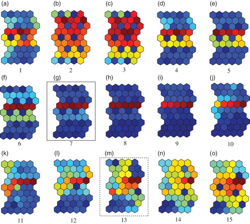
We then evaluated the performance of our method visually. Figure 4 shows the U-matrices when the parameter β increased from one to 15. The U-matrix is a popular method to visualise connection weights. The U-matrix is based on averaged distances between neighbouring neurons on the output space

When the values of the U-matrix become larger, differences between neurons also become larger. At points where larger U-matrix values exist, there is a possibility of class boundaries. In the following U-matrix figures, larger values and smaller values are represented in warmer and cooler colours. When the parameter β increased, the upper and lower sides of the matrix were clearly separated. When the MSE was its lowest in Figure 4(g), a class boundary in brown in the middle of the map appeared. The brown class boundary in the middle of the matrix clearly separated it into upper and lower parts. On the other hand, for the worst case in Figure 4(m), the U-matrix did not show any regularity.

Figure 4. U-matrices with the optimal number of winners when the parameter β was increased from one (a) to 15 (o) for the Senate data.

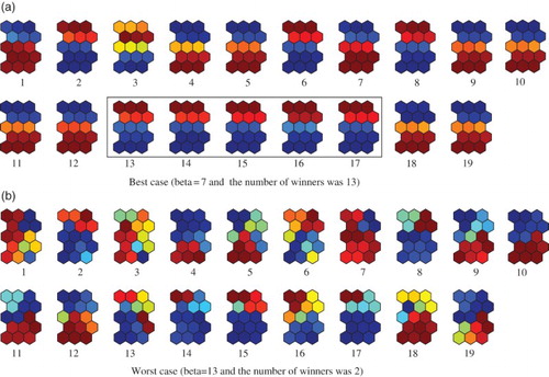
Figure 5(a) and 5(b) show connection weights w_kj for the best and worst cases in Table 1. For the best case in Figure 5(a), all connection weights were divided into upper and lower parts. In addition, we could see clear characteristics for each connection weight. For example, the variables from No.13 to No.17 showed similar characteristics in that the upper part was stronger than the lower part. We found that these five variables played critical roles in classification. On the other hand, for the worst case in Figure 5(b), a number of different types of connection weights were observed. Clear characteristics could not be obtained in the connection weights. The results show that improved prediction performance corresponded to improved visualisation.

Figure 5. Connection weights for the best case (a) and the worst case (b) in Table 1 for the Senate data.

3.1.4. Interpretation

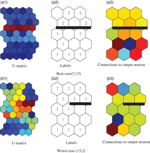
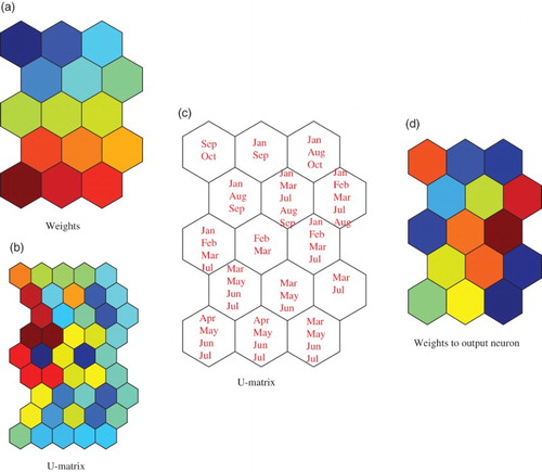
Figure 6(a) and 6(b) show connection weights from input neurons to competitive neurons (1), labels (2) and weights from competitive neurons to the output neuron (3). Connection weights from input neurons to competitive neurons in Figure 6(a1) and from competitive neurons to the output neuron in Figure 6(a3) showed clear separation of the upper and lower parts by the class boundary in the middle. The labels in Figure 6(a2) confirmed the validity of the class boundary by which Democrats were represented as ‘1’ and Republicans as ‘2’, and were clearly separated. On the other hand, for the worst case in Figure 6(b), Democrats and Republicans were not separated at all. In particular, Republicans and Democrats were mixed in the matrix of labels in Figure 6(b). The results show that better interpretation of internal representations was accompanied by improved prediction performance.

Figure 6. Weights from the first input neuron, U-matrices, labels and weights to the output neuron for the best case (a) and the worst case (b) for the Senate data. The black bars were manually added and show possible class boundaries, based on the U-matrix.

3.1.5. Using conventional methods

We applied the conventional SOM to the Senate data for comparison. For producing the SOMs, the well-known SOM toolbox of Vesanto et al. (2000a) was used, because the final results of the SOM have been very different given small changes in implementation (such as changes in initial conditions). We have confirmed the reproduction of stable final results by using this package.

Table 2 shows the summary of experimental results by the conventional SOM and RBF networks. By the conventional SOM, the MSE for testing data was 0.104. On the other hand, by contradiction resolution in Table 1, the MSE was 0.053 for the best case. In addition, there were many cases where MSE values were lower than the 0.104 obtained when using the conventional SOM. A QE of 1.161 and TE of zero were lower than those by the contradiction resolution for the best case. However, we should point out that the QE and TEs could be decreased by increasing the value of the parameter β in Table 1. By the RBF networks with feedforward selection (FS) and ridge regression (RR) (Chen et al., 1991; Orr, 1999; Orr, 1996), the MSE was 0.07, as in Table 2, which was not smaller than that by contradiction resolution in Table 1.

Table 2.  MSE for testing data, QEs, TEs and mutual information (INF) by the conventional SOM and RBF networks for the Senate data.

Size or methods	MSE	QE	TE	INF
SOM	0.104	1.161	0.000	0.426
RBF(FS)	0.070
RBF(RR)	0.070

Notes: Model selection criterion was GCV. The symbols ‘FS’ and ‘RR’ represent the forward selection and Ridge regression for the RBF networks.

Figure 7 shows the U-matrix (1), labels (2) and weights into the output neuron (3) by the conventional SOM. Class boundary in Figure 7(a), labels in Figure 7(b) and weights into the output neuron showed the upper and lower parts, but they were not clearer than those obtained by the contradiction resolution in Figure 6(a). Figure 8 shows connection weights by the conventional SOM for the Senate data. Compared weights by the contradiction resolution in Figure 5(a), clear characteristics could not be seen.

Figure 7. U-matrice (a), labels (b) and weights to output neuron (c) by the conventional SOM for the Senate data.

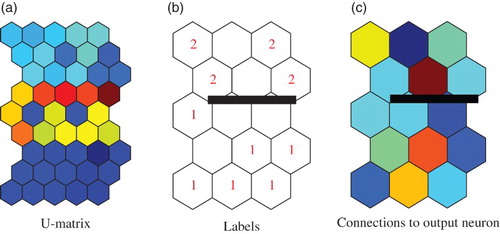
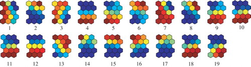
Figure 8. Connection weights by the conventional SOM for the Senate data.

3.2. Euro-Yen exchange rate prediction: experiments with small size

We tried to predict the Euro-Yen exchange rates at time t by considering the previous k rates at times t−1, t−2, …, t−k. For the Euro-Yen exchange rates, it was necessary to determine the time lag. We determined the time lag based on the errors (MSE) for the testing data. Because the results were similar for different size of networks, we used a network with 5 by 3 neurons. Table 3 shows the results for the networks. When the time lag was increased, MSE fluctuated greatly. However, we could see that when the time lag was four, the minimum MSE was obtained. The data for the exchange rates were divided into the training (⅘) and testing (⅕) data. Optimal parameter values for the training data were determined using GCV.

Table 3.  MSE for testing data, QEs, TEs and mutual information when the lag was changed from one to 10 for the 10 by 5 map.

Lag	MSE	QE	TE	INF
1	0.511	1.276	0.149	1.102
2	2.999	2.054	0.088	1.089
3	0.439	2.677	0.140	1.092
4	0.436	3.234	0.094	1.087
5	0.591	3.758	0.073	1.089
6	0.519	4.245	0.084	1.089
7	0.867	4.735	0.074	1.081
8	1.343	5.169	0.101	1.080
9	0.606	5.596	0.106	1.075
10	5.128	6.036	0.096	1.071

3.2.1. Prediction performance

Table 4 shows the summary of experimental results for the Euro-Yen exchange rates when the map size was 5 by 3. One of the main findings was that the number of winners used in learning was very small, ranging between one and four of the total 15 neurons (in the 5 by 3 map). The MSE hit its lowest value of 0.436 when the parameter β was two and the number of winners was three. When the MSE was the lowest, the QE was at its highest value of 3.234. The TE was the second lowest at 0.094. In addition, mutual information was the lowest at 1.087. We can say that improved prediction performance was not necessarily accompanied by lower QEs and TEs and higher mutual information.

Table 4.  The number of winners, MSE for testing data, QEs, TEs and mutual information when the parameter β was changed from one to 15 for 5 by 3 maps for euro-yen exchange rates.

β	WIN	MSE	QE	TE	INF
1	2	0.520	2.737	0.828	1.231
2	3	0.436	3.234	0.094	1.087
3	2	0.509	2.803	0.448	1.232
4	2	0.498	2.733	0.859	1.239
5	3	0.449	3.211	0.078	1.095
6	3	0.469	3.198	0.078	1.100
7	3	0.470	3.171	0.104	1.110
8	1	0.497	2.524	0.620	1.259
9	4	0.456	3.010	0.151	1.139
10	4	0.465	2.955	0.146	1.156
11	1	0.520	2.380	0.391	1.259
12	1	0.517	2.472	0.328	1.233
13	1	0.515	2.452	0.302	1.228
14	4	0.461	2.278	0.125	1.273
15	3	0.523	2.156	0.146	1.277

Note: The number of winners (Win) was determined to minimise MSE.

3.2.2. Visual performance

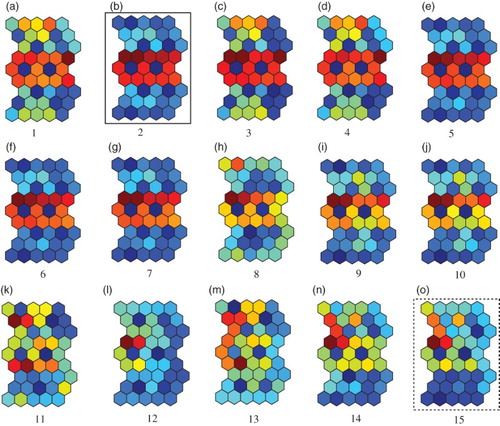
Figure 9 shows U-matrices when the parameter β was increased from one (a) to 15 (o). When the prediction performance was its highest and the parameter β was two in Figure 9(b), one of the most explicit U-matrices was obtained with a clearer class boundary in the middle of the map. In addition, when the prediction errors in MSE were relatively lower, for example, when the parameter β was five (e), six (f) and seven (g), clearer U-matrices were also obtained. However, when the prediction error was higher in Figure 9(o), we could not see any regularities in the U-matrix.

Figure 9. U-matrices with 5 by 3 neurons when the parameter β was increased from 1 (a) to 15 (o) with the best number of winners for the euro-yen exchange rates.

3.2.3. Interpretation

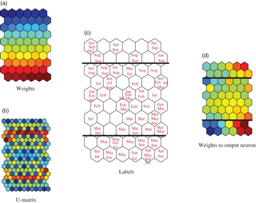
Figure 10 shows connection weights into competitive neurons (a), U-matrix (b), labels (c) and connection weights (d) into the output neuron for the best case in Figure 9 (b). As shown in the weights in Figure 10(a) and U-matrix in Figure 10(b), the weights and U-matrix were divided into upper and lower parts on the map. Labels in Figure 10(c) showed that the exchange rates in Figure 12 were divided into a higher part and lower part. The higher part was composed of ‘April’, ‘May’, and ‘June’, whereas the lower part was composed of ‘January’, ‘August’, ‘September’, and ‘October’. The boundary in the middle showed an intermediate part composed of ‘February’, ‘March’, and ‘July’. Figure 10(d) shows connection weights into the output neuron. Though connection weights did not show clearer characteristics, we could still see a separation between the lower and higher parts. Figure 11 shows connection weights into the competitive neurons (a), U-matrix (b), labels (c) and weights into the output neuron (d) when the prediction performance was the worst in Figure 9(o), though connection weights into the competitive neurons showed that they gradually became weaker from the upper side to the lower side of the map as shown in Figure 11(a). However, a class boundary in warm colours in Figure 11(b) was weaker than that obtained by contradiction resolution in Figure 10(b). The labels in Figure 11(c) were similar to those by contradiction resolution in Figure 10(c). The connection weights in Figure 11(d) seem to be separated into upper and lower parts by the class boundary.

Figure 10. U-matrix, labels, and weights from the first input neuron and weights into the output neuron when the parameter β was two and the number of winners was three for the euro-yen exchange rates.

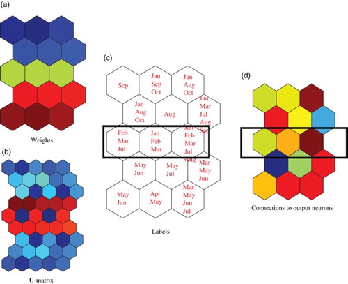
Figure 11. U-matrix, labels, and weights from the first input neuron and weights into the output neuron when the parameter β was 15 and the number of winners was three for the euro-yen exchange rates.

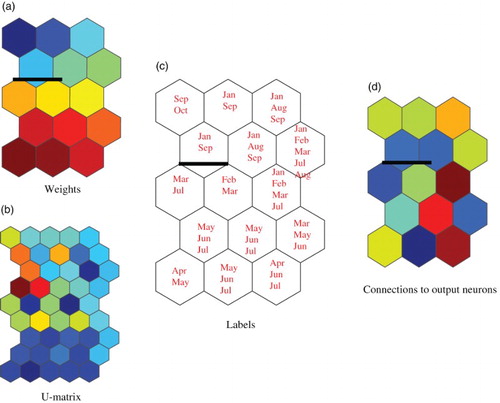
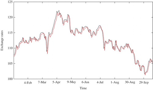
Figure 12. Euro-yen exchange rates during 2011.

3.2.4. Conventional methods

Table 5 shows the summary of results by the conventional SOM and two methods of the RBF network. By using the conventional SOM, the prediction error in the MSE was 0.546, which was much higher than the 0.436 by contradiction resolution in Table 4; however, a QE of 2.425 and TE of 0.172 were lower than those obtained by the contradiction resolution with the lowest prediction error. Nevertheless, the same level of QE and TEs could be obtained by our contradiction resolution, as in Table 4.

Table 5.  MSE for testing data, QEs, TEs and mutual information by the conventional SOM and RBF networks for the euro-yen exchange rates.

Size or methods	MSE	QE	TE	INF
SOM	0.546	2.425	0.172	1.258
FS	0.549
RR	0.507

Notes: The symbol ‘FS’ denotes the forward selection RBF with the generalisation cross validation and ‘RR’ denotes the Ridge regression RBF with the GCV.

Figure 13 shows weights to competitive neurons (a), U-matrix (b), labels (c) and connection weights into the output neuron (d) by the conventional SOM. Connection weights in Figure 13(a) showed clearly stronger lower parts and weaker upper parts on the connection weights. However, it was difficult to interpret a class boundary in Figure 13(b). In Figure 13(c), the labels showed the same tendency that months with higher rates were located on the lower side, while those with lower rates were located on the upper side. Months with intermediate rates were located between them. Connection weights into the output neuron showed the same tendency, that the higher values were located on the lower side, while lower values were on the higher side of the map in Figure 13 (d). We can say that the characteristics obtained by the conventional SOM were weaker than those by contradiction resolution, as seen in Figure 10.

Figure 13. U-matrix, labels, weights form the first input neuron and weights into the output neuron when the conventional SOM was used.

3.3. Euro-Yen exchange rate prediction: experiments with large size

3.3.1. Prediction performance

For the Euro-Yen exchange rates, we increased the network size from 5 by 3 to 10 by 6 neurons to examine whether better prediction performance could be obtained by an increase in map size. Table 6 shows the summary of experimental results with the 10 by 6 neurons for the Euro-Yen data. First, the number of winners was larger than that for the smaller size in Table 4. The largest number of winners was 40 when the parameter β was 40 and the smallest number of winners was 10 when the parameter β was 10. The lowest prediction error in the MSE was 0.441 when the parameter β was one. The MSE tended to increase slightly when the parameter β was increased. The QEs deceased from 3.036 for β=1 to 1.563 for β=15. The TEs decreased and then increased when the parameter β was increased. Mutual information increased when the parameter β was increased. The lower prediction errors did not corresponded to improved QEs, TEs and increased mutual information. In other words, the increase in organisation seemed to be contradictory to improved prediction performance.

Table 6.  The number of winners, MSE for testing data, QEs, TEs and mutual information when the parameter β was changed from one to 15 for the 10 by 6 maps for the Euro-yen exchange rates.

β	WIN	MSE	QE	TE	INF
1	40	0.441	3.036	0.292	1.081
2	40	0.443	3.012	0.313	1.085
3	31	0.447	2.698	0.115	1.146
4	24	0.449	2.524	0.208	1.220
5	21	0.442	1.995	0.130	1.297
6	27	0.447	2.265	0.089	1.235
7	13	0.453	1.786	0.141	1.343
8	20	0.475	1.882	0.104	1.311
9	20	0.453	1.831	0.104	1.320
10	10	0.463	1.642	0.161	1.371
11	25	0.464	1.942	0.057	1.293
12	12	0.457	1.879	0.125	1.346
13	16	0.466	1.628	0.182	1.363
14	21	0.458	1.669	0.156	1.350
15	16	0.464	1.563	0.172	1.373

Note: The number of winners (Win) was determined to minimise MSE.

3.3.2. Visual performance

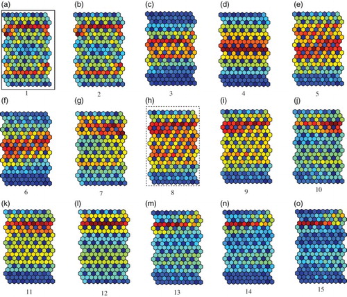
Figure 14 shows the U-matrices when the parameter β was increased from one (a) to 15 (o). When the parameter β was one in Figure 14(a), two class boundaries in warm colours were detected. Though QEs and TEs were larger and mutual information was smaller in Table 6, the U-matrix showed clear class boundaries. Two distinct class boundaries in Figure 14 gradually deteriorated when the parameter β was increased from three (c) to nine (i). Then, when the parameter β was 10 in Figure 14(j), one clear class boundary became explicit. When the parameter β was further increased, the class boundary became clearer. When the parameter β was 15 in Figure 14(o), the clearest boundary was detected. These results show that relatively clearer class boundaries were detected when the MSE was the lowest.

Figure 14. U-matrices with 10 by 6 neurons when the parameter β was increased from 1 (a) to 15 (o) with the best number of winners.

3.3.3. Interpretation

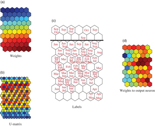
Figure 15 shows connection weights into competitive neurons (a), the U-matrix (b), labels (c) and connection weights into the output neuron (d) when the MSE was the lowest in Figure 6(a). Figure 15(a) shows connection weights into competitive neurons. The strength of connection weights gradually diminished from top to bottom. Figure 15(b) shows the U-matrix where two distinct class boundaries were detected. Figure 15(c) shows the labels, where we can see that months with lower rates (‘January’, ‘September’) were located on the upper side, while the months with higher rates (‘April’, ‘May’) were located on the lower side of the map in Figure 15. Months were rearranged according to the strength of the exchange rates. Figure 15 shows weights into the output neuron. In Figure 15(a), we could see that stronger weights were located on the upper and lower side of the map.

Figure 15. U-matrix, labels, weights from the first input neuron, weights into the output neuron when the parameter β was one and the number of winners was 40 for the euro-yen rates.

Figure 16 shows connection weights into the competitive neurons (a), U-matrix (c) and weights into the output neuron in Figure 16(d) when the MSE was the highest and the parameter β was eight. Though weights into the competitive neurons were the same as those for the best MSE case in Figure 15(a), the class boundaries became obscure in Figure 16(b), and the labels tended to gather at the centre of the map in Figure 16(c). In weights into the output neuron in Figure 16 (d), it was very hard to detect any regularity.

Figure 16. U-matrix, labels and weights from the first input neuron, weights into the output neuron when the parameter β was eight and the number of winners was 20.

3.3.4. Conventional methods

Table 7 shows the summary of experimental results by using the conventional SOM. The prediction error in MSE was 0.522 in Table 7, which was larger than any prediction errors in MSE by contradiction resolution in Table 6. The QE of 1.271 was lower than any values by contradiction resolution in Table 6. The TE of 0.297 was fairly larger than those by contradiction resolution in Table 6. The mutual information of 1.410 was larger than any values by contradiction resolution in Table 6. The lower prediction error in MSE was obtained by sacrificing QEs and mutual information, and TEs. Figure 17 shows labels, weights and U-matrix by the conventional SOM. We could not see any regularities in the U-matrix in Figure 17(b). In addition, weights to the output neuron showed almost random patterns.

Figure 17. U-matrix, labels, weights form the first input neuron and weights into the output neuron when the conventional SOM was used for the euro-yen data.

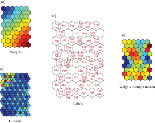
Table 7.  MSE for testing data, QEs, TEs and mutual information by the conventional SOM for the euro-yen exchange rates.

Size or methods	MSE	QE	TE	INF
SOM	0.522	1.271	0.297	1.410

3.4. Discussion

3.4.1. Validity of methods and experimental results

The implication of the experimental results can be explained by three points, namely, a new interpretation method for SOM, multiple winners and neural networks in general. First, our method can be used, as discussed in the introduction section, to interpret SOM knowledge. The SOM (Kohonen, 1988; Kohonen, 1995) has been a popular method to visualise complex data with a number of applications. However, the main problem of SOM lies in its difficulty in interpreting final knowledge of the SOM. When it is applied to class structure detection, class boundaries are ambiguous and hard to interpret. Thus, many computational methods have been proposed to clarify the final knowledge obtained by the SOM (Kaski et al., 1998; Mao & Jain, 1995; Merényi et al., 2009; Tasdemir & Merényi, 2009; Ultsch & Siemon, 1990; Vesanto, 1999). However, with any kinds of computational methods, it is still hard to interpret the final representations. The contradiction resolution used in the present paper showed clearer class structure in both data sets. This shows that the method can be used to provide more easily interpretable knowledge for the SOM.

Second, the importance of neurons in the present method can be discussed in the framework of multiple winners in neural networks. Neural networks are called ‘winner-take-all’ when they try to take the most prominent response to the input pattern. The winner-take-all operations have been extensively used in neural networks with many applications. One of the extensions of the winner-take-all network is KWTA or k-winner-take-all, which takes the k largest elements instead of one element. The KWTA has proved to be a powerful network (Maass, 2000) with improved performance in many applications (Ridella et al., 2001; Urahama & Nagao, 1995; Wolfe et al., 1991).

In addition, in cognitive computing, multi-winners-take all has been highly plausible as a model of the actual neural mechanisms of living systems (Gros, 2009; O'Reilly, 1998). In the multi-winners-take-all operations, the winning coalition of neurons tends to suppress the activities of all other ones. The coalitions of neurons together were considered as the essential building blocks of the human mind (Crick & Koch, 2003; Koch, 2004).

Third, our method is related to attempts to interpret internal representations created by neural networks. One of the main objectives of neural networks is to interpret final representations. This objective has been explored from the beginning of the birth of conventional neural computation (Feraud & Clerot, 2002; Howes & Crook, 1999; Ishikawa, 1996; Ishikawa, 2000; Micheli et al., 2001; Nord & Jacobsson, 1998; Rumelhart et al., 1986; Setiono et al., 2002; Towell & Shavlik, 1993), to cite a few. However, connection weights obtained by neural networks are extremely complex, which has prevented us from interpreting the final representations. Our method is used to visualise input patterns over a fixed lattice following the SOMs. Thus, the method is a new method to interpret final representations in neural networks in general.

3.4.2. Limitation of the method

Though improved performance in terms of prediction and visualisation was obtained, two problems should be pointed out, namely, the optimal values of the parameter β with the appropriate number of winners, and relations to QEs and TEs.

Though we succeeded in showing the possibility of improved prediction performance by adjusting the number of winning neurons and the parameter β, we could not show how to obtain optimal values for the number of winning neurons and the parameter β. To obtain the optimal values of the parameter β and the number of winners, we must exhaustively search for the optimal values. The main problem is that there are no explicit criteria to measure the interpretability of final representations. We tried to use mutual information as a measure of organisation in Tables 123456–7. However, we noticed that higher mutual information was not accompanied by improved visualisation in Figures 4, 9 and 14. Thus, we need to develop a method of measuring the interpretability of representations and to relate it to prediction performance as well as to adjust the number of winners and the parameter β.

Second, smaller prediction errors were not necessarily accompanied by smaller QEs and TEs, as in Tables 1, 4, 6 and Figures 4, 9, 14. Though connection weights by our method were visually and easily interpreted, careful attention should be paid to the interpretation of connection weights, because the weights may not reflect the characteristics of input patterns in terms of QEs and QEs. We think that we need to develop a method at least to relate visualisation and prediction to QEs and TEs. Ideally, we should develop a method to quantify the degree of interpretation as mentioned above.

3.4.3. Possibility of the method

We can point out two directions of our method, namely, close relations between interpretation and prediction and extension to different types of evaluation.

First, our method opens up the possibility of examining relations between improved interpretation and better prediction performance. In neural networks, one of the main problems is that it is hard to interpret internal representations obtained by learning in neural networks with better prediction performance. Improved prediction and interpretation performance have been independently pursued, often independent of one another. The present experimental results have shown that visualisation or interpretation in competitive learning is directly related to improved prediction performance. If prediction is correlated with interpretation, we can explore the improved performance of neural networks in a unified way or in terms of prediction and interpretation at the same time. For example, we can explore how some improvement in interpretation affects prediction performance.

Second, we have the possibility that two types of evaluation can be extended to multiple types of evaluation. We limited ourselves to two types of evaluation in the present paper. However, we can imagine many different kinds of evaluation. For example, we can consider mutual interaction between different types of neurons. If two types of evaluation interact with each other, then the evaluation used should be mutual evaluation. If it is possible to take into account many different kinds of evaluation, our method can be more easily generalised and applied to many practical problems.

4. Conclusion

In this paper, we proposed a new type of information-theoretic method called ‘contradiction resolution’. We improved contradiction resolution in two ways. First, self-evaluation and outer-evaluation were clearly separated. We were able to more clearly see the difference or contradiction between self and outer-evaluation using this separation. In addition, the importance of neurons was taken into account in each evaluation. In considering the importance of neurons, each neuron was evaluated by the limited number of important neurons. According to the ranking of neurons, we could use the appropriate number of neurons for evaluation. We applied the method to two data sets, namely, the Senate and Euro-yen exchange rates. In both data sets, we could see that prediction performance was improved by changing the number of winners. Final connection weights were easily interpreted intuitively. In addition, we saw that visualisation performance was proportional to prediction performance.

Though there are some problems such as parameter tuning and topological preservation, our method shows that it is possible to view neurons from different points of view, and that the contradiction between those views should be reduced as much as possible.

Appendix

Minimising KL-divergence

We here present how to obtain the optimal firing rates of the jth neuron for the sth input pattern p*(j | s) (Kunisawa, 1975). Supposing that the probability p(j | s) for neurons by the self-evaluation and q(j | s) denotes the firing probability of neurons by the outer-evaluation, which is supposed to be fixed. then we must decrease the following KL divergence measure for each input pattern:

In minimising the KL divergence, we suppose that the corresponding cost E^s of assigning input patterns to competitive units is represented by QEs between input patterns and connection weights:

where

When this QE is fixed, the optimal probability p*(j | s) to minimise the KL divergence is obtained by

Now, using the parameters λ and μ, we have

Then, transforming the above equation, we have

where

To minimise U, we must minimise the first term

Because this term is always greater than zero or equal to zero, minimum optimal probability is obtained by

Now, substituting μ by 1/2σ², we have the equation used in the main text.

References

- Bauer, H.-U., & Pawelzik, K. (1992). Quantifying the neighborhood preservation of self-organizing maps. IEEE Transactions on Neural Networks, 3(4), 570–578. doi: 10.1109/72.143371
- Chen, S., Cowan, C., & Grant, P. (1991). Orthogonal least squares learning algorithm for radial basis function networks. IEEE Transactions on Neural Networks, 2(2), 302–309. doi: 10.1109/72.80341
- Crick, F., & Koch, C. (2003). A framework for consciousness. Nature Neuroscience, 6(2), 119–126. doi: 10.1038/nn0203-119
- De Runz, C., Desjardin, E., & Herbin, M. (2012). Unsupervised visual data mining using self-organizing maps and a data-driven color mapping. 16th international conference on Information Visualisation (IV), 2012, Montpellier, IEEE, 241–245.
- DeSieno, D. (1988). Adding a conscience to competitive learning. Proceedings of IEEE international conference on neural networks, San Diego, IEEE, 117–124.
- Feraud, R., & Clerot, F. (2002). A methodology to explain neural network classification. Neural Networks, 15, 237–246. doi: 10.1016/S0893-6080(01)00127-7
- Golub, G., Heath, M., & Wahba, G. (1979). Generalized cross-validation as a method for choosing a good ridge parameter. Technometrics, 21(2), 215–223. doi: 10.1080/00401706.1979.10489751
- Gros, C. (2009). Cognitive computation with autonomously active neural networks: An emerging field. Cognitive Computation, 1(1), 77–90. doi: 10.1007/s12559-008-9000-9
- Howes, P., & Crook, N. (1999). Using input parameter influences to support the decisions of feedforward neural networks. Neurocomputing, 24, 191–206. doi: 10.1016/S0925-2312(98)00102-7
- Ishikawa, M. (1996). Structural learning with forgetting. Neural Networks, 9(3), 509–521. doi: 10.1016/0893-6080(96)83696-3
- Ishikawa, M. (2000). Rule extraction by successive regularization. Neural Networks, 13, 1171–1183. doi: 10.1016/S0893-6080(00)00072-1
- Kamimura, R. (2012a). Contradiction resolution and its application to self-organizing maps. The 2012 international joint conference on SMC, Seoul, IEEE.
- Kamimura, R. (2012b). Controlling relations between the individuality and collectivity of neurons and its application to self-organizing maps. Neural Processing Letters, 38, 1–27.
- Kamimura, R. (2012c). Interaction of individually and collectively treated neurons for explicit class structure in selforganizing maps. The 2012 international joint conference on Neural networks (IJCNN), Brisbane, IEEE, 1–8.
- Kaski, S., Nikkila, J., & Kohonen, T. (1998). Methods for interpreting a self-organized map in data analysis. Proceedings of European symposium on artificial neural networks, Bruges, Belgium.
- Kaski, S., Nikkila, J., Oja, M., Venna, J., Toronen, P., & Castren, E. (2003). Trustworthiness and metrics in visualizing similarity of gene expression. BMC Bioinformatics, 4(48).
- Kiviluoto, K. (1996). Topology preservation in self-organizing maps. Proceedings of the IEEE international conference on neural networks, Washington, DC, 294–299.
- Koch, C. (2004). The quest for consciousness: A neurobiological approach. Englewood, CO: Robert & Company Publishers.
- Kohonen, T. (1988). Self-organization and associative memory. New York, NY: Springer-Verlag.
- Kohonen, T. (1990). The self-organizing maps. Proceedings of the IEEE, 78(9), 1464–1480. doi: 10.1109/5.58325
- Kohonen, T. (1995). Self-organizing maps. Berlin: Springer-Verlag.
- Kunisawa, K. (1975). Entropy model (in Japanese). Tokyo: Nikkagiren.
- Lee, J. A., and Verleysen, M. (2008). Quality assessment of nonlinear dimensionality reduction based on K-ary neighborhoods. JMLR: Workshop and conference proceedings, Antwerp, Vol. 4, 21–35.
- Maass, W. (2000). On the computational power of winner-take-all. Neural Computation, 12(11), 2519–2535. doi: 10.1162/089976600300014827
- Mao, I., & Jain, A. K. (1995). Artificial neural networks for feature extraction and multivariate data projection. IEEE Transactions on Neural Networks, 6(2), 296–317. doi: 10.1109/72.363467
- Merenyi, E., & Jain, A. (2004). Forbidden magnification? II. Proceedings of 12th European symposium on artificial neural networks, Bruges, Belgium, 57–62.
- Merenyi, E., Jain, A., & Villmann, T. (2007). Explicit magnification control of self-organizing maps for forbidden data. IEEE Transactions on Neural Networks, 18(3), 786–797. doi: 10.1109/TNN.2007.895833
- Merényi, E., Tasdemir, K., & Zhang, L. (2009). Learning highly structured manifolds: Harnessing the power of soms. In Similarity-based clustering (pp. 138–168). Berlin: Springer.
- Micheli, A., Sperduti, A., & Starita, A. (2001). Analysis of the internal representations developed by neural networks for structures applied to quantitative structure-activity relationship studies of benzodiazepines. Journal of Chemical Information and Computer Sciences, 41, 202–218.
- Nord, L. I., & Jacobsson, S. P. (1998). A novel method for examination of the variable contribution to computational neural network models. Chemometrics and Intelligent Laboratory Systems, 44, 153–160. doi: 10.1016/S0169-7439(98)00118-X
- O'Reilly, R. (1998). Six principles for biologically based computational models of cortical cognition. Trends in Cognitive Sciences, 2(11), 455–462. doi: 10.1016/S1364-6613(98)01241-8
- Orr, M. (1996). Introduction to radial basis function networks (Technical report). Center for cognitive science, University of Edinburgh.
- Orr, M. (1999). Matlab functions for radial basis function networks. Institute for Adaptive and Neural Computation, Division of Informatics, Edinburgh University, Edingburgh EH8 9LW.
- Polzlbauer, G. (2004). Survey and comparison of quality measures for self-organizing maps. Proceedings of the fifth workshop on data analysis (WDA04), Slovakia, 67–82.
- Ridella, S., Rovetta, S., & Zunino, R. (2001). K-winner machines for pattern classification. IEEE Transactions on Neural Networks, 12(2), 371–385. doi: 10.1109/72.914531
- Romesburg, H. C. (1984). Cluster analysis for researchers. Belmont, CA: Life time learning publishers.
- Rumelhart, D. E., Hinton, G. E., & Williams, R. (1986). Learning internal representations by error progagation. In D. E. Rumelhart et al. (Eds.), Parallel distributed processing (Vol. 1, pp. 318–362). Cambridge: MIT Press.
- Setiono, R., Leow, W. K., & Zurada, J. M. (2002). Extracting of rules from artificial neural networks for nonlinear regression. IEEE Transactions on Neural Networks, 13(3), 564–577. doi: 10.1109/TNN.2002.1000125
- Shieh, S., & Liao, I. (2012). A new approach for data clustering and visualization using self-organizing maps. Expert Systems with Applications, 5, 11924–11933. doi: 10.1016/j.eswa.2012.02.181
- Su, M.-C., & Chang, H.-T. (2001). A new model of self-organizing neural networks and its application in data projection. IEEE Transactions on Neural Networks, 123(1), 153–158.
- Tasdemir, K., & Merényi, E. (2009). Exploiting data topology in visualization and clustering of self-organizing maps. IEEE Transactions on Neural Networks, 20(4), 549–562. doi: 10.1109/TNN.2008.2005409
- Towell, G. G., & Shavlik, J. W. (1993). Extracting refined rules from knowledge-based neural networks. Machine Learning, 13, 71–101.
- Ultsch, A., & Siemon, H. P. (1990). Kohonen self-organization feature maps for exploratory data analysis. In Proceedings of international neural network conference (pp. 305–308). Dordrecht: Kulwer Academic Publisher.
- Urahama, K., & Nagao, T. (1995). K-winners-take-all circuit with o (n) complexity. IEEE Transactions on Neural Networks, 6(3), 776–778. doi: 10.1109/72.377986
- Van Hulle, M. (1996). Topographic map formation by maximizing unconditional entropy: A plausible strategy for ‘on-line’ unsupervised competitive learning and nonparametric density estimation. IEEE Transactions on Neural Networks, 7(5), 1299–1305. doi: 10.1109/72.536323
- Van Hulle, M. M. (1997). The formation of topographic maps that maximize the average mutual information of the output responses to noiseless input signals. Neural Computation, 9(3), 595–606. doi: 10.1162/neco.1997.9.3.595
- Van Hulle, M. M. (1999). Faithful representations with topographic maps. Neural Networks, 12(6), 803–823. doi: 10.1016/S0893-6080(99)00041-6
- Van Hulle, M. M. (2004). Entropy-based kernel modeling for topographic map formation. IEEE Transactions on Neural Networks, 15(4), 850–858. doi: 10.1109/TNN.2004.828763
- Venna, J., & Kaski, S. (2001). Neighborhood preservation in nonlinear projection methods: An experimental study. In G. Dorffner, H. Bischof, & Kurt Hornik (Eds.), Lecture notes in computer science (Vol. 2130, pp. 485–491). Berlin: Springer.
- Vesanto, J. (1999). SOM-based data visualization methods. Intelligent Data Analysis, 3, 111–126. doi: 10.1016/S1088-467X(99)00013-X
- Vesanto, J., Himberg, J., Alhoniemi, E., & Parhankangas, J. (2000a). SOM toolbox for Matlab (Technical report). Laboratory of Computer and Information Science, Helsinki University of Technology.
- Vesanto, J., Himberg, J., Alhoniemi, E., & Parhankangas, J. (2000b). SOM toolbox for matlab 5 (Technical Report A57). Helsinki University of Technology.
- Villmann, T., & Claussen, J. C. (2006). Magnification control in self-organizing maps and neural gas. Neural Computation, 18, 446–469. doi: 10.1162/089976606775093918
- Villmann, T., Herrmann, R. D. M., & Martinez, T. (1997). Topology preservation in self-organizing feature maps: Exact definition and measurment. IEEE Transactions on Neural Networks, 8(2), 256–266. doi: 10.1109/72.557663
- Wolfe, W., Mathis, D., Anderson, C., Rothman, J., Gottler, M., Brady, … Alaghband, G. (1991). K-winner networks. IEEE Transactions on Neural Networks, 2(2), 310–315. doi: 10.1109/72.80342
- Wu, S., & Chow, T. (2005). Prsom: A new visualization method by hybridizing multidimensional scaling and self-organizing map. IEEE Transactions on Neural Networks, 16(6), 1362–1380. doi: 10.1109/TNN.2005.853574
- Xu, L., & Chow, T. (2011). Multivariate data classification using polsom. Prognostics and system health management conference (PHM-Shenzhen), 2011, Shenzhen, IEEE, 1–4.
- Xu, L., Xu, Y., & Chow, T. W. (2010). PolSOM-a new method for multidimentional data visualization. Pattern Recognition, 43, 1668–1675. doi: 10.1016/j.patcog.2009.09.025
- Xu, Y., Xu, L., & Chow, T. (2011). Pposom: A new variant of polsom by using probabilistic assignment for multidimensional data visualization. Neurocomputing, 74(11), 2018–2027. doi: 10.1016/j.neucom.2010.06.028
- Yin, H. (2002). ViSOM-a novel method for multivariate data projection and structure visualization. IEEE Transactions on Neural Networks, 13(1), 237–243. doi: 10.1109/72.977314
- Zhang, L., Merényi, E., Grundy, W. M., & Young, E. F. (2010). Inference of surface parameters from near-infrared spectra of crystalline ice with neural learning. Publications of the Astronomical Society of the Pacific, 122(893), 839–852. doi: 10.1086/655115