Modeling development of natural multi-sensory integration using neural self-organisation and probabilistic population codes

Abstract

Humans and other animals have been shown to perform near-optimally in multi-sensory integration tasks. Probabilistic population codes (PPCs) have been proposed as a mechanism by which optimal integration can be accomplished. Previous approaches have focussed on how neural networks might produce PPCs from sensory input or perform calculations using them, like combining multiple PPCs. Less attention has been given to the question of how the necessary organisation of neurons can arise and how the required knowledge about the input statistics can be learned. In this paper, we propose a model of learning multi-sensory integration based on an unsupervised learning algorithm in which an artificial neural network learns the noise characteristics of each of its sources of input. Our algorithm borrows from the self-organising map the ability to learn latent-variable models of the input and extends it to learning to produce a PPC approximating a probability density function over the latent variable behind its (noisy) input. The neurons in our network are only required to perform simple calculations and we make few assumptions about input noise properties and tuning functions. We report on a neurorobotic experiment in which we apply our algorithm to multi-sensory integration in a humanoid robot to demonstrate its effectiveness and compare it to human multi-sensory integration on the behavioural level. We also show in simulations that our algorithm performs near-optimally under certain plausible conditions, and that it reproduces important aspects of natural multi-sensory integration on the neural level.

Keywords:

• multi-sensory integration
• brain modeling
• self-organisation
• probabilistic population codes
• superior colliculus

1. Introduction

^†Integration of input to different sensory modalities presents an organism with complementary information about its environment. Natural organisms have therefore developed various independent sensory organs and ways to integrate their input (Stein & Meredith, 1993). Among the benefits of integrating signals from different modalities are shorter reaction times, greater perceptual accuracy, and lower thresholds of stimulus detection (Ernst & Banks, 2002; Frassinetti et al., 2002; Gori et al., 2008; Neil et al., 2006).

Uncertainty in sensory information makes tasks in sensory processing and especially in multi-sensory integration exercises in probabilistic inference. Humans and other animals have been shown to perform near-optimally in such tasks in the sense that they integrate information from different sources taking into account its uncertainty (Alais & Burr, 2004; Ernst & Banks, 2002; Gori, Sandini, & Burr, 2012; Landy, Banks, & Knill, 2011). Since natural sensory processing produces results compatible with optimal probabilistic inference, representations of probabilistic information have been looked for in neurons performing sensory processing, and found (Yang & Shadlen, 2007).

An explanation of how neural hardware can produce such representations and perform probabilistic reasoning on them is necessary to understand natural multi-sensory integration. It is especially important to understand how neurons or networks of neurons can acquire the knowledge about the statistics of the organism's environment that is the basis of these computations. Xu, Yu, Rowland, Stanford, and Stein (2012) have shown that cats can learn audio–visual integration even if they are raised in an environment in which none of the audio–visual stimuli they perceive has any behavioural relevance, that is, they do not herald food or signal any other change in the environment which the animals can perceive. This suggests that learning is at least partially unsupervised (Xu et al., 2012). Finally, a model of biological multi-sensory integration on the neural level which explains probabilistic reasoning and acquisition of the requisite statistical knowledge also needs to exhibit the known neurophysiology.

Topographic mapping is a pervasive principle in sensory processing (Imai, Sakano, & Vosshall, 2010; Kaas, 1997; King, 2013; Stein & Stanford, 2008; Yang & Shadlen, 2007). In topographic mapping, a sensory variable L is represented by the joint activity of a whole population of neurons; that is, in a population code (Georgopoulos, Schwartz, & Kettner, 1986; Seung & Sompolinsky, 1993): each neuron in the population has a preferred value l of L and responds strongest to that value l. The topology of preferred values in the population reflects that of the sensory variable; neurons which are close to each other have similar preferred values and the location of the peak activity in the population corresponds to the value l of L being encoded.

Of particular interest are probabilistic population code (PPCs), and especially topographic PPCs, population codes in which each neuron has a preferred value of some variable and encodes in its activity the probability of this value given the input (Pouget, Dayan, & Zemel, 2003). Such codes can be said to encode probability density function (PDFs) over sensory variables and they are one possible component of probabilistic processing in neural networks.

Recent studies have proposed artificial neural network (ANN) models which carry out computations on PPCs, like performing Bayesian inference (Beck et al., 2008; Cuijpers & Erlhagen, 2008; Fetsch, DeAngelis, & Angelaki, 2013). The algorithms proposed in their studies combine PPCs, and do not consider the problem of computing PPCs from sensory input. In contrast, Barber, Clark, and Anderson (2003) and Jazayeri and Movshon (2006) proposed ANN models which can compute PPCs from sensory input. Yet these models are not adaptive and knowledge of tuning functions and noise properties of the input neurons needs to be encoded into the configuration of the networks.

Soltani and Wang (2010) presented a model of reward-based neural learning and probabilistic decision-making which reproduces firing patterns of biological neurons found in the lateral intraparietal area of monkeys in a weather prediction task (Yang & Shadlen, 2007). For all its explanatory power, Soltani and Wang’s (2010) model does not learn unsupervised, it does not account for inference on continuous input, as opposed to categorical input, and it does not reproduce topographic mapping.

Zhou, Dudek, and Shi (2011) and Bauer, Weber, and Wermter (2012) have proposed ANN algorithms based on the self-organising map (SOM), which can learn tuning functions and noise properties of sensory input neurons. After learning, the SOM units in Zhou et al.’s, (2011) and Bauer, Weber et al.’s, (2012) networks each compute a probability for a given value of the sensory variable being encoded. Typically, when we map a data point into a trained SOM, we are not interested in the full population response. Instead, we reduce that population response to the index of just one best-matching unit (BMU), emulating winner-take-all-like network dynamics in biological neuron populations. The whole population response can be of interest in SOM variants whose neurons each compute the probability of one possible cause of their input: as Zhou et al. (2011) pointed out, these SOM variants generate PPCs encoding PDF over the latent variables of the data. Both networks, that of Zhou et al. (2011) and Bauer, Weber et al. (2012), however, assume Gaussian noise in their input, limiting their flexibility and biological plausibility.

In this paper, we propose a model of learning and performing optimal multi-sensory integration. The model is based on a self-organising ANN algorithm we recently proposed (Bauer & Wermter, 2013). The network in this algorithm learns the tuning functions and noise properties of its input neurons and self-organises to compute a PPC encoding a PDF over values of a sensory variable. We make very light assumptions on tuning functions and noise properties in input neurons, and computations are simple. Our network is quite general in principle. Nevertheless, it is based on and strives to model known biology of the superior colliculus (SC). The SC is a well-studied region in the vertebrate mid-brain which integrates input from multiple sensory modalities to localise stimuli in space (King, 2013). Here, we will show that our network reproduces important aspects of SC biology and psychophysics of multi-sensory object localisation. For the purposes of modeling natural multi-sensory integration, we slightly simplify this algorithm on the one hand, and extend it with divisive normalisation on the other (Fetch et al., 2013).

In Section 2, we will first mathematically formulate the problem of computing a PPC for the position of a stimulus from noisy sensory input. We will then introduce a network structure and computations to carry out this task, and an algorithm for training it. To validate our model, we show in Section 3 that the algorithm can be used effectively in a real-world scenario by testing it in a robotic audio–visual object localisation task and demonstrate that audio–visual integration in our model is similar to the near-optimal integration found in a human experiment by Alais and Burr (2004). In Section 4, we use simulations to show that our network not only integrates localisations from different modalities, but actually uses all available information efficiently, regardless of origin. These simulations also allow us to choose parameters to make detailed simulated neural response properties of our network observable which are similar to those found in the SC.

2. Probabilistic population codes and learning to compute them

The problem faced by the SC is well described as a statistical inference problem: let $\mathbf{\text{I}}={\mathbf{\text{i}}}_1,{\mathbf{\text{i}}}_2,\dots ,{\mathbf{\text{i}}}_{n_i}$ be all the neurons projecting to the SC and $\mathbf{\text{A}}={\mathbf{\text{a}}}_1,{\mathbf{\text{a}}}_2,\dots ,{\mathbf{\text{a}}}_{n_i}$ be their activity, with n_i being the total number of input neurons. Assuming that this activity is driven by the presence of some cross-sensory stimulus, it is the task of the SC to determine the location L of the stimulus. Since responses of biological neurons are variable between presentations of the same stimulus, localisation will have some uncertainty. This uncertainty is expressed in the probability distribution $P(\mathrm{L}|\mathbf{\text{A}})$ over the possible values of the random variable L given input activity A. That probability distribution is given by Bayes’ theorem: (1) $P(L|\mathbf{\text{A}})=\frac{P(\mathbf{\text{A}}|L)}{P(\mathbf{\text{A}})}P(L),$(1) where P(L) is the prior probability distribution for L.

In a PPC, every output neuron o in the population of output neurons $\mathbf{\text{O}}={\mathbf{\text{o}}}_1,{\mathbf{\text{o}}}_2,\dots ,{\mathbf{\text{o}}}_{n_o}$ encodes in its activity the probability of one value of the sensory variable being encoded – in this case, the probability of one location $l_{\mathbf{\text{o}}}$ being the true location L of the stimulus. If we assume that the SC's output is a PPC, then the activity of every output neuron o will have to follow Equation (1), substituting o’s preferred value $l_{\mathbf{\text{o}}}$ for L.

At this level of generality, implementing the computations necessary to produce a PPC in a neural network presents a number of problems. The statistical relationship between the latent variable L and the population response A could have arbitrary complexity going well beyond the computational capabilities of an individual neuron or a small sub-population. Also, whatever statistical relationship there is between L and A, it will depend on the phenotype of the organism and its specific environment. It is therefore not plausible that this relationship is fully encoded genetically; it will have to be at least partially learned. In the following, we will explain which reasonable simplifications we can make and how the knowledge which is necessary to infer object location from noisy sensory input can be acquired.

2.1. Network structure and computations

We will start by explaining the network architecture and the computations realised in it, which implement the above considerations once the network is trained, leaving the actual training mechanism to the next section.

As noted above, the relationship between the position of the stimulus L and the population response A could be of arbitrary complexity in principle. We will make the assumption, however, that the components of A, that is, individual input neurons’ activities, are statistically independent given L. This is to say we assume uncorrelated noise in the input neurons’ responses.

Uncorrelated noise makes the computations which an output neuron o has to carry out much simpler. Equation (1) becomes $P(L|\mathbf{\text{A}})=\frac{\prod _{k=1}^{n_i}P({\mathbf{\text{a}}}_k|L)}{P(\mathbf{\text{A}})}P(L).$ Assuming that L is uniformly distributed, we can drop the prior. Also, since P(A) is independent of L, we can ignore it for now; we will come back to it later. With this simplification, each of our neurons o will only have to compute the likelihood of the input for its preferred value $l_{\mathbf{\text{o}}}$: (2) $p(l_{\mathbf{\text{o}}}|\mathbf{\text{A}})\sim \prod _{k=1}^{n_i}p({\mathbf{\text{a}}}_k|l_{\mathbf{\text{o}}})$(2)

We have not made any assumptions about the tuning functions of the input neurons and the noise in their responses so far, except that we assumed that noise between neurons is uncorrelated and, implicitly, that the response of the neurons is statistically dependent of L. The probability $p({\mathbf{\text{a}}}_k|l_{\mathbf{\text{o}}})$ could therefore be proportional to an arbitrary function of the input $f({\mathbf{\text{a}}}_k)$. Rather than making additional strong assumptions on f or letting our neurons perform complex functions which are not likely to be computable by real neurons or simple neural sub-populations, we let each of our model neurons maintain one histogram of input activities for each of its input neurons (Figure 1).

Figure 1. Network architecture. Left: single output neuron. Right: network connectivity, flow of activation.

For our purposes, a histogram is represented by a list of counts of occurrences, one for each of the histogram's n_b bins. Let o be an output neuron with preferred value $l_{\mathbf{\text{o}}}$ of L and i be an input neuron connected to o. Then, we denote with $c_{\mathbf{\text{o}},\mathbf{\text{i}},b}$ the bth entry of the histogram kept by o to keep track of past input activities from i whenever L was $l_{\mathbf{\text{o}}}$. Let us assume that learning has taken place and made sure that the histograms are sufficiently representative of the input statistics in the sense just stated. Then, the probability density of input neuron i having activity ${\mathbf{\text{a}}}_{\mathbf{\text{i}}}$ given that L has value l_o can be approximated using the histogram: $p({\mathbf{\text{a}}}_{\mathbf{\text{i}}}|l_{\mathbf{\text{o}}})\approx \frac{c_{\mathbf{\text{o}},\mathbf{\text{i}},\lfloor {\mathbf{\text{a}}}_{\mathbf{\text{i}}}\rfloor }}{\sum _{b=1}^{n_b}{c}_{\mathbf{\text{o}},\mathbf{\text{i}},b}},$ where the activity ${\mathbf{\text{a}}}_{\mathbf{\text{i}}}$ rounded off to the nearest integer is used as a bin index.

Let the initial activity ${\widehat{\mathbf{\text{a}}}}_{\mathbf{\text{o}}}$ of an output neuron o in response to the input activity $\mathbf{\text{A}}={\mathbf{\text{a}}}_{\mathbf{\text{i}},1},{\mathbf{\text{a}}}_{\mathbf{\text{i}},2},\dots ,{\mathbf{\text{a}}}_{\mathbf{\text{i}},n_i}$ be ${\widehat{\mathbf{\text{a}}}}_{\mathbf{\text{o}}}=\prod _{k=1}^{n_i}\frac{c_{\mathbf{\text{o}},{\mathbf{\text{i}}}_k,\lfloor {\mathbf{\text{a}}}_{\mathbf{\text{i}},k}\rfloor }}{\sum _{b=1}^{n_b}{c}_{\mathbf{\text{o}},{\mathbf{\text{i}}}_k,b}}.$ Then that initial response would approximate the likelihood $p(\mathbf{\text{A}}|{\mathrm{l}}_{\mathbf{\text{o}}})$ of the input given that the actual value of the input stimulus L is o’s preferred value $l_{\mathbf{\text{o}}}$. The initial population response is then proportional to a PDF over L.

The actual gain of the population response would have great variability, however, because we dropped the normalisation factor $1/P(\mathbf{\text{A}})$ in Equation (2); as the likelihood of the input as a whole changes, so does the gain of the unnormalised likelihood function. The normalisation factor is not needed to compute relative probabilities for different values l of L or find the most probable value l, as $1/P(\mathbf{\text{A}})$ is independent of l. Real neurons only have a limited dynamic range, though. We therefore keep neural activity within a certain range by having our network perform divisive normalisation as suggested by Fetsch et al. (2013). The final activity ${\mathbf{\text{a}}}_{{\mathbf{\text{o}}}_m}$ of each output neuron ${\mathbf{\text{o}}}_m\in \mathbf{\text{O}}$ is therefore computed as ${\mathbf{\text{a}}}_{{\mathbf{\text{o}}}_m}=\frac{{\widehat{\mathbf{\text{a}}}}_{{\mathbf{\text{o}}}_m}}{(1/n_o)\sum _{k=1}^{n_o}{\widehat{\mathbf{\text{a}}}}_{{\mathbf{\text{o}}}_k}}.$

2.2. Learning histograms and dividing responsibilities

Next, we will describe the learning algorithm which will initialise the histograms to make the calculations possible which have been laid out thus far. Suppose that an output neuron o has a preferred value l. A supervised learning algorithm could update o’s histograms relatively easily: whenever the true position L of the stimulus is l, the algorithm could increase the value of that bin in each of o’s histograms corresponding to the current input (3) $c_{\mathbf{\text{o}},\mathbf{\text{i}},\lfloor {\mathbf{\text{a}}}_{\mathbf{\text{i}}}\rfloor }\leftarrow c_{\mathbf{\text{o}},\mathbf{\text{i}},\lfloor {\mathbf{\text{a}}}_{\mathbf{\text{i}}}\rfloor }+1,$(3) for each input neuron i with activity ${\mathbf{\text{a}}}_{\mathbf{\text{i}}}$.

Unfortunately, the true position L of the stimulus is usually not known to the model SC – inferring it from the input is precisely the task it needs to learn. Also, a neuron only has a preferred value once it responds strongest to some stimulus. Without prior knowledge about input statistics, any preference of one stimulus value over another will be weak and coincidental and not follow any topographic organisation in the network. Therefore, what we want our algorithm to do is (1) imprint a topographic map on our network such that neighbouring neurons have similar preferred values and (2) update the histograms of each of our neurons to reflect the statistics of the input (with 1 and 2 being mutually dependent).

One unsupervised learning algorithm which is able to train a network of neurons (or ‘units’) such that it develops a spatial organisation as described above is the SOM algorithm (Kohonen, 1982). A SOM is an abstract ANN, in which each neuron has a weight vector and computes as its response to some input vector of the same length the Euclidean distance of that weight vector from the input. That neuron with the least response to some input (the one whose weight vector is closest to the input) is called the ‘winner neuron’ or BMU. In every step of the learning algorithm, it presents the network with some input and updates the BMU together with its neighbourhood, moving their weight vectors a bit closer to the input vector in the Euclidean space. The strength of the update to each neuron decreases with increasing distance from the BMU.

The basic idea of this algorithm can be used to accomplish both goals (1) and (2): the supervised learning rule stated in Equation (3) updates that neuron whose preferred value of the input stimulus is the actual value of the input stimulus. In contrast, our new unsupervised algorithm selects that neuron ${\mathbf{\text{o}}}_B$ with the strongest response to the input (which we will also call the BMU) and then updates all neurons o, with the update strength depending on the distance between ${\mathbf{\text{o}}}_B$ and o in the network $c_{\mathbf{\text{o}},\mathbf{\text{i}},\lfloor {\mathbf{\text{a}}}_{\mathbf{\text{i}}}\rfloor }\leftarrow c_{\mathbf{\text{o}},\mathbf{\text{i}},\lfloor {\mathbf{\text{a}}}_{\mathbf{\text{i}}}\rfloor }+{\alpha }_{t}h(\mathbf{\text{o}},{\mathbf{\text{o}}}_B),$ for every output neuron o and each input neuron i with activity ${\mathbf{\text{a}}}_{\mathbf{\text{i}}}$. $h(\mathbf{\text{o}},{\mathbf{\text{o}}}^{\prime })$ is a real, positive function which decreases with the distance between neurons o and ${\mathbf{\text{o}}}^{\prime }$ in the network. Unnormalised Gaussian functions are in common use for traditional SOM training and they also work well in our case $h(\mathbf{\text{o}},{\mathbf{\text{o}}}^{\prime })=\exp \left(-\frac{d(\mathbf{\text{o}},{\mathbf{\text{o}}}^{\prime }{)}^2}{{\sigma }_t^2}\right),$ where $d(\mathbf{\text{o}},{\mathbf{\text{o}}}^{\prime })$ is the distance between any two neurons o and ${\mathbf{\text{o}}}^{\prime }$ in the network and σ_t is a parameter which decreases as the training procedure progresses. The learning rate α_t is a function which increases sublinearly with time to ensure that later data points still have an effect on the network. We chose α_t to be proportional to the square root of the current learning step. Finally, to prevent every input activity from having zero empirical likelihood at the beginning of training, all histogram bins are initialised with some small value ε.

We will show in the following sections that the training algorithm described here leads to topographic mapping and learning of near-optimal integration between and within sensory modalities.

3. Lifelike behaviour – robotic experiment

Alais and Burr (2004) showed that the way humans integrate vision and hearing in localising cross-sensory stimuli is well modelled by a Bayesian maximum likelihood estimator (MLE) model: assuming that the errors in visual and auditory localisation follow Gaussian distributions around the true stimulus positions with standard deviations of σ_v and σ_a, respectively, the optimal way of combining their estimates is by weighting them linearly with factors (4) $w_v=\frac{{\sigma }_a^2}{{\sigma }_v^2+{\sigma }_a^2}\text{and}{w}_a=\frac{{\sigma }_v^2}{{\sigma }_v^2+{\sigma }_a^2},$(4) respectively. In their study, Alais and Burr had their participants localise visual, auditory, and combined audio–visual stimuli, manipulating the extent of the blobs of light serving as the visual localisation targets, and thus changing the reliability of visual localisation. When presenting their subjects with incongruent cross-sensory stimuli, that is, stimuli with a certain spatial offset between auditory and visual component, they found that their subjects behaved as if using Equation (4) to linearly combine estimates of stimulus positions from the two sensory modalities.

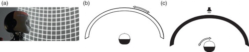
In order to show that our algorithm can train a network to handle real sensory data and reproduce natural behaviour found in humans, we conducted a similar experiment with a robot. Such biorobotic experiments are to provide an existential proof for sensorimotor conditions in which a given model can produce the theorised behaviour, and are one tool, along with analysis and simulations, for corroborating models in computational biology (Bauer, Dávila-Chacón, Strahl, & Wermter, 2012; Brooks, 1992; Datteri & Tamburrini, 2007; Rucci, Tononi, & Edelman, 1997). The robot, an iCub robotic head (Beira et al., 2006), was placed in our robotic virtual reality environment (Bauer, Dávila-Chacón et al., 2012). This environment allows us to present visual and auditory stimuli at various locations along a half-circle around the robot (Figure 2). In the following, we will describe the combined, spatially congruent auditory and visual stimuli we presented to the robot and how we pre-processed the sensory data to generate input for training our network. We will report on the system's performance when presented with auditory, visual, congruent audio–visual, and incongruent audio–visual data, and how that behaviour compares to the one observed by Alais and Burr (2004).

Figure 2. Experimental setup: (a) the iCub robotic head – a robotic head designed for experiments in developmental robotics (Beira et al., 2006) (in our robotic VR environment). (b) Recording of visual stimuli: the column of dots moves around the robot. This allows us to gather large numbers of visual data points quickly and produces slight location-dependent changes in the stimulus as in natural visual perception. (c) Recording of auditory stimuli: the robot rotates w.r.t. the speaker. This way, we were able to present stimuli with a density of 1° in an automated fashion.

3.1. Stimuli and training

Sensory signals reaching the integrative deep layers of the SC (dSC) are never raw. They are first shaped by the embodiment of and preprocessing in the sensory organs themselves, such as filtering and compression in retina and optic nerve (Marr, 1983; Stone, 2012), or semi-mechanical frequency decomposition in the cochlea (Slaney, 1993; Yates, Johnstone, Patuzzi, & Robertson, 1992). The signals are further changed before reaching the dSC by later stages of processing, like the visual superficial layers of the SC (sSC) (Wang, Sarnaik, Rangarajan, Liu, & Cang, 2010) and the inferior colliculus (IC), which integrates various auditory spatial cues (Schnupp et al., 2011, p. 205–209) and which is one major source of auditory information of the SC (DeBello & Knudsen, 2004; Edwards, Ginsburgh, Henkel, & Stein, 1979; May, 2006).

Any one model of visual and auditory input to the SC would be complex and species specific, and if we had had to commit to one specific model for generating input to our network from raw stimuli in our experiment, the validity of any claims derived from the experiment's results would be limited by the validity of that model. Fortunately, a strength of our model is that it explains how the dSC can learn to integrate information without built-in knowledge of the relationship between its input and the location of a stimulus. Therefore, our focus in choosing appropriate pre-processing of our stimuli was not so much on generating perfectly realistic SC input. Instead, we aimed to generate input which roughly preserved important properties of actual SC input (details described later), which was experimentally and computationally feasible to produce, and, in the case of visual input, whose reliability for localisation was easily modulated.

3.1.1. Visual stimuli

To emulate the important features of visual SC input in Alais and Burr (2004)’s experiment, we chose stimuli whose dominant property was their location and whose reliability could be manipulated to introduce significant uncertainty about that location.

Therefore, to generate a visual stimulus at angle α, we projected a column of dots against the screen which were randomly distributed around that angle α following a Gaussian distribution. Visual input activations for training and testing our network were generated from the images then taken by the robot as described in Figure 3. Reliability of the visual stimulus and computational complexity was tuned by empirically choosing appropriate numbers for the number of visual input neurons, the factor by which the mean intensities were scaled, and the height of the strips cut from the image. We chose 320 for the number of visual input neurons, 0.1 for the scaling factor, and, for training, 140 pixels for the height of the strips.

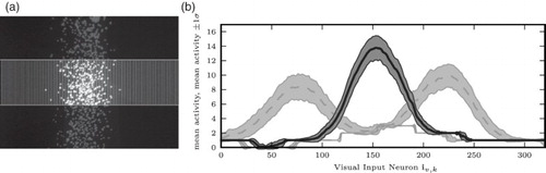
Figure 3. Visual input: (a) column of dots projected on the screen right in front of the robot. A horizontal strip (area between horizontal white lines) of the camera image is horizontally subsampled. The mean intensity of pixels in each vertical column of the subsampled strip is computed, scaled by 0.1, and reduced to the nearest integer (see (b)). (b) Visual input activity. Solid line: mean over all data points at α=0°. Dashed lines: mean over all data points at α=+10°, α=−10°. Grey backgrounds: mean±one standard deviation.

3.1.2. Auditory stimuli

Binaural recordings for auditory localisation were made by playing white noise on a speaker at a distance of about 1.30 m and rotating the robot wrt. the speaker. Auditory input activity was generated from these recordings using the IC model from (Dávila-Chacón et al., 2012). The IC is a midbrain region that performs auditory localisation by integrating input from the medial superior olive (MSO) and the lateral superior olive (LSO). The MSO responds to interaural time differences (ITDs) and can localise more accurately sounds with low-frequency components, whereas the LSO responds to interaural level differences (ILDs) and can localise more accurately sounds with high-frequency components. Therefore, integration of ITDs and ILDs in the IC allows the localisation of sounds across the entire audible spectrum. Since projections from the IC to the intermediate and dSC are a major source of auditory input to the SC (see above), the auditory input activity generated by the model described by Dávila-Chacón et al. (2012) is a reasonable approximation to the actual auditory input activity to the SC. For computational efficiency, auditory input was normalised by dividing each input activity ${\mathbf{\text{a}}}_{a,k,t}$ in auditory data point ${\mathbf{\text{a}}}_{a,t}={\mathbf{\text{a}}}_{a,0,t},{\mathbf{\text{a}}}_{a,1,t},\dots ,{\mathbf{\text{a}}}_{a,n_a,t}$ by the mean input $⟨{\mathbf{\text{a}}}_{a,k,m}{⟩}_m$ over all data points ${\mathbf{\text{a}}}_{a,m}$ (Figure 4).

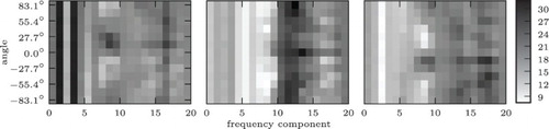
Figure 4. Mean auditory input for angles−15°, 0°, and 15°. IC activations are population codes of shape 20×13. Each column of neurons analyses a different frequency, each row prefers a different angle. See Dávila-Chacón et al. (2012) for details. Note that there is some regularity in the input, but it is fairly complex, relatively high-dimensional, and noisy (even when it is averaged as seen).

3.1.3. Training

In total, we collected 12,300 visual data points (300 per angle) and 19,660 auditory data points (476–480 per angle) at 41 angles between −20° and 20°.

Twenty percent of both visual and auditory data points were set aside for testing, leaving 9840 visual and 15,728 auditory data points for training. The rest was used to train the network. In each training and testing step, we randomly chose one whole angle α between −20° and 20° and randomly selected a visual and an auditory input activity for that angle, generated as described above. The input to our network was then the concatenation of these two activations into one vector of length $n_v+n_a=320+260=580=n_i.$ It is important to note at this point that the separation of the input population into visual and auditory sub-populations and the spatial relationship of neurons within the sub-populations are opaque to the output neurons: an output neuron o simply receives connections from a (logical) population of input neurons and makes no assumptions about the modality and the point in space from which the information conveyed by these input connections originates.

We trained the network over 40,000 training steps. With 9840 visual and 15,728 auditory data points belonging to only 41 classes, we did not expect or observe overfitting. Also, this study does not focus on the computational efficiency of our algorithm and in particular the speed of learning. We therefore chose a number of training steps at which we were sure that the network had arrived at a stable state. After training, we determined the mapping learned by the network: we first determined the BMUs for another 6000 data points, randomly selected from the training set. Then, we computed for all data points with the same BMU o the mean over the angles at which the constituent visual and auditory input activations had been recorded. That mean angle was then chosen as the preferred value $l_{\mathbf{\text{o}}}$ of the neuron o.

Then, to compute the accuracy of our network we presented it with 3000 data points from the test set. We took the preferred value $l_{{\mathbf{\text{o}}}_B}$ of the BMU ${\mathbf{\text{o}}}_B$ for each data point as the network's estimate of the true angle α at which the visual and auditory component of that data point were recorded (cross-sensory, congruent condition). To test the similarity between our network's behaviour and that of human beings, we also tested its performance with visual and auditory input alone (uni-sensory conditions).

Finally, to emulate incongruent multi-sensory input as in Alais & Burr,’s (2004) experiment, we presented the network with data points from one visual activation from an angle α_v and an auditory data point with an angle α_a, where α_a was ${\alpha }_a={\alpha }_v+5^{\circ }$ (cross-sensory, incongruent conditions).

3.2. Results

Figure 5 shows the spatial organisation of the network after training. Stimuli around the centre of the visual field are clearly mapped according to their topology. The first and the last neuron in the population attract stimuli from a range of stimuli at one end of the spectrum, each. This is due, in part, to stimuli in the periphery actually being harder to distinguish: Visual stimuli are spread over more pixels as they move towards the edge of the visual field. The effect is similar, although the reasons more complex, in auditory localisation (Middlebrooks & Green, 1991). Another reason for many stimuli at the side being mapped to the two outermost neurons is the border effect observable in other SOM-like algorithms (Kohonen, 2001, 2013).

Figure 5. Spatial organisation of the network. Grey scale encodes number of times an angle α was mapped to a neuron o while determining the mapping of stimulus positions to neurons.

In the uni-sensory and cross-sensory, congruent conditions, we found that the mean squared error (MSE) of the network given visual, auditory, and multi-sensory input was ${\sigma }_v^2={4.68}^{\circ }$, ${\sigma }_a^2={4.82}^{\circ }$, and ${\sigma }_{ms}^2={2.46}^{\circ }$, respectively. Given the uni-sensory MSEs σ_v and σ_a, the MLE model predicts a multi-sensory MSE of: ${\hat{\sigma }}_{ms}^2=\frac{1}{1/{\sigma }_v^2+1/{\sigma }_a^2}\simeq {2.38}^{\circ }.$ The difference can be explained by the relatively large errors of the network in the uni-sensory conditions caused by the border effect, which is stronger for stimuli with greater ambiguity (uni-sensory) than for relatively reliable stimuli (cross-sensory).

In the cross-sensory, incongruent condition, the stimulus was located on average $\overline{\delta }\simeq {2.13}^{\circ }$ right of the visual stimulus. The predicted offset for this condition is ${\delta }_{\mathrm{MLE}}\simeq {2.46}^{\circ }$.

4. Simulated biology, PDFs, and absolute performance

The experiment related in the last section shows that our model integrates visual and auditory information similar to humans on the behavioural level. As noted in the Introduction, to be considered a model of natural multi-sensory integration at the neural network level, a model also needs to exhibit neurophysiological phenomena occurring in natural multi-sensory integration. One aspect, topographic mapping, was already demonstrated in the last section. In this section, we will report on a simulation we have conducted, which was designed to demonstrate two other phenomena in SC neurophysiology which our model reproduces: the spatial principle and the principle of inverse effectiveness. In experiments with natural stimuli, these phenomena are partially overshadowed by artefacts due to the specific stimuli presented and, more importantly in our experiment, by border effects caused by the large localisation errors we intentionally introduced to demonstrate behavioural phenomena.

We will also show that our network not only integrates cross-sensory stimuli near-optimally, as demonstrated above, but also learns to compute PDFs over latent variables and encode them in a PPC as theorised in Section 2, and thus integrates all the information in its input near-optimally. This, too, is only possible in simulations, where ground truth and the response properties of the input neurons are fully known.

4.1. Stimuli and training

To emulate the different quality of information supplied to the SC by different modalities, we separated the input population of our network into two sub-populations, one for visual and one for auditory input (Figure 1). Each of the neurons in these populations had a preferred value l of the location L of a simulated stimulus. In each of the two populations, preferred values were evenly distributed across the range of possible values of L. All input neurons had Gaussian tuning functions. Noise was Poisson distributed, roughly simulating noise properties of actual biological neural responses (Tolhurst et al., 1983; Vogels et al., 1989). The differences between the modalities were (1) the width of the Gaussian tuning functions, (2) the gain of the Gaussian tuning functions, and (3) the number of input neurons in each of the two populations.

Thus, let ${\mathbf{\text{i}}}_1,{\mathbf{\text{i}}}_2,\dots ,{\mathbf{\text{i}}}_{n_m}$ be the input neurons for modality $m\in \{a,v\}$. Then, the preferred value of neuron ${\mathbf{\text{i}}}_l,1\le l\le n_m$, was $l_{{\mathbf{\text{i}}}_l}=(l-1)/(n_m-1)$ and the response of ${\mathbf{\text{i}}}_l$ was a stochastic function of the stimulus value l given by (5) ${\mathbf{\text{a}}}_{{\mathbf{\text{i}}}_l}\sim \mathrm{Pois}\left(g_m\ast \exp \left(-\frac{(l_{{\mathbf{\text{i}}}_l}-l{)}^2}{{\sigma }_m^2}\right)\right),$(5) where $g_m\in \{g_a,g_v\}$ and ${\sigma }_m\in \{{\sigma }_a,{\sigma }_v\}$ were the modality-specific gain and width of the tuning function, respectively. See Table 1 for the actual values of the parameters in our experiment.

Table 1.  Simulation parameters.

Input	nm	gm	σm
m=v	60	8	0.005
m=a	40	4	0.01
Output
Neurons (no)	500

These parameters were chosen so the input contained enough information to localise the stimuli with input from either modality alone with errors much smaller than the range of L (thus reducing border effects) while still producing a demonstrable error in multi-sensory localisation. The effects reported in Results and Discussion were robust, qualitatively, for a wide range of parameters.

We trained the network extensively over 20,000 steps in which we chose l randomly from the interval [0, 1] and generated input population responses according to the stochastic tuning functions described in Equation (5). We then determined the mapping of preferred values to output neurons by generating input for all values $l\in \{(p-1)/(10,000-1)|p=1,2,\dots ,10,000\}$. Figure 6 shows the BMU for each of these values. For each output neuron, we estimated the mean of all values l for which it was the BMU to be its preferred value. Next, we will describe the experiments and evaluations of the trained network.

Figure 6. Mapping of stimulus values to output neurons. Grey scale encodes the number of times a value of L (y-axis) was mapped to a neuron o (x-axis).

4.1.1. Simulated neurophysiology

Two of the most prominent hallmarks of multi-sensory integration on the neurophysiological side are the spatial principle and the principle of inverse effectiveness (Stein & Stanford, 2008). According to the spatial principle, the response of a neuron to stimuli in different senses is enhanced if they are both in the neuron's receptive field (RF) (in our case, if they originate from the same direction) and depressed if one of the stimuli is and the other is in the suppressive zone surrounding the RF. According to the principle of inverse effectiveness, the enhancement effect is strong for weak stimuli and weak for strong stimuli. We tested whether our network reproduces the spatial principle by generating input activities with different l_m for different modalities $m\in \{a,v\}$. To see whether our network also reproduces enhancement and the principle of inverse effectiveness, we generated congruent input again, this time varying the gains of the neurons’ tuning functions, g_a and g_v in Equation (5).

4.1.2. PDFs and near-optimality

It is straightforward to compute a discretised PDF over values of l from the input population response, given knowledge of the input statistics (Equation (5) and Table 1). To assess the performance of our algorithm, we compared it against that of an MLE based on the computed PDF. Again, we simulated input for values of L spaced evenly over the interval [0, 1]. We presented this input to the network and chose the mapping (see above) of the BMU as the network's estimate of l.

4.2. Results

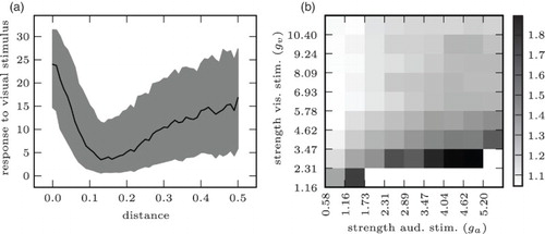
When presenting audio–visual stimuli with incongruent simulated auditory and visual locations p_a, p_v, we observed a clear cross-sensory depression effect: Figure 7(a) plots the mean response of that output neuron whose preferred value was l_v as a function of the absolute distance between the visual and the auditory stimulus |l_v−l_a|. It is clear that the strength of the response to the visual stimulus decreases as the auditory stimulus moves into the suppressive zone of the neuron whose preferred value is l_v. Enhancement and inverse effectiveness were apparent when presenting the network with congruent stimuli of varying intensity: Figure 7(b) shows the enhancement of the neural response to a visual stimulus as a function of the strength of an auditory stimulus. The figure clearly shows that the response to a weak visual stimulus is greatly enhanced by an auditory stimulus, but the response to a strong visual stimulus does not benefit as much.¹

Figure 7. The network reproduces principles of natural multisensory integration on the neurophysiological level: (a) depression and spatial principle. Strength of response to visual stimulus as a function of distance of auditory stimulus. (b) Enhancement and inverse effectiveness. Strength of response to (congruent) cross-sensory stimulus divided by strength of response to visual-only stimulus. White cells in lower right: response to auditory stimulus is stronger than to visual response (no enhancement of visual stimulus).

The network's ability to approximate and encode PDFs from noisy input is demonstrated in Figure 8. On congruent input, the network routinely produced activity similar to a PDF computed using knowledge of input response properties. To compare the network activity to the synthetic PDFs, we used normalised cross-correlation, as a measure of function similarity, and Kullback–Leibler (KL) divergence, as an information-theoretic measure of loss of information (Burnham & Anderson, 2002, p. 51). The mean normalised cross-correlation between the network activity and the synthetic PDFs sampled at the neurons’ preferred locations was 0.9247 (0.9598 for $\frac{1}{3}<l<\frac{2}{3}$). Mean KL divergence between the two was 153.4 bit, compared to a KL divergence of 2693 bit between the synthetic PDF and a uniform distribution (60.45 bit and 2216 bit for $\frac{1}{3}<l<\frac{2}{3}$).

Figure 8. The network generates a population code close to a synthetic PDF without prior knowledge of the input statistics: (a) incongruent input. First 60 (blue): visual input. Last 40 (red): auditory input. (b) Synthetic PDF. Right bump (red): PDF for aud. only input. Left bump (blue): PDF for vis. only input. Middle bump (black): PDF for full input. Vertical lines: ground truth (vis./aud.). (c) Network output. Right bump (red): Given aud. only input. Left bump (blue): Given vis. only input. Middle bump (black): Given full input. Vertical lines: ground truth (vis./aud.).

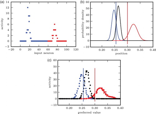
On incongruent input, activity similar to the synthetic PDF was produced whenever the simulated auditory and visual stimuli were within a certain distance from each other (as in the example shown in Figure 8). If they were far apart, the response to the combined, incongruent stimulus was most often similar to that to the visual stimulus alone.

The performance of our network was just a little below than that of an MLE based on the analytically computed PDF with an MSE of ${\sigma }_{\mathrm{network}}\simeq 1.120\times {10}^{-4}$ compared to ${\sigma }_{\mathrm{synth}.}\simeq 1.087\times {10}^{-4}$.

5. Discussion

The algorithm and network proposed in this paper are simple, yet we have shown that they can learn to localise stimuli from noisy multi-sensory data and that integration of multi-sensory stimuli then is comparable to MLE, which has also been shown for natural multi-sensory integration. We have demonstrated the network's ability to reproduce the formation of topographic multi-sensory maps, the spatial principle, and the principle of inverse effectiveness which are important aspects of multi-sensory integration in the SC (Stein & Meredith, 1993).

The network learns to approximately compute a PDF over the latent variable behind its input, and represent it in a PPC. Since the activity of a neuron therefore is the result of computing a PDF, the neurophysiological effects produced by the network are caused by statistical inference in multi-sensory neurons, as previously theorised by Anastasio, Patton, and Belkacem-Boussaid (2000).

There are a number of ways to remedy the border effect observed in the experiment and, less strongly, in the simulation. One could be using a network topology without borders, such as a spherical (actually: circular) or toroid topology (Ritter, 1999). This solution is theoretically interesting but not very attractive from a modelling perspective, as the SC does not have a border-free topology. Alternatively, a more complex training regime could help, in which only the innermost neurons are eligible as BMUs initially, with more and more neurons taking part as learning progresses (Ritter, 1999). A third mechanism which could alleviate the border effect could be adding Conscience (DeSieno, 1988), by which BMU selection is biased towards neurons which have not been BMU for many training steps. Applying the latter two mechanisms to our model and comparing them with actual SC physiology and especially development could be very interesting for future work. We did not use them here in order to keep our modeling simple.

Simulations in which auditory and visual positions were far apart showed that the network does not integrate such cross-sensory stimuli. Instead, the network roughly selects one of the uni-sensory stimuli, usually the strongest. This is a result of initialising the network's histograms with a small value ε and because of the early learning phase, in which each data point is used to update all neurons with considerable strength. For both reasons, every neuron learns to slightly over-estimate the probability of input activations which are very unlikely for their preferred value, but likely for others. To understand how this leads to the observed behaviour, consider the situation where the visual and auditory stimulus locations l_v and l_a are far apart. In this situation, the output neuron with the preferred value l_v overestimates the likelihood of seeing the current auditory input activity when a cross-modal stimulus is at location l_v. The strong evidence from visual input for the hypothesis that the stimulus is at l_v then outweighs the counter-evidence from auditory input and the network selects a position near l_v as the most likely location of the stimulus. Note that only the probablility of very unlikely input activities is significantly overestimated and the effect thus only occurs for grossly incongruent input.

The phenomenon described above may seem like an artefact at first, but it reflects a property of biological neurons and neural computation: realistic spiking behaviour cannot represent numerical values at arbitrary precision (in finite time, on a fixed range of values). Therefore, it would be tempting to see our network's behaviour in light of psychological findings showing that humans also systematically mis-estimate low probabilities (Ungemach, Chater, & Stewart, 2009). However, an even more compelling parallel to human behaviour comes from the ventriloquist effect: a visual stimulus and an auditory stimulus are perceived as one cross-sensory stimulus at one location in space if the actual distance between them is below a certain threshold. Otherwise, they are perceived as two uni-sensory stimuli at different locations (Jack & Thurlow, 1973). The similarity to our network's behaviour suggests a common cause: if part of the input is more likely caused by background noise or an additional stimulus than by the main stimulus, then it is effectively ignored. In the simulations reported here, the probability for some input being caused by another stimulus was determined by the training sequence. If input during training included baseline noise or multi-stimulus input, that probability would be superseded by a higher, learned probability of spurious input activity.² A prediction following from this analysis is that the strength of sensory noise during development determines the susceptibility to the ventriloquism effect. Xu et al. (2012) found that SC neurons in cats which are raised in extremely low-noise conditions³ develop low tolerance to spatial or temporal incongruency, integrating cross-sensory stimuli only within a small spatio-temporal window. Whether this effect varies systematically with ecological noise and what its effects are at the behavioural level remains to be seen.

Our model is not a model on the level of biological implementation. As we have mentioned, histograms as a method of approximating likelihood functions are not biologically plausible and we do not specify any particular methods for implementing divisive normalisation and winner selection. We see our model on the algorithmic level, in Marr,’s (1983) sense, akin for example to that due to Ohshiro, Angelaki, and DeAngelis (2011): it is situated between computational theories of multi-sensory integration, like the MLE model due to Alais and Burr (2004), and theories of hardware implementation like for example the one due to Cuppini, Magosso, Rowland, Stein, and Ursino (2012). In this position, it connects the interaction of the parts of the hardware implementation to the behaviour described by the mathematical theory and thus allows for predictions about what happens to the hardware if there are changes on the behavioural level, and vice versa.

That said, we believe that the operations used by our algorithm are simple enough to be implemented by a network of biological neurons. Divisive normalisation has explained many aspects of neural responses in sensory processing, and possible mechanisms have been identified (Carandini & Heeger, 2011). A literal implementation of histograms by neurons which count the times they observe a particular input activation at each of their synapses is implausible. However, neurons apparently encoding probabilistic variables, computed from sensory input, have been found (Yang & Shadlen, 2007) and Soltani and Wang (2010) have shown how neurons may learn to compute such variables from input using biologically plausible mechanisms. Extensions of Soltani and Wang's work are a promising direction for implementing the statistical computations necessary for our model to reach further into Marr,’s (1983) domain of hardware implementations. Such extensions are the subject of future work. In the meantime, our assumption, backed by results such as those from Yang and Shadlen (2007), is that neurons or neural microcircuits can gradually learn to compute likelihood functions from input. We use histograms to model this ability and propose that it may play a role together with self-organisation in learning multi-sensory integration.

If neural microcircuits possess this ability to compute likelihoods, and if self-organisation similar to the account in this study occurs, then that could explain how the PPC presupposed by studies such as those due to Beck et al. (2008), Cuijpers & Erlhagen (2008), and Fetsch et al. (2013) could come about. Like the models proposed by Ohshiro et al. (2011) and Fetsch et al. (2013), our model uses divisive normalisation and the neurophysiological effects it reproduces depend in part on that. Our model differs, however, in that input neurons whose activity is excitatory for some integrative output neurons can be directly inhibitive for others and that excitation and inhibition develop through learning of input statistics. In the divisive normalisation models cited above, such an inhibition may arise indirectly through normalisation, but direct inhibition is not considered. The presence of direct differential inhibition is thus a prediction by which to test our model against other models incorporating divisive normalisation.

Although the focus of this study is on modeling, there are a few things to note from an algorithmic perspective: first, our method has a few similarities with generative topographic mapping (GTM) (Bishop, Svensén, & Williams, 1998). Like GTM, our algorithm learns a non-linear, topographic latent-variable model of its input. This feature is inherited from the original SOM algorithm (Yin, 2007). What our algorithm shares with GTM and not with the original SOM algorithm is its probabilistic interpretation. Like GTM, our algorithm computes the probabilities of a set of hypotheses for the value of the latent variable causing the input. To do that, both learn the noise statistics of the input to correctly integrate information from each of the data dimensions. One benefit of our algorithm over GTM is that its assumptions on noise distributions are weaker. GTM in its original formulation assumes Gaussian noise (Bishop et al., 1998). It can be modified to accommodate different noise distributions, but their shape is fixed for each input dimension before learning. Most importantly in the present context, although the histograms used by our neurons to approximate input likelihood functions are not biologically plausible, we argue that the underlying principle is (see above). Also, unlike GTM, our algorithm in its current form is not a batch learning algorithm (though it could be made to be one) and therefore allows for continuous learning, which is plausible for natural learning.

A weakness of the current algorithm compared to GTM and to previous SOM-based algorithms is that it potentially requires more data to train: since it makes no assumptions on the distribution of noise – not even that this distribution be uni-modal – it cannot learn from a data point in which one of the input dimensions has value $\mathbf{\text{d}}=v$ about the probability of data points where ${\mathbf{\text{d}}}^{\prime }=v+\delta$ if v+δ is in a different histogram bin than v. This is different in the regular SOM and the variants due to Zhou et al. (2011) and Bauer, Weber et al. (2012) as well as in GTM, which all assume continuity of the noise distribution. This weakness, of course, is related to the algorithm's strength of being able to learn any noise distribution in principle, as long as that noise distribution is well discretised by the bins of the histograms and as long as enough data is available for training.

6. Conclusion

In this paper, we have shown that our network can be practically trained on diverse kinds of input, including actual sensory input, and that it reproduces neurophysiological phenomena observed in natural multi-sensory integration and that it integrates multi-sensory information similar to an MLE, as found for humans and other animals. This is consistent with our hypothesis that self-organised learning of the statistics of the activity of individual input neurons and using the knowledge of those statistics to integrate multi-sensory stimuli may be part of what happens during the maturation and operation of the biological SC. Doubtless, other mechanisms are at work as well: depending on species, rough topographic organisation and basic sensory and even multi-sensory processing can be shown to be present in the SC from the start (Stein, 2012). Genetic predisposition thus is likely involved. Furthermore, reward-dependent learning may play a role in learning multi-sensory integration (Weisswange, Rothkopf, Rodemann, & Triesch, 2011). Indeed, it would be surprising if the brain did not make use of feedback for its actions, when it is available, and learn semi-supervised.

What we have shown here is that unsupervised learning alone, specifically statistical self-organisation, can go a long way in explaining the phenomenon that is natural learning of and performing multi-sensory integration in the SC.

Funding

This work is funded in part by the DFG German Research Foundation [grant number 1247] – International Research Training Group CINACS (Cross-modal Interactions in Natural and Artificial Cognitive Systems).

Notes

^†http://www.informatik.uni-hamburg.de/WTM/

1. This is the reason Figure 7(a) does not show strong enhancement: the simulated stimuli there were strong and thus the response to the congruent stimulus was not enhanced significantly.

2. In this study, we opted to train without baseline noise and with single-stimulus input. We made this choice for the sake of simplicity and to optimally bring out the effects focused on, here.

3. Conditions in which all audio–visual stimuli were congruent and highly discernable.

References

- Alais D., & Burr D. (2004). The ventriloquist effect results from near-optimal bimodal integration. Current Biology, 14(3), 257–262. doi: 10.1016/j.cub.2004.01.029
- Anastasio T. J., Patton P., & Belkacem-Boussaid K. (2000). Using Bayes’ rule to model multisensory enhancement in the superior solliculus. Neural Computation, 12(5), 1165–1187. doi: 10.1162/089976600300015547
- Barber M. J., Clark J. W., & Anderson C. H. (2003). Neural representation of probabilistic information. Neural Computation, 15(8), 1843–1864. doi: 10.1162/08997660360675062
- Bauer J., Dávila-Chacón J., Strahl E., & Wermter S. (2012). Smoke and mirrors – Virtual realities for sensor fusion experiments in biomimetic robotics. The 2012 IEEE conference on multisensor fusion and integration for intelligent systems (MFI) (pp. 114–119). Hamburg: IEEE.
- Bauer J., Weber C., & Wermter S. (2012). A SOM-based model for multi-sensory integration in the superior colliculus. The 2012 international joint conference on neural networks (IJCNN) (pp. 1–8). Brisbane: IEEE.
- Bauer J., & Wermter S. (2013). Self-organized neural learning of statistical inference from high-dimensional data. In F. Rossi (Ed.), International joint conference on artificial intelligence (IJCAI) (pp. 1226–1232). Beijing: AAAI Press.
- Beck J. M., Ma W. J., Kiani R., Hanks T., Churchland A. K., Roitman J., … Pouget A. (2008). Probabilistic population codes for Bayesian decision making. Neuron, 60(6), 1142–1152. doi: 10.1016/j.neuron.2008.09.021
- Beira R., Lopes M., Praça M., Santos-Victor J., Bernardino A., Metta G., … Saltarén R. (2006). Design of the robot-cub (icub) head. The 2006 IEEE international conference on robotics and automation (ICRA 2006) (pp. 94–100). Orlando, FL: IEEE.
- Bishop C. M., Svensén M., & Williams C. K. I. (1998). GTM: The generative topographic mapping. Neural Computation, 10(1), 215–234. doi: 10.1162/089976698300017953
- Brooks R. A. (1992). Artificial life and real robots. In F. J. Varela & P. Bourgine (Eds.) Toward a practice of autonomous systems: Proceedings of the first European conference on artificial life (pp. 3–10). Cambridge, MA: MIT Press.
- Burnham K. P., & Anderson D. R. (2002). Model selection and multimodal inference – A practical information-theoretic approach (2nd ed.). New York: Springer.
- Carandini M., & Heeger D. J. (2011). Normalization as a canonical neural computation. Nature Reviews Neuroscience, 13(1), 51–62.
- Cuijpers R. H., & Erlhagen W. (2008). Implementing Bayes’ rule with neural fields. Proceedings of the 18th international conference on artificial neural networks, Part II (pp. 228–237). Berlin: Springer.
- Cuppini C., Magosso E., Rowland B. A., Stein B. E., & Ursino M. (2012). Hebbian mechanisms help explain development of multisensory integration in the superior colliculus: A neural network model. Biological Cybernetics, 106(11–12), 691–713. doi: 10.1007/s00422-012-0511-9
- Datteri E., & Tamburrini G. (2007). Biorobotic experiments for the discovery of biological mechanisms. Philosophy of Science, 74(3), 409–430. Retrieved from http://www.jstor.org/stable/10.1086/522095. doi: 10.1086/522095
- Dávila-Chacón J., Heinrich S., Liu J., & Wermter S. (2012). Biomimetic binaural sound source localisation with ego-noise cancellation. In A. E. P. Villa, W. Duch, P. Érdi, F. Masulli, & G. Palm (Eds.), Artificial neural networks and machine learning ICANN 2012 (Vol. 7552, pp. 239–246). Berlin: Springer.
- DeBello W. M., & Knudsen E. I. (2004). Multiple sites of adaptive plasticity in the owl's auditory localization pathway. The Journal of Neuroscience, 24(31), 6853–6861. doi: 10.1523/JNEUROSCI.0480-04.2004
- DeSieno D. (1988). Adding a conscience to competitive learning. IEEE international conference on neural networks, 1988 (pp. 117–124). San Diego, CA: IEEE.
- Edwards S. B., Ginsburgh C. L., Henkel C. K., & Stein B. E. (1979). Sources of subcortical projections to the superior colliculus in the cat. The Journal of Comparative Neurology, 184(2), 309–329. doi: 10.1002/cne.901840207
- Ernst M. O., & Banks M. S. (2002). Humans integrate visual and haptic information in a statistically optimal fashion. Nature, 415(6870), 429–433. doi: 10.1038/415429a
- Fetsch C. R., DeAngelis G. C., & Angelaki D. E. (2013). Bridging the gap between theories of sensory cue integration and the physiology of multisensory neurons. Nature Reviews Neuroscience, 14(6), 429–442. doi: 10.1038/nrn3503
- Frassinetti F., Bolognini N., & Làdavas E. (2002). Enhancement of visual perception by crossmodal visuo-auditory interaction. Experimental Brain Research, 147(3), 332–343. doi: 10.1007/s00221-002-1262-y
- Georgopoulos A. P., Schwartz A. B., & Kettner R. E. (1986). Neuronal population coding of movement direction. Science, 233(4771), 1416–1419. doi: 10.1126/science.3749885
- Gori M., Del Viva M., Sandini G., & Burr D. C. (2008). Young children do not integrate visual and haptic form information. Current Biology, 18(9), 694–698. doi: 10.1016/j.cub.2008.04.036
- Gori M., Sandini G., & Burr D. (2012). Development of visuo-auditory integration in space and time. Frontiers in Integrative Neuroscience, 6. Retrieved from http://journal.frontiersin.org/Journal/10.3389/fnint.2012.00077/full. doi: 10.3389/fnint.2012.00077
- Imai T., Sakano H., & Vosshall L. B. (2010). Topographic mapping – The olfactory system. Cold Spring Harbor Perspectives in Biology, 2(8), a001776. doi: 10.1101/cshperspect.a001776
- Jack C. E., & Thurlow W. R. (1973). Effects of degree of visual association and angle of displacement on the ‘ventriloquism’ effect. Perceptual and Motor Skills, 37(3), 967–979. doi: 10.2466/pms.1973.37.3.967
- Jazayeri M., & Movshon A. A. (2006). Optimal representation of sensory information by neural populations. Nature Neuroscience, 9(5), 690–696. doi: 10.1038/nn1691
- Kaas J. H. (1997). Topographic maps are fundamental to sensory processing. Brain Research Bulletin, 44(2), 107–112. doi: 10.1016/S0361-9230(97)00094-4
- King A. J. (2013). Multisensory circuits. Neural circuit development and function in the brain (pp. 61–73). Oxford: Academic Press.
- Kohonen T. (1982). Self-organized formation of topologically correct feature maps. Biological Cybernetics, 43(1), 59–69. doi: 10.1007/BF00337288
- Kohonen T. (2001). Self-organizing maps. Berlin: Springer.
- Kohonen T. (2013). Essentials of the self-organizing map. Neural Networks, 37, 52–65. doi: 10.1016/j.neunet.2012.09.018
- Landy M. S., Banks M. S., & Knill D. C. (2011). Ideal-observer models of cue integration. In J. Trommershäuser, K. Körding, & M. S. Landy (Eds.), Sensory cue integration (pp. 251–262). Oxford: Oxford University Press.
- Marr D. (1983). Vision: A computational investigation into the human representation and processing of visual information. New York, NY: Henry Holt & Company.
- May P. J. (2006). The mammalian superior colliculus: Laminar structure and connections. Progress in Brain Research, 151, 321–378. doi: 10.1016/S0079-6123(05)51011-2
- Middlebrooks J. C., & Green D. M. (1991). Sound localization by human listeners. Annual Review of Psychology, 42(1), 135–159. doi: 10.1146/annurev.ps.42.020191.001031
- Neil P. A., Chee-Ruiter C., Scheier C., Lewkowicz D. J., & Shimojo S. (2006). Development of multisensory spatial integration and perception in humans. Developmental Science, 9(5), 454–464. doi: 10.1111/j.1467-7687.2006.00512.x
- Ohshiro T., Angelaki D. E., & DeAngelis G. C. (2011). A normalization model of multisensory integration. Nature Neuroscience, 14(6), 775–782. doi: 10.1038/nn.2815
- Pouget A., Dayan P., & Zemel R. S. (2003). Inference and computation with population codes. Annual Review of Neuroscience, 26(1), 381–410. doi: 10.1146/annurev.neuro.26.041002.131112
- Ritter H. (1999). Self-organizing maps on non-Euclidean spaces. Kohonen maps (pp. 97–108).
- Rucci M., Tononi G., & Edelman G. M. (1997). Registration of neural maps through value-dependent learning: Modeling the alignment of auditory and visual maps in the barn owl's optic tectum. Journal of Neuroscience, 17(1), 334–352. Retrieved from http://www.jneurosci.org/cgi/content/abstract/17/1/334.
- Schnupp J., Nelken I., & King A. J. (2011). Auditory neuroscience: Making sense of sound. Cambridge, MA: MIT Press.
- Seung H. S., & Sompolinsky H. (1993). Simple models for reading neuronal population codes. Proceedings of the National Academy of Sciences, 90(22), 10749–10753. doi: 10.1073/pnas.90.22.10749
- Slaney M. (1993). An efficient implementation of the Patterson–Holdsworth auditory filter bank (Tech. Rep.). Apple Computer, Perception Group.
- Soltani A., & Wang X.-J. (2010). Synaptic computation underlying probabilistic inference. Nature Neuroscience, 13(1), 112–119. doi: 10.1038/nn.2450
- Stein B. E. (2012). Early experience affects the development of multisensory integration in single neurons of the superior colliculus. In B. E. Stein (Ed.), The new handbook of multisensory processing (pp. 589–606). Cambridge, MA: MIT Press.
- Stein B. E., & Meredith M. A. (1993). The merging of the senses (1st ed.). Cambridge, MA: MIT Press.
- Stein B. E., & Stanford T. R. (2008). Multisensory integration: Current issues from the perspective of the single neuron. Nature Reviews Neuroscience, 9(5), 406. doi: 10.1038/nrn2377
- Stone J. V. (2012). Vision and brain: How we perceive the world (1 ed.). Cambridge, MA: MIT Press.
- Tolhurst D. J., Movshon J. A., & Dean A. F. (1983). The statistical reliability of signals in single neurons in cat and monkey visual cortex. Vision Research, 23(8), 775–785. doi: 10.1016/0042-6989(83)90200-6
- Ungemach C., Chater N., & Stewart N. (2009). Are probabilities overweighted or underweighted when rare outcomes are experienced (rarely)? Psychological Science, 20(4), 473–479. doi: 10.1111/j.1467-9280.2009.02319.x
- Vogels R., Spileers W., & Orban G. A. (1989). The response variability of striate cortical neurons in the behaving monkey. Experimental Brain Research, 77(2), 432–436. doi: 10.1007/BF00275002
- Wang L., Sarnaik R., Rangarajan K., Liu X., & Cang J. (2010). Visual receptive field properties of neurons in the superficial superior colliculus of the mouse. Journal of Neuroscience, 30(49), 16573–16584. doi: 10.1523/JNEUROSCI.3305-10.2010
- Weisswange T. H., Rothkopf C. A., Rodemann T., & Triesch J. (2011). Bayesian cue integration as a developmental outcome of reward mediated learning. PLoS ONE, 6(7), e21575+. doi: 10.1371/journal.pone.0021575
- Xu J., Yu L., Rowland B. A., Stanford T. R., & Stein B. E. (2012). Incorporating cross-modal statistics in the development and maintenance of multisensory integration. Journal of Neuroscience, 32(7), 2287–2298. doi: 10.1523/JNEUROSCI.4304-11.2012
- Yang T., & Shadlen M. N. (2007). Probabilistic reasoning by neurons. Nature, 447(7148), 1075–1080. doi: 10.1038/nature05852
- Yates G. K., Johnstone B. M., Patuzzi R. B., & Robertson D. (1992). Mechanical preprocessing in the mammalian cochlea. Trends in Neurosciences, 15(2), 57–61. doi: 10.1016/0166-2236(92)90027-6
- Yin H. (2007). Learning nonlinear principal manifolds by self-organising maps. In A. N. Gorban, B. Kégl, D. C. Scrunch, & A. Y. Zinovyev (Eds.), Principal manifolds for data visualization and dimension reduction (pp. 68–95). Berlin: Springer.
- Zhou T., Dudek P., & Shi B. E. (2011). Self-organizing neural population coding for improving robotic visuomotor coordination. The 2011 international joint conference on neural networks (IJCNN) (pp. 1437–1444). San Jose, CA: IEEE.