Graph learning-based spatial-temporal graph convolutional neural networks for traffic forecasting

Abstract

Traffic forecasting is highly challenging due to its complex spatial and temporal dependencies in the traffic network. Graph Convolutional Neural Network (GCN) has been effectively used for traffic forecasting due to its excellent performance in modelling spatial dependencies. In most existing approaches, GCN models spatial dependencies in the traffic network with a fixed adjacency matrix. However, the spatial dependencies change over time in the actual situation. In this paper, we propose a graph learning-based spatial-temporal graph convolutional neural network (GLSTGCN) for traffic forecasting. To capture the dynamic spatial dependencies, we design a graph learning module to learn the dynamic spatial relationships in the traffic network. To save training time and computation resources, we adopt dilated causal convolution networks with a gating mechanism to capture long-term temporal correlations in traffic data. We conducted extensive experiments using two real-world traffic datasets. Experimental results demonstrate that the proposed GLSTGCN achieves superior performance than all state-of-art baselines.

Keywords:

• Graph convolutional neural network
• dynamic graph learning
• traffic speed prediction
• spatial-temporal data

1. Introduction

Traffic forecasting is a fundamental component in Intelligent Transportation Systems (ITS). Accurate traffic forecasting is of great significance to traffic control, traffic management, and traffic planning. However, traffic forecasting is a challenging task due to its complex spatial and temporal dependencies:

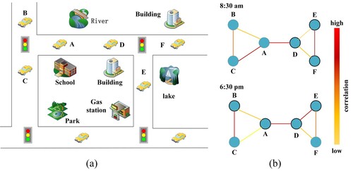
• Spatial dependency: The traffic conditions on a roadway are affected by the topological structure of the traffic network. The traffic conditions on the downstream roadways will be affected by traffic conditions of the upstream roadways through the transfer effect, and the traffic conditions on the upstream roadways will be affected by traffic conditions of the downstream roadways through the feedback effect (Dong et al., 2012). At the same time, spatial dependencies among roadways change over time. Figure 1 shows an example for illustration. As shown in Figure 1(b), the bold lines between two nodes represent their spatial correlation strength. The deeper the colour is, the closer the correlation is. We can observe that the correlation between node A and node C changes as time goes by.

• Temporal dependency: The traffic conditions change dynamically over time and will be affected by traffic conditions of previous moments and even longer earlier.

Figure 1. Dynamic spatial correlations between nodes. (a) Nodes in a road network. (b) Dynamic spatial correlations, node A and node C are not always highly correlated, although they are in the neighbourhood.

There has been a lot of work on traffic forecasting. The statistical model such as autoregressive integrated moving average (ARIMA) (Ahmed & Cook, 1979) and its variants (Lee & Fambro, 1999; Voort et al., 1996; Williams & Hoel, 2003) rely on the ideal stationary assumption that is not true in complicated real traffic dynamics. Traditional machine learning approaches, such as the k-nearest neighbour (k-NN) method (L. Zhang et al., 2013), support vector regression (SVR) (Chen et al., 2015) rely on the human-crafted features that need domain knowledge and is labouring.

With the development of deep learning, many deep learning-based approaches have been proposed. Recurrent neural network (RNN) and its variants (long short-term memory (LSTM) (Hochreiter & Schmidhuber, 1997) and gated recurrent unit (GRU) (Cho et al., 2014)) are widely used for traffic forecasting due to their excellent ability in learning temporal dependencies (Cui et al., 2018; Liao et al., 2018). Although RNN-based approaches can learn spatial dependencies, their structures are over-complex. In addition, RNN-based approaches have time-consuming iterations and the gradient vanishing problem in the case of long-term time sequence modelling. There are also methods that apply convolutional neural network (CNN) for traffic forecasting (Ma et al., 2017; J. B. Zhang et al., 2017). However, these single-type neural network models cannot deal with both spatial and temporal dependencies.

In order to capture both spatial and temporal dependencies, many hybrid neural network models that apply CNN for spatial feature learning and RNN for temporal features learning (Z. J. Lv et al., 2018; H. Yao et al., 2018). However, conventional CNNs are suitable for Euclidean space, such as images and regular grids. The traffic network has a complex topological structure and is essentially a graph structure.

Graph convolutional neural network (GCN) has become a natural choice for traffic forecasting as GCN can efficiently learn spatial features of data with irregular graph relationships based on spectral theory (Chung & Graham, 1997). Many approaches combine GCNs with CNNs (B. Yu et al., 2018) or RNNs (Geng et al., 2019; H. Yao et al., 2018; Zhao et al., 2019) to model temporal-spatial dependencies in traffic data. Although these GCNs based approaches have significantly improved traffic forecasting accuracy, they still have the following limitations.

First, these approaches adopt a fixed adjacency matrix in the graph convolutional network and lack the ability to modelling the dynamic change of the spatial relationships between roadways.

Second, these approaches are inefficient in capturing long-range temporal dependencies. RNN-based approaches are time-consuming for training and suffer from gradient vanishing for capturing long-range dependencies. CNN-based approaches can capture long-range dependencies but need to stack many layers because their receptive field size increases linearly with the number of stacked layers.

For overcoming these problems, we propose a graph learning-based spatial-temporal graph convolutional neural network (GLSTGCN) to more accurately predict network-wide traffic speed. Specifically, we design a graph learning module to learn the dynamic spatial relationships in the traffic network. At each time step, the graph learning module will learn a new adjacency matrix according to the current input data. Afterward, we apply the learned adjacency matrix to the graph convolutional layer to extract dynamic spatial features of traffic data. Inspired by WaveNet (Oord et al., 2016), we choose dilated causal convolutions to extract temporal features of traffic data. As the number of hidden layers and dilation factor increases, the receptive field size of dilated causal convolution networks increases exponentially. With the aforementioned components, GLSTGCN can efficiently deal with the long-range temporal and complex spatial dependencies for traffic forecasting. The main contributions of this work are summarised as follows:

• We propose a graph learning module to capture dynamic spatial dependencies in the traffic network. Specifically, the graph learning module learns an adjacency matrix according to the current inputs and the adjacency matrix changes dynamically with the inputs changes.

• We present an effective and efficient framework that combines the graph learning module, GCNs with dilated causal convolution networks to capture temporal and spatial dependencies simultaneously. The core idea is that we combine graph learning module with GCN to capture dynamic spatial dependencies, and adopt a dilated causal convolution network to capture long-range temporal dependencies that can reduce training time compared with RNN-based approaches and save computation resources compared with CNN-based approaches.

• We evaluate our proposed model on two real-world traffic datasets. The experiment results show that the proposed model outperforms all baselines with low computation costs.

The rest of the paper is organised as follows. We introduce the related work in Section 2 and background knowledge in Section 3. The details of the proposed model are described in Section 4. We evaluate the performance of the proposed model in Section 5. Finally, we summarise our work and plan the future work in Section 6.

2. Related work

Existing traffic forecasting approaches can be roughly classified into parametric approaches and nonparametric approaches. Parametric approaches include the time-series model, Kalman filtering model (Hinsbergen et al., 2012; Ojeda et al., 2013), and so on. The Autoregressive Integrated Moving Average (ARIMA) model (Hamed et al., 1995) is a popular time-series model. To improve prediction accuracy, different variants are proposed, such as subset ARIMA (Lee & Fambro, 1999), Kohonen ARIMA (Voort et al., 1996), seasonal ARIMA (Williams & Hoel, 2003), etc. These parametric approaches have simple algorithms and are convenient for computation. However, they have an ideal stationary assumption and can not deal with the nonlinearity and uncertainty characteristics of traffic data.

The nonparametric approaches can automatically learn statistical regularity from enough history traffic data. The early nonparametric approaches include the k-nearest neighbour (k-NN) method (L. Zhang et al., 2013), support vector regression (SVR) (Chen et al., 2015), the Bayesian network model (Sun et al., 2006) and so on. These early nonparametric approaches are traditional machine learning methods that require human-crafted features (Dai & Wang, 2021; Daid et al., 2021; Liu et al., 2021; Revathy et al., 2021). They need domain experts to extract features manually which is labouring and cannot fully reflect the traffic characteristics.

With deep learning becoming a hot research spot (Liang, Li, et al., 2021; Liang et al., 2020). Most recently, deep learning-based approaches receive more and more attention. Huang et al. (2014) proposed a traffic flow prediction method that combines a deep belief network with a multitask learning layer. Y. Lv et al. (2015) proposed a stacked autoencoder model to predict traffic flow. RNN and its variant LSTM were applied successfully in speech recognition, machine translation as their superior capability in modelling long-range sequences. They also have achieved good performance in traffic forecasting. Cui et al. (2018) proposed a deep-stacked bidirectional and unidirectional LSTM neural network architecture that can capture bidirectional temporal dependencies. Liao et al. (2018) proposed an LSTM-based encoder-decoder sequence learning framework, this approach took auxiliary information (e.g. social events, online crowd queries, etc) into account to facilitate the traffic speed prediction. However, those RNNs-based approaches have time-consuming iterations and do not learn spatial dependencies well. Different from the above RNNs-based approaches, we adopt dilated causal convolutional networks to deal with temporal dependencies in the traffic network to avoid time-consuming iterations.

CNNs are widely used to process images (Neena & Geetha, 2021; Srivastava & Biswas, 2020). There are also many approaches adopted CNNs to capture spatial dependencies in the traffic network. J. B. Zhang et al. (2017) employed three residual convolution networks to model the temporal closeness, period, and trend properties of crowd traffic and then combined the output of three networks with the external factors to predict the crowd traffic in each region. Ma et al. (2017) proposed a CNN-based method that learned traffic as images. Spatial-temporal dynamics were converted to images, a CNN was applied to these images to extract spatial and temporal features of traffic speed data. However, these single-type neural network models cannot deal with both spatial and temporal dependencies well.

To capture both spatial and temporal dependencies, many studies combined RNN and CNN. Z. J. Lv et al. (2018) combined RNN and CNN to learn meaningful time-series patterns that can reflect the traffic dynamics of the surrounding area. A look-up CNN was designed to learn spatial features, an RNN was used to learn temporal features. H. Yao et al. (2018) proposed a multi-view spatial-temporal network framework for demand prediction, which adopted an LSTM to capture temporal dynamics, a local CNN and semantic network embedding to capture spatial dependencies. To capture the irregular flows of urban traffic lines more effective, DU et al. designed an irregular CNN to learn the spatial features of the traffic passenger flows and utilised LSTMs to learn the temporal features (Du et al., 2020). The advantages of the CNN model in learning spatial features make it achieve great progress in traffic prediction tasks. However, CNN is more suitable for Euclidean space, such as images and grid data, rather than non-Euclidean space, such as graph structure data. Different from CNN-based approaches, we adopt GCN in this work.

The traffic network is essentially a graph structure. GCN is an appealing choice (Cui et al., 2019; Diao et al., 2019). B. Yu et al. (2018) proposed a novel deep learning framework that adopted GCN to extract spatial features and 1D CNN to extract temporal features of traffic data. Cui et al. (2019) proposed a traffic graph convolutional long short-term memory neural network to forecast the network-wide traffic state, which combined GCN and LSTM to learn the interactions between roadways in the traffic network. B. Yu et al. (2019) adopted a 3D graph convolutional network model to jointly learn spatial-temporal dependencies. Zhao et al. proposed a traffic prediction model which utilised GCN to capture spatial dependencies and GRU to capture temporal dependencies (Zhao et al., 2019). Wu et al. proposed a traffic speed prediction model which combined a self-adaptive adjacency matrix generation module with a predefined adjacency matrix to capture spatial dependencies and a dilated convolutional network to capture the temporal dependencies (Wu et al., 2019). However, these GCNs based approaches mostly adopted a fixed adjacency matrix which does not consider the dynamic change of the spatial relationships between roadways. To capture the dynamic spatial dependencies, Peng et al. proposed to use incident dynamic graph structures to model the dynamic station relationships (Peng et al., 2020). To overcome the data defects in traffic prediction, Peng et al. proposed to generate dynamic graphs by using reinforcement learning and GCN was applied on the dynamic graphs to learn dynamic spatial features (Peng et al., 2021). There are also attention-based traffic forecasting models which utilised attention mechanism (Bahdanau et al., 2014; Vaswani et al., 2017) to learn dynamic spatial dependencies. Guo et al. proposed an attention-based spatial-temporal forecasting model, which introduced attention to the STGCN model to learn dynamic spatial and temporal dependencies (Guo et al., 2019). Tang et al proposed a dynamic spatial and temporal graph attention network that utilised multihead attention to capture the dynamic spatial dependencies (Tang et al., 2020). However, attention-based approaches have a large number of trainable parameters which make the model training time-consuming and costs large memory resources. In this work, we propose a graph learning module to model the dynamic spatial relationships in the traffic network. The proposed graph learning module has a simple algorithm and the number of introduced parameters is low.

3. Preliminary

3.1. Graph convolutional neural networks

GCN is an extension of CNN from regular grids to irregular graphs and has achieved great performance in various tasks based on the graph structure. Existing GCNs can be classified into two categories. One is spectral domain-based graph convolution (Defferrard et al., 2016; Kipf & Welling, 2017) and the other is spatial domain-based graph convolution (Atwood & Towsley, 2016; Hamilton et al., 2017). Spectral graph convolution smoothes the features of nodes by spectral graph theory (Chung & Graham, 1997). Spatial graph convolution extracts the high-level features of a node by aggregating the features of its neighbour nodes. For signal $\mathbf{x}\in {\mathbf{R}}^N$, spectral graph convolution operator can be defined as (1) $\mathrm{\Theta }{\ast }_G\mathbf{x}=\mathbf{U}\mathrm{\Theta }(\mathbf{\Lambda }){\mathbf{U}}^T\mathbf{x},$(1) where $\mathbf{U}\in {\mathbf{R}}^{N\times N}$ is the matrix of eigenvectors of the normalised graph Laplacian $\mathbf{L}={\mathbf{I}}_N-{\mathbf{D}}^{-\frac{1}{2}}\mathbf{A}{\mathbf{D}}^{-\frac{1}{2}}=\mathbf{U}\mathbf{\Lambda }{\mathbf{U}}^T\in {\mathbf{R}}^{N\times N}$, ${\mathbf{I}}_N$ is the identity matrix, ${\mathbf{D}}_{ii}=\sum _j{\mathbf{A}}_{ij}$. To reduce the number of parameters and make the filter K-localised, the filter $\mathrm{\Theta }(\mathbf{\Lambda })$ can be designed as the Chebyshev polynomial $\mathrm{\Theta }(\mathbf{\Lambda })=\sum _{k=0}^{K-1}{\theta }_k{T}_k(\tilde{\mathbf{\Lambda }})$ with $\tilde{\mathbf{\Lambda }}=\frac{2}{{\lambda }_{\max }}\mathbf{\Lambda }-{\mathbf{I}}_N$ (${\lambda }_{\max }$ denotes the largest eigenvalue of $\mathbf{L}$), where $\theta \in {\mathbf{R}}^K$ is a vector of Chebyshev coefficients. Equation (1(1) $\mathrm{\Theta }{\ast }_G\mathbf{x}=\mathbf{U}\mathrm{\Theta }(\mathbf{\Lambda }){\mathbf{U}}^T\mathbf{x},$(1) ) can be rewritten as (2) $\mathrm{\Theta }{\ast }_G\mathbf{x}=\sum _{k=0}^{K-1}{\theta }_k{T}_k(\tilde{\mathbf{L}})\mathbf{x},$(2) where $\tilde{\mathbf{L}}=\frac{2}{{\lambda }_{\max }}\mathbf{L}-{\mathbf{I}}_N$, $T_k(\tilde{\mathbf{L}})\in {\mathbf{R}}^{N\times N}$ is the Chebyshev polynomial of order k (Defferrard et al., 2016).

It can be beneficial to reduce the number of parameters further and address overfitting, a first-order approximation of graph Laplacian is proposed (Kipf & Welling, 2017), the graph convolution can be defined as (3) $\mathrm{\Theta }{\ast }_G\mathbf{x}=\theta ({\tilde{\mathbf{D}}}^{-\frac{1}{2}}\tilde{\mathbf{A}}{\tilde{\mathbf{D}}}^{-\frac{1}{2}})\mathbf{x},$(3) where $\tilde{\mathbf{A}}={\mathbf{I}}_N+\mathbf{A}$, ${\tilde{\mathbf{D}}}_{ii}=\sum _j{\tilde{\mathbf{A}}}_{ij}$

3.2. Abbreviation list

For ease of reading, we have listed all the frequently used abbreviations in Table 1.

Table 1. The abbreviation list.

Abbreviation	Full name
CNN	Convolutional neural network
LSTM	Long short-term memory
GCN	Graph convolutional neural network
TCL	Temporal convolutional layer
GCL	Graph convolutional layer
GLSTGCN	Graph learning-based spatial-temporal graph convolutional network

4. Methodology

4.1. Problem definition

Traffic forecasting is a time-series prediction problem, we intend to forecast the future traffic speed by leveraging history traffic speed data. The traffic network can be treated as a graph $G=(V,E)$ where V is a set of $N=|V|$ nodes, each node represents a roadway, E is a set of edges each representing the connection between two nodes. These connections also can be described as a weighted adjacency matrix $\mathbf{A}\in {\mathbf{R}}^{N\times N}$, $A_{i,j}$ represents the strength of relationship between node i and j. The history traffic data can be represented as a time-series $[{\mathbf{x}}_{t-h+1},\dots ,{\mathbf{x}}_t]$, where ${\mathbf{x}}_t\in {\mathbf{R}}^{N\times 1}$ represents the traffic speed of N roadways at time t. With the aforementioned notations, the traffic forecasting problem can be defined as:

Given a graph G and the previous h time steps traffic speed of N roadways $[{\mathbf{x}}_{t-h+1},\dots ,{\mathbf{x}}_t]$, we aim to learn a function $f:{\mathbf{R}}^{N\times h}\to {\mathbf{R}}^{N\times p}$ which is able to forecast the next p time steps traffic speed, it can be represented as (4) $[{\mathbf{x}}_{t-h+1},\dots ,{\mathbf{x}}_t,G]\stackrel{f}{\to }{\mathbf{x}}_{t+1},\dots ,{\mathbf{x}}_{t+p}.$(4)

4.2. Overview of the proposed model

The architecture of the proposed GLSTGCN is shown in Figure 2, it includes a graph learning module, two graph learning-based spatial-temporal convolutional blocks (GLST-Conv Block), and an output layer. The graph learning module is used to model the dynamic spatial relationships in the traffic network. The structure of the graph learning module is presented in Figure 3. The spatial-temporal convolutional block is to learn complex spatial and temporal features in traffic data. It is a “sandwich” structure that includes two temporal convolutional layers (TCL) and a graph convolutional layer (GCL) in-between. The “sandwich” structure can help to reduce the model parameters and training time. The TCL is used to capture temporal dependencies and the GCL is used to capture spatial dependencies. The output layer includes a temporal convolutional layer and a fully connected layer. The out layer maps the output of the last spatial-temporal convolutional block to the final output $\mathbf{Y}={\mathbf{R}}^{N\times p}$, i.e. the next p time steps traffic speed of N roadways.

Figure 2. The architecture of GLSTGCN.

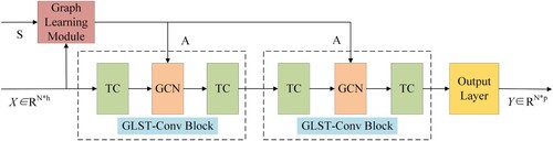
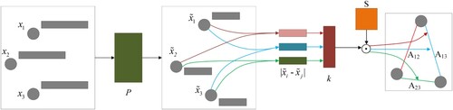
Figure 3. The architecture of graph learning module.

Next, we will give a detailed description of the graph learning module and the spatial-temporal convolutional block.

4.3. Graph learning module

The adjacency matrix is crucial for graph convolutional neural networks, it determines the receptive field of graph convolutional operation and the importance of the neighbourhood. An accurate adjacency matrix will improve traffic forecasting accuracy. In most existed approaches, the adjacency matrix of the traffic network is fixed. However, the spatial relationships between roadways change over time. Thus, a fixed adjacency matrix cannot reflect the spatial dependencies in the traffic network accurately. How to capture the dynamic spatial dependencies is a crucial problem.

Inspired by Jiang et al. (2019), this work proposes a graph learning module to learn the dynamic spatial relationships in the traffic network. According to the previous traffic speed data, the proposed graph learning module can learn an adjacency matrix to reflect the current spatial relationships in the traffic network. We will describe the dynamic adjacency matrix computation details of the graph learning module in the following section.

Given the traffic data for previous h time steps of N roadways $\mathbf{X}=({\mathbf{x}}_1,{\mathbf{x}}_2,\dots ,{\mathbf{x}}_N{)}^T\in {\mathbf{R}}^{N\times h}$, where ${\mathbf{x}}_i\in {\mathbf{R}}^h(i\in [1,N])$ is the speed sequences of roadway i, our purpose is to learn a nonnegative function ${\mathbf{A}}_{ij}=f({\mathbf{x}}_i,{\mathbf{x}}_j,\mathbf{S})$ that can represent current spatial relationship between roadway i and roadway j, where $\mathbf{S}\in {\mathbf{R}}^{N\times N}$ is the fixed adjacency matrix computed by geographical distance. Specifically, we learn $f({\mathbf{x}}_i,{\mathbf{x}}_j,\mathbf{S})$ via a single neural network, which is parameterised by a weight vector $\mathbf{k}=(k_1,k_2,\dots ,k_d{)}^T\in {\mathbf{R}}^{d\times 1}$.

Firstly, we multiply input data $\mathbf{X}$ by a projection matrix $\mathbf{P}\in {\mathbf{R}}^{h\times d}$ to preprocess the input data, (5) ${\tilde{\mathbf{x}}}_i={\mathbf{x}}_i\mathbf{P},\mathrm{for}i=1,2\dots N.$(5) Then, the preprocessed data and the fixed adjacency matrix S will be input to a single neural network to learn the current adjacency matrix. The theory behind the graph learning module is that if two roadways have close spatial dependencies, their speed sequences are similar. Thus, the output dynamic adjacency matrix of the graph learning module $\mathbf{A}$ is defined as (6) $\begin{array}{rl}{\mathbf{A}}_{ij}& =f({\tilde{\mathbf{x}}}_i,{\tilde{\mathbf{x}}}_j,\mathbf{S})\\ & =\frac{{\mathbf{S}}_{ij}\exp (ReLU({\mathbf{k}}^T|{\tilde{\mathbf{x}}}_i-{\tilde{\mathbf{x}}}_j|))}{\sum _{r=1}^{r=N}{\mathbf{S}}_{ir}\exp (ReLU({\mathbf{k}}^T|{\tilde{\mathbf{x}}}_i-{\tilde{\mathbf{x}}}_r|))},\end{array}$(6) where $ReLU(x)=max(0,x)$ is an activation function that guarantees ${\mathbf{A}}_{ij}⩾0$. The elements of weight vector $\mathbf{k}$ are learnable parameters. The more similar between the speed sequences of roadways i and j, the value $A_{ij}$ is bigger. The softmax function is used to guarantee the row sum of $\mathbf{A}$ is 1, (7) $\sum _{j=1}^{j=N}{\mathbf{A}}_{ij}=1,{\mathbf{A}}_{ij}⩾0.$(7) The fixed adjacency matrix $\mathbf{S}\in {\mathbf{R}}^{N\times N}$ is computed by geographical distance, it can be computed as (8) ${\mathbf{S}}_{ij}=\{\begin{array}{ll}\exp (-{\displaystyle \frac{d_{ij}^2}{{\sigma }^2}}),& i\ne j\mathrm{and}\exp (-{\displaystyle \frac{d_{ij}^2}{{\sigma }^2}})\ge ϵ\\ 0,& \mathrm{otherwise},\end{array}$(8) where ${\mathbf{S}}_{ij}$ is the weight of the edge between roadway i and j, $d_{ij}$ is the geographical distance between roadway i and j. ${\sigma }^2$ and ϵ are the thresholds to control the distribution and sparsity of the adjacency matrix.

4.4. Graph learning-based spatial-temporal convolutional block

In our framework, we adopt a graph learning-based spatial-temporal convolutional block to process graph-structured time-series and jointly capture long-range temporal dependencies and dynamic spatial dependencies in the traffic network. To extract the high-level time features of all time steps and the high-level spatial features of nodes in the multi-hop range, we stack two GLST-Conv Blocks. The GLST-COnv Block includes two temporal convolutional layers and a spatial convolutional layer as shown in Figure 2.

4.4.1. Temporal convolutional layer

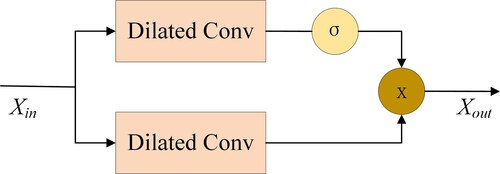
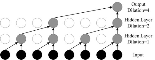
To learn the temporal features of traffic data, we propose a temporal convolutional layer. As opposed to RNNs-based approaches, dilated causal convolution networks do not have recurrent connections, which alleviate the gradient vanishing problem and save training time. Compared with CNNs-based approaches, dilated causal convolution networks can capture long sequences with less stacked layers, which saves computation resources. As shown in Figure 4, we adopt a dilated causal convolution network (Oord et al., 2016) combined with a gated mechanism (Dauphin et al., 2017) in our temporal convolution layer to capture the long-range temporal dependencies in the traffic network.

Figure 4. The architecture of temporal convolutional layer.

The dilated causal convolution network can increase the receptive field exponentially as shown in Figure 5. A dilated convolution network can be considered as the filter slides over an input sequence by skipping input values with a certain step. Given an input $\mathbf{x}\in {\mathbf{R}}^N$ and a filter $\mathbf{f}\in {\mathbf{R}}^m$, the dilated causal convolution of $\mathbf{x}$ with $\mathbf{f}$ at step t can be expressed as (9) $\mathbf{x}\ast \mathbf{f}(t)=\prod _{s=0}^{m-1}\mathbf{f}(s)\times \mathbf{x}(t-d\times s),$(9) where d is the dilation factor that controls the skipping steps.

Figure 5. A stacked of dilated causal convolutional layers with kernel size 2.

Given the input of temporal convolutional layer ${\mathbf{X}}_{in}\in {\mathbf{R}}^{t\times s})$, where t, s present temporal, spatial dimension, respectively. The output of temporal convolution layer can be defined as (10) $\mathrm{\Gamma }\ast \tau {\mathbf{X}}_{in}=({\mathbf{K}}_1\ast {\mathbf{X}}_{in})\odot \sigma ({\mathbf{K}}_2\ast {\mathbf{X}}_{in}),$(10) where ${\mathbf{K}}_1$, ${\mathbf{K}}_2$ are temporal convolutional kernels, ⊙ denotes element-wise product. The sigmoid function $\sigma (\cdot )$ controls which input of the current status are relevant for discovering compositional structure and dynamic variances in time-series.

4.4.2. Graph convolutional layer

To learn the spatial features of traffic data, we propose a graph convolutional layer. The graph convolutional layer is a graph convolutional nueral network which adopts the first approximation (Kipf & Welling, 2017) of the Chebyshev spectral filter (Defferrard et al., 2016). Let $\tilde{\mathbf{A}}\in {\mathbf{R}}^{N\times N}$ denotes the normalised adjacency matrix with self-loops of the learned dynamic adjacency matrix, $\mathbf{X}\in R^{N\times h}$denotes the input data, $\mathbf{Z}\in {\mathbf{R}}^{N\times p}$ denotes the output, and $\mathbf{W}\in {\mathbf{R}}^{h\times p}$ denotes the model parameter matrix, the output of the graph convolutional layer can be defined as (11) $\mathbf{Z}=\tilde{\mathbf{A}}\mathbf{X}\mathbf{W}.$(11) where $\tilde{\mathbf{A}}={\tilde{\mathbf{D}}}^{-\frac{1}{2}}\hat{A}{\tilde{\mathbf{D}}}^{-\frac{1}{2}}$, $\hat{A}={\mathbf{I}}_N+\mathbf{A}$, ${\tilde{\mathbf{D}}}_{ii}=\sum _j{\hat{\mathbf{A}}}_{ij}$.

4.5. Loss function

Existing approaches mostly generate multiple steps prediction via step-by-step iteration. Small errors in earlier time steps will lead to big errors in the latter time steps. To reduce long-term traffic forecast error, we choose to generate multiple time steps predictions at once. As $L1$ loss is robust during the training process, we use $L1$ loss as the training objective of the traffic forecasting task. Thus, the loss function of traffic forecasting can be written as (12) $L_{pre}=\sum _{i=1}^{i=p}\sum _{j=1}^{j=N}|{\tilde{\mathbf{x}}}_j^{t+i}-{\mathbf{x}}_j^{t+i}|,$(12) where ${\tilde{\mathbf{x}}}_j^{t+i}$ denotes the prediction value, ${\mathbf{x}}_j^{t+i}$ is the ground truth.

4.6. Algorithm of the proposed model

According to the above operations, Algorithm 1 shows the overall process to train the proposed model.

5. Experiments

In this section, we will compare the proposed GLSTGCN with other state-of-art baselines for traffic speed forecasting. We conduct experiments on two real-world datasets and illustrate the results of the experiments comprehensively.

5.1. Datasets

We verify our model on two real-world large-scale datasets, PEMS (B. Yu et al., 2018) and NYC (Diao et al., 2019), which are collected from the monitoring of traffic in California and New York City, respectively.

PEMS: This traffic dataset was collected from Caltrans Performance Measurement System (PEMS) by over 39,000 sensor stations. We select 228/142 stations among District 7 of California and collect data on weekdays of May and June of 2012.

NYC: This traffic dataset was collected from traffic speed detectors deployed on roads of the Manhattan District in New York. We select 50 sensors and 36 days of data range from 5th December 2017 to 9th January 2018.

The missing data are preprocessed by linear interpolation. All the data are aggregated into 5 min intervals, thus there are 288 data points of each roadway every day. Both datasets are divided into training sets, validation sets and test sets. And the input data are normalised by Z-score normalisation.

5.2. Experimental setup

The experiments were conducted on a Linux server under a computer environment with one Intel (R) Core (TM) i9-9900KS CPU @ 4 GHZ and one NVIDIA GeForce GTX 2080 GPU card. All the tests use 60 min of historical data to forecast the traffic speed in the next 15, 30, 45 min.

5.3. Evaluation metrics and baselines

To compare the performance of different methods, we adopt Mean Absolute Error (MAE) and Rooted Mean Square Error (RMSE) to evaluate the difference between the real traffic speed $x_j^{t+i}$ and the predicted speed ${\tilde{x}}_j^{t+i}$. (13) $\begin{array}{rl}MAE& =\frac{1}{Np}\sum _{i=1}^{i=p}\sum _{j=1}^{j=N}|{\tilde{\mathbf{x}}}_j^{t+i}-{\mathbf{x}}_j^{t+i}|\end{array}$(13) (14) $\begin{array}{rl}RMSE& =\sqrt{\frac{1}{Np}\sum _{i=1}^{i=p}\sum _{j=1}^{j=N}({\tilde{\mathbf{x}}}_j^{t+i}-{\mathbf{x}}_j^{t+i}{)}^2}\end{array}$(14) We compare our method with the following baselines:

• HA: Historical Average, it model the traffic speeds as a seasonal process. We use the average of the last 12 seasons as the prediction result.

• FNN: Feed-Forward Neural Network.

• DCRNN: Diffusion Convolutional Recurrent Neural Network applies graph convolution network into the recurrent neural network, and adopt a sequence-to-sequence architecture for traffic forecasting (Li et al., 2018);

• STGCN: Spatial-temporal Graph Convolutional Networks utilises graph convolution layer to extract spatial features and 1D convolution layer to extract temporal features (B. Yu et al., 2018);

• Graph WaveNet: Graph WaveNet adopts graph convolutional networks to learn spatial features and dilated causal convolution networks to learn temporal features of traffic data (Wu et al., 2019).

• ASTGCN: Attention-based Spatial and temporal graph convolutional networks introduce attention mechanism into the STGCN model. Only the recent component is taken to ensure fairness (Guo et al., 2019).

All these deep learning models are trained for 50 epochs, the batch size is set to 50 and use the hyperparameters provided by the authors. The model uses an Adam optimiser. The initial learning rate is 0.001 with a decay rate of 0.7 after every 5 epochs. The graph convolution kernel size is 3. the temporal convolution kernel sizes of two spatial-temporal convolution blocks are 3, 2, respectively. The dilation factors of two temporal convolution layers in each spatial-temporal convolution block are 1, 2, respectively. The output channels of three layers in the spatial-temporal convolutional block are 64, 16, 64, respectively.

5.4. Experiment results

Table 2 shows the comparisons of the proposed method and baselines for 15, 30, 45 min ahead prediction on datasets PEMS and NYC. Our proposed method outperforms all baselines by achieving the lowest MAE and RMSE on both datasets.

Table 2. Forecasting accuracy given by MAE and RMSE on dataset PEMS and NYC (15/30/45 min).

		15 min		30 min		45 min
Datasets	Model	MAE	RMSE	MAE	RMSE	MAE	RMSE
PeMS228	HA	9.3	13.13	9.3	13.13	9.3	13.13
	FNN	2.55	4.5	3.87	6.36	4.49	7.7
	DCRNN	2.34	4.3	3.25	6.15	3.95	7.42
	STGCN	2.24	4.08	3.07	5.78	3.68	6.94
	Graph WaveNet	2.32	4.43	3.26	6.43	3.99	7.79
	ASTGCN	2.46	4.37	3.33	6.02	3.93	7.02
	GLSTGCN	2.12	3.96	2.77	5.4	3.19	6.28
PeMS142	HA	9.42	13.16	9.42	13.16	9.42	13.16
	FNN	2.65	4.45	3.68	6.38	4.6	7.75
	DCRNN	2.29	4.29	3.21	6.18	3.86	7.5
	STGCN	2.25	4.06	3.09	5.77	3.66	6.88
	Graph WaveNet	2.34	4.45	3.3	6.5	4.05	7.91
	ASTGCN	2.56	4.55	3.48	6.28	4.1	7.34
	GLSTGCN	2.14	4	2.8	5.47	3.22	6.36
NYC	HA	3.99	5.5	3.99	5.5	3.99	5.50
	FNN	3.85	5.16	4.12	5.49	4.4	5.81
	DCRNN	2.95	4.22	3.13	4.51	3.29	4.72
	STGCN	2.7	4.05	2.89	4.35	3.09	4.62
	Graph WaveNet	2.93	4.2	3.11	4.43	3.27	4.67
	ASTGCN	2.72	4.04	2.88	4.28	3.03	4.48
	GLSTGCN	2.61	3.95	2.75	4.17	2.87	4.35

The traditional linear prediction method HA performs worst due to its simple algorithm and incapability to deal with nonlinear temporal dynamics and complex spatial dependencies in the traffic data. The neural network method FNN gets better results than the traditional linear prediction method. But FNN cannot model spatial dependencies which makes it cannot get satisfactory prediction accuracy. Graph convolutional neural network methods (e.g. DCRNN, STGCN, Graph WaveNet, ASTGCN and GLSTGCN) all achieve better performance which demonstrates the importance of simultaneously learning complex temporal and spatial dependencies in the traffic network. DCRNN and STGCN use a predefined adjacency matrix to model spatial dependencies in the traffic network, they cannot capture the dynamic spatial relationships between roadways. Although Graph WaveNet uses an adaption adjacency matrix combined with a predefined adjacency matrix to model spatial relationships between roadways, it still can not model dynamic spatial relationships. ASTGCN learns dynamic spatial dependencies with attention mechanism, but it performs not well. The proposed GLSTGCN achieves the best performance among all methods as it efficiently captures the dynamic spatial dependencies and temporal dependencies in the traffic network.

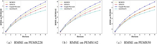
Figures 6 and 7 further shows the prediction results at each horizon on datasets PEMS and NY. As we can see, as the prediction horizon becomes longer, the prediction performance goes down for all methods. Compared with the baselines, the prediction performance of the proposed method degrades slowly when the prediction horizon becomes longer. GLSTGCN performs well for both short-term and long-term prediction and obtains better MAE and RMSE for almost all horizons.

Figure 6. Prediction MAE of different methods on each horizon on the dataset.

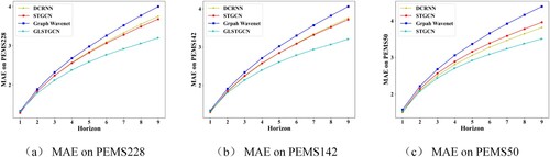
Figure 7. Prediction RMSE of different methods on each horizon on the dataset.

5.5. Effect of graph learning module

We conduct experiments with two different configurations on dataset PEMS and NYC to verify the effectiveness of the proposed graph learning module. The first one uses the predefined adjacency matrix to model spatial dependencies which do not have the graph learning module, the second one is the proposed GLSTGCN. Table 3 shows the test MAE and test RMSE for 15/30/45 min ahead prediction. To verify the credibility of the results, we ran experiments with two configurations 5 times on dataset PEMS228 respectively, the fluctuation of MAE for 15/30 min was within 0.01, and the fluctuation of MAE for 45 min was within 0.02. The experiment results show that the proposed GLSTGCN gets better prediction accuracy which indicates the importance of learning dynamic spatial dependencies for traffic prediction.

Table 3. The effect of graph learning module.

Data	Model	MAE(15/30/45 min)	RMSE(15/30/45 min)
PEMS-228	Distance Graph	2.17/2.82/3.28	4.06/5.49/6.35
	GLSTGCN	2.14/2.78/3.18	3.98/5.39/6.19
PEMS-142	Distance Graph	2.16/2.81/3.24	4.02/5.45/6.31
	GLSTGCN	2.14/2.78/3.19	3.97/5.37/6.21
NYC	Distance Graph	2.70/2.87/3.03	4.14/4.42/4.64
	GLSTGCN	2.68/2.85/3.01	4.12/4.38/4.6

5.6. Parameter selection

To evaluate the effect of a different number of hidden units in the graph learning module, we conduct experiments on dataset PEMS and NYC to test the prediction performance of the proposed model with a different number of hidden units. As shown in Tables 4, 5 and 6. We get the most worse prediction accuracy when the number of hidden unit is set to 5. And the prediction accuracy changes slightly with the number of hidden units greater than 10. The possible reason is that the feature dimension of the input data of the graph learning module is 12. It doesn't make much sense to choose more hidden units. Considering the prediction performance and the computation cost, we set the number of hidden units to 10 in this paper.

Table 4. Test MAE and RMSE versus the number of hidden units in the graph learning module (PEMS228).

	15 min		30 min		45 min
Dimension	MAE	RMSE	MAE	RMSE	MAE	RMSE
5	2.13	4	2.78	5.44	3.19	6.31
10	2.12	3.96	2.77	5.4	3.19	6.28
20	2.13	3.96	2.77	5.39	3.19	6.27
30	2.14	3.97	2.77	5.38	3.18	6.25
40	2.13	3.94	2.76	5.35	3.17	6.19
50	2.13	3.95	2.76	5.35	3.17	6.2

Table 5. Test MAE and RMSE versus the number of hidden units in the graph learning module (PEMS142).

	15 min		30 min		45 min
Dimension	MAE	RMSE	MAE	RMSE	MAE	RMSE
5	2.16	4.03	2.82	5.53	3.26	6.42
10	2.14	4	2.8	5.47	3.22	6.36
20	2.15	3.99	2.8	5.47	3.22	6.37
30	2.15	3.97	2.8	5.47	3.21	6.36
40	2.15	3.98	2.8	5.46	3.23	6.36
50	2.15	3.98	2.8	5.46	3.23	6.35

Table 6. Test MAE and RMSE versus the number of hidden units in the graph learning module (PEMS50).

	15 min		30 min		45 min
Dimension	MAE	RMSE	MAE	RMSE	MAE	RMSE
5	2.47	4.4	3.16	5.85	3.6	6.74
10	2.46	4.37	3.11	5.79	3.54	6.66
20	2.45	4.37	3.11	5.8	3.55	6.67
30	2.44	4.34	3.11	5.79	3.55	6.66
40	2.45	4.36	3.12	5.8	3.57	6.67
50	2.46	4.36	3.12	5.81	3.56	6.66

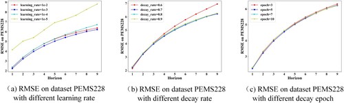
To validate the rationality of the hyperparameter settings, we conduct experiments with different settings on the dataset PEMS228. The prediction results of different hyperparameter settings are shown in Figures 8 and 9. From Figures 8(a) and 9(a), we can find that the lowest MAE and RMSE are achieved when the learning rate is 0.001. From Figures 8(b) and 9(b), we can see that the MAE and RMSE change slightly with decay rate, and get the lowest MAE and RMSE when the decay rate is 0.7. From Figures 8(c) and 9(c), we also find that the MAE and RMSE change slightly with decay frequency (i.e. decay after how many epochs), and get the lowest MAE and RMSE when the decay frequency is 5.

Figure 8. Prediction MAE on dataset PEMSE228 with different hyperparameter settings.

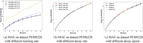
Figure 9. Prediction RMSE on dataset PEMSE228 with different hyperparameter settings.

5.7. Computation cost

We compare the computation cost of the proposed method with GCGRU and STGCN on dataset PEMS and NYC. As shown in Table 7, in training, GLSTGCN runs 7 times faster than GCGRU at least and a little faster than STGCN. For the test, we measure the total time of each model on the test data. GLSTGCN has the lowest computation time. This is because we generate 9 predictions in one run while GCGRU has to produce the results step-by-step. Besides, GCGRU has time-consuming recurrent connections.

Table 7. Computation cost.

		Computation time
Data	Models	Training(s/epoch)	Test(s)
PEMS-228	DCRNN	4369.02	662.82
	STGCN	200.15	95.39
	GLSTGCN	184.52	9.62
PEMS-142	DCRNN	1720.33	294.78
	STGCN	125.29	58.25
	GLSTGCN	107.52	6.38
NYC	DCRNN	221.07	24.36
	STGCN	36.94	17.61
	GLSTGCN	32.25	2.47

6. Conclusion and future work

In this paper, we propose a graph learning-based spatial-temporal graph convolution neural network (GLSTGCN) for traffic forecasting. We propose a graph learning module to learn the dynamic spatial relationships according to the current input in the traffic network. The proposed GLSTGCN can capture long-range temporal and complex spatial dependencies efficiently and effectively. Experiments show that our model achieves state-of-art results on both two real-world datasets. In future work, we will further optimise the network structure and combine it with other deep learning methods to learn the dynamic spatial dependencies to improve prediction accuracy.

Disclosure statement

No potential conflict of interest was reported by the author(s).

Additional information

Funding

The work was supported by the National Natural Science Foundation of China [grant number 61976087]  and the National Natural Science Fund for Distinguished Young Scholars (grant number  62025201)

References

- Ahmed, M. S., & Cook, A. R. (1979). Analysis of freeway traffic time-series data by using Box-Jenkins techniques. Transportation Research Record Journal of the Transportation Research Board, 773(722), 1–9.
- Atwood, J., & Towsley, D. (2016). Diffusion-convolutional neural networks. In Advances in neural information processing systems (pp. 1993–2001). Morgan Kaufman.
- Bahdanau, D., Cho, K., & Bengio, Y. (2014). Neural machine translation by jointly learning to align and translate. In 3rd International conference on learning representations, ICLR. OpenReview.net.
- Chen, R., Liang, C. Y., Hong, W. C., & Gu, D. X. (2015). Forecasting holiday daily tourist flow based on seasonal support vector regression with adaptive genetic algorithm. Applied Soft Computing, 26, 435–443. https://doi.org/10.1016/j.asoc.2014.10.022
- Cho, K., Merrienboer, B. V., Gulcehre, C., Bahdanau, D., Bougares, F., Schwenk, H., & Bengio, Y. (2014). Learning phrase representations using RNN encoder-decoder for statistical machine translation. In Proceedings of the 2014 conference on empirical methods in natural language processing (pp. 1724–1734). ACL.
- Chung, F. R. K., & Graham, F. C. (1997). Spectral graph theory. American Mathematical Soc.
- Cui, Z. Y., Henrickson, K., Ke, R. M., & Wang, Y. H. (2019). Traffic graph convolutional recurrent neural network: A deep learning framework for network-scale traffic learning and forecasting. IEEE Transactions on Intelligent Transportation Systems, 21(11), 4883–4894. https://doi.org/10.1109/TITS.2019.2950416
- Cui, Z. Y., Ke, R. M., Pu, Z. Y., & Wang, Y. H. (2018). Deep bidirectional and unidirectional LSTM recurrent neural network for network-wide traffic speed prediction. Preprint. arXiv:1801.02143
- Dai, Y. H., & Wang, T. (2021). Prediction of customer engagement behaviour response to marketing posts based on machine learning. Connection Science, 33(4), 891–910. https://doi.org/10.1080/09540091.2021.1912710
- Daid, R., Kumar, Y., Hu, Y. C., & Chen, W. L. (2021). An effective scheduling in data centres for efficient CPU usage and service level agreement fulfilment using machine learning. Connection Science, 33(4), 954–974. https://doi.org/10.1080/09540091.2021.1926929
- Dauphin, Y. N., Fan, A., Auli, M., & Grangier, D. (2017). Language modeling with gated convolutional networks. In International conference on machine learning (pp. 933–941). PMLR.
- Defferrard, M., Bresson, X., & &Vandergheynst, P. (2016). Convolutional neural networks on graphs with fast localized spectral filtering. In Advances in neural information processing systems (pp. 3837–3845). Morgan Kaufman.
- Diao, Z. L., Wang, X., Zhang, D. F., Liu, Y. R., Xie, K., & He, S. Y. (2019). Dynamic spatial-temporal graph convolutional neural networks for traffic forecasting. In Proceedings of the AAAI conference on artificial intelligence (Vol. 33, pp. 890–897). AAAI Press.
- Dong, C. J., Shao, C. F., Zhuge, C. X., & Meng, M. (2012). Spatial and temporal characteristics for congested traffic on urban expressway. Journal of Beijing University of Technology, 38(8), 1242–1246.
- Du, B. W., Peng, H., Wang, S. Z., Bhuiyan, M. Z. A., Wang, L. H., Gong, Q. R., Liu, L., & Li, J. (2020). Deep irregular convolutional residual LSTM for urban traffic passenger flows prediction. IEEE Transactions on Intelligent Transportation Systems, TITS, 21(3), 972–985. https://doi.org/10.1109/TITS.6979
- Geng, X., Li, Y. G., Wang, L. Y., Zhang, L. Y., Yang, Q., Ye, J. P., & Liu, Y. (2019). Spatiotemporal multi-graph convolution network for ride-hailing demand forecasting. In Proceedings of the AAAI conference on artificial intelligence (Vol. 33, pp. 3656–3663). AAAI Press.
- Guo, S., Lin, Y., Feng, N., Song, C., & Wan, H. (2019). Attention based spatial-temporal graph convolutional networks for traffic flow forecasting. In Proceedings of the AAAI conference on artificial intelligence (pp. 922–929). AAAI Press.
- Hamed, M. M., Al-Masaeid, H. R., & Said, Z. (1995). Short-term prediction of traffic volume in urban arterials. Journal of Transportation Engineering, 121(3), 249–254. https://doi.org/10.1061/(ASCE)0733-947X(1995)121:3(249)
- Hamilton, W. L., Ying, R., & Leskovec, J. (2017). Inductive representation learning on large graphs. In Advances in neural information processing systems (pp. 1024–1034). MIT Press.
- Hinsbergen, C. P. I. J., Schreiter, T., Zuurbier, F. S., Lint, J. W. C., & Zuylen, H. J. (2012). Localized extended kalman filter for scalable real-time traffic state estimation. IEEE Transactions on Intelligent Transportation Systems, 14(1), 385–394. https://doi.org/10.1109/TITS.2011.2175728
- Hochreiter, S., & Schmidhuber, J. (1997). Long short-term memory. Neural Computation, 9(8), 1735–1780. https://doi.org/10.1162/neco.1997.9.8.1735
- Huang, W., Song, G., Hong, H., & Xie, K. (2014). Deep architecture for traffic flow prediction: Deep belief networks with multitask learning. IEEE Transactions on Intelligent Transportation Systems, 15(3), 2191–2201. https://doi.org/10.1109/TITS.2014.2311123
- Jiang, B., Zhang, Z. Y., Lin, D. D., Tang, J., & Luo, B. (2019). Semi-supervised learning with graph learning-convolutional networks. In The IEEE conference on computer vision and pattern recognition (CVPR). IEEE.
- Kipf, T. N., & Welling, M. (2017). Semi-supervised classification with graph convolutional networks. In 5th International conference on learning representations, ICLR. OpenReview.net.
- Lee, S., & Fambro, D. (1999). Application of subset autoregressive integrated moving average model for short-term freeway traffic volume forecasting. Transportation Research Record Journal of The Transportation Research Board, 1678(1), 179–188. https://doi.org/10.3141/1678-22
- Li, Y., Yu, R., Shahabi, C., & Liu, Y. (2018). Diffusion convolutional recurrent neural network: Data-driven traffic forecasting. In 6th International conference on learning representations, ICLR. OpenReview.net.
- Liang, W., Li, Y., Xu, J., Qin, Z., & Li, K. C. (2021). QoS prediction and adversarial attack protection for distributed services under DLaaS. IEEE Transactions on Computers, 1–14. https://doi.org/10.1109/TC.2021.3077738
- Liang, W., Xie, S., Zhang, D., Li, X., & Li, K. C. (2020). A mutual security authentication method for RFID-PUF circuit based on deep learning. ACM Transactions on Internet Technology, 1–20. https://doi.org/10.1145/3426968
- Liao, B., Zhang, J., Chao, W., Mcilwraith, D., & Fei, W. (2018). Deep sequence learning with auxiliary information for traffic prediction. In Proceedings of the 24th ACM SIGKDD international conference on knowledge discovery & data mining, KDD (pp. 537–546). ACM.
- Liu, W. H., Hu, E. W., Su, B. G., & Wang, J. (2021). Using machine learning techniques for DSP software performance prediction at source code level. Connection Science, 33(1), 26–41. https://doi.org/10.1080/09540091.2020.1762542
- Lv, Y., Duan, Y., Kang, W., Li, Z., & Wang, F. Y. (2015). Traffic flow prediction with big data: A deep learning approach. IEEE Transactions on Intelligent Transportation Systems, 16(2), 865–873. https://doi.org/10.1109/TITS.2014.2345663
- Lv, Z. J., Xu, J. J., Zheng, K., Yin, H. Z., & Zhou, X. F. (2018). LC-RNN: A deep learning model for traffic speed prediction. In Proceedings of the twenty-seventh international joint conference on artificial intelligence, IJCAI (pp. 3470–3476). Mogan Kaufman.
- Ma, X. L., Dai, Z., He, Z. B., Ma, J. H., Wang, Y., & Wang, Y. P. (2017). Learning traffic as images: A deep convolutional neural network for large-scale transportation network speed prediction. Sensors, 17(4), Article 818. https://doi.org/10.3390/s17040818
- Neena, A., & Geetha, M. (2021). A scale space model of weighted average CNN ensemble for ASL fingerspelling recognition. International Journal of Computational Science and Engineering, IJCSE, 22(1), 154–161. https://doi.org/10.1504/IJCSE.2020.10029229
- Ojeda, L. L., Schreiter, T., & CC, D. Wit. (2013). Adaptive Kalman filtering for multi-step ahead traffic flow prediction. In American control conference (ACC). IEEE.
- Oord, A. V. D., Dieleman, S., Vinyals, O., Graves, A., Kalchbrenner, N., Senior, A., & Kavukcuoglu, K. (2016). Wavenet: A generative model for raw audio. Preprint. arXiv:1609.03499
- Peng, H., Du, B., Liu, M., Liu, M., & He, L. (2021). Dynamic graph convolutional network for long-term traffic flow prediction with reinforcement learning. Information Sciences, 578, 401–416. https://doi.org/10.1016/j.ins.2021.07.007
- Peng, H., Wang, H., Du, B., Bhuiyan, M., & Yu, P. S. (2020). Spatial temporal incidence dynamic graph neural networks for traffic flow forecasting. Information Sciences, 521, 277–290. https://doi.org/10.1016/j.ins.2020.01.043
- Revathy, G., Kumar, P. S., & Rajendran, V. (2021). Development of IDS using mining and machine learning techniques to estimate DoS malware. International Journal of Computational Science and Engineering, IJCSE, 24(3), 259–275. https://doi.org/10.1504/IJCSE.2021.115646
- Srivastava, V., & Biswas, B. (2020). CNN-based salient features in HSI image semantic target prediction. Connection Science, 32(2), 113–131. https://doi.org/10.1080/09540091.2019.1650330
- Sun, S. L., Zhang, C. S., & Yu, G. Q. (2006). A Bayesian network approach to traffic flow forecasting. IEEE Transactions on Intelligent Transportation Systems, 7(1), 124–132. https://doi.org/10.1109/TITS.2006.869623
- Tang, C., Sun, J., & Sun, Y. (2020). Dynamic spatial-temporal graph attention graph convolutional network for short-term traffic flow forecasting. In IEEE international symposium on circuits and systems, ISCAS (pp. 1–5). IEEE.
- Vaswani, A., Shazeer, N., Parmar, N., Uszkoreit, J., Jones, L., Gomez, A. N., Kaiser, L., & Polosukhin, I. (2017). Attention is all you need. In Advances in neural information processing systems 30: Annual conference on neural information processing systems (pp. 5998–6008). MIT Press.
- Voort, M. V. R., Dougherty, M., & Watson, S. (1996). Combining Kohonen maps with ARIMA time series models to forecast traffic flow. Transportation Research Part C: Emerging Technologies, 4(5), 307–318. https://doi.org/10.1016/S0968-090X(97)82903-8
- Williams, B. M., & Hoel, L. A. (2003). Modeling and forecasting vehicular traffic flow as a seasonal ARIMA process: Theoretical basis and empirical results. Journal of Transportation Engineering, 129(6), 664–672. https://doi.org/10.1061/(ASCE)0733-947X(2003)129:6(664)
- Wu, Z. H., Pan, S. R., Long, G. D., Jiang, J., & Zhang, C. Q. (2019). Graph wavenet for deep spatial-temporal graph modeling. In Proceedings of the twenty-eighth international joint conference on artificial intelligence, IJCAI (pp. 1907–1913). Morgan Kaufman.
- Yao, H., Fei, W., Ke, J., Tang, X., & Ye, J. (2018). Deep multi-view spatial-temporal network for taxi demand prediction. In Proceedings of the AAAI conference on artificial intelligence (pp. 2588–2595). AAAI Press.
- Yu, B., Li, M., Zhang, J., & Zhu, Z. (2019). 3D graph convolutional networks with temporal graphs: A spatial information free framework for traffic forecasting. arXiv:1903.00919. CoRR.
- Yu, B., Yin, H. T., & Zhu, Z. X. (2018). Spatio-temporal graph convolutional networks: A deep learning framework for traffic forecasting. In Proceedings of the twenty-seventh international joint conference on artificial intelligence, IJCAI (pp. 3634–3640). Morgan Kaufman.
- Zhang, J. B., Zheng, Y., & Qi, D. K. (2017). Deep spatio-temporal residual networks for citywide crowd flows prediction. In Thirty-first AAAI conference on artificial intelligence. AAAI Press.
- Zhang, L., Liu, Q., Yang, W., Wei, N., & Dong, D. (2013). An improved K-nearest neighbor model for short-term traffic flow prediction. Procedia – Social and Behavioral Sciences, 96(2013), 653–662. https://doi.org/10.1016/j.sbspro.2013.08.076
- Zhao, L., Song, Y. J., Zhang, C., Liu, Y., Wang, P., Lin, T., Deng, M., & Li, H. H. F. (2019). T-gcn: A temporal graph convolutional network for traffic prediction. IEEE Transactions on Intelligent Transportation Systems, PP(99), 1–11. https://doi.org/10.1109/TITS.2019.2935152