An improved density peaks clustering algorithm by automatic determination of cluster centres

Abstract

The fast search and find of density peaks clustering (FDP) is an algorithm that can gain satisfactory clustering results with manual selection of the cluster centres. However, this manual selection is difficult for larger and more complex datasets, and it is easy to split a cluster into multiple subclusters. We propose an automatic determination of cluster centres algorithm (A-FDP). On the one hand, a new decision threshold is designed in A-FDP combined with the InterQuartile Range and standard deviation. We select the points larger than the decision threshold as the cluster centres. On the other hand, these cluster centres are made as nodes to construct the connected graphs. These subclusters are merged by finding the connected components of the connected graph. The results show that the A-FDP can obtain better clustering results and have higher accuracy than other classical clustering algorithms on synthetic and UCI datasets.

KEYWORDS:

• Clustering
• density peaks
• automatic determination of cluster centres
• subcluster merging

1. Introduction

Clustering is the classification of data into separate classes or clusters based on a similarity measure and dissimilar data classification into separate clusters (Havens et al., 2012). It is widely used in data mining (Fahad et al., 2014), recommendation (Guo et al., 2015; Nilashi et al., 2017; Tourinho & Rios, 2021), pattern recognition (Lu et al., 2013), image processing (Cheung, 2005; Law & Cheung, 2003; Ren et al., 2015; Xia et al., 2016; Zhao et al., 2015; Zhao et al., 2017), abnormal detection (Wang et al., 2019, 2020), Medical field (Wu et al., 2021), Feature extraction (Qian et al., 2020) and so on. Then the research of clustering algorithms has always been a hot topic. Among many clustering algorithms, density-based algorithms have an excellent clustering effect on non-spherical datasets, which have been studied widely by researchers.

DBSCAN (Density-Based Spatial Clustering of Applications with Noise) algorithm (Ester et al., 1996) is the most classical clustering algorithm of density-based. It can find clusters on a non-spherical dataset. However, the DBSCAN method is sensitive to the parameter. Besides, various combinations of parameters have an impact on the final results. Recently, Rodríguez and Laio (2014) proposed the FDP algorithm that uses fewer parameters than DBSCAN and needs just one parameter.

The FDP algorithm regards the density peak as a higher density point than their neighbours, and different density peaks are farther apart from each other. The FDP algorithm provides a decision graph to help users find the cluster centres. It can not only find clusters of arbitrary shapes but also just needs one parameter. Despite the several advantages of FDP, there are still problems that need to be improved. First, selecting cluster centres needs user participation, which could not apply to larger-scale data. Second, when the decision graph could not show the cluster centres accurately, it is easy to divide a cluster into multiple subclusters. To solve the problems of the FDP, this paper proposes an automating clustering algorithm (A-FDP). The contribution of this method is summarised as follows:

1. We design a new thresholded cluster centre detection method to automatically identify cluster centres, which effectively solves the problem of manually selecting cluster centres in the FDP algorithm.

2. We propose an efficient merging of subclusters by finding connected components to solve the problem of multiple subclusters in a cluster.

3. Our experimental results show that A-FDP can gain better clustering accuracy than FDP. Further, A-FDP can outperform the improved FDP algorithm at automatically getting the best clusters.

The rest of the paper is organised as follows. In Section 2, the focus is on the FDP algorithm, its problems, and recent researches. Section 3 presents the detail of the proposed A-FDP, and Section 4 shows the analysis and discussion of the experimental results. The conclusions gained in this paper are given in Section 5.

2. Related work

2.1. The FDP algorithm

To better describe FDP and A-FDP, Table 1 lists the explanation of the symbols.

Table 1. Symbols in FDP and A-FDP.

Symbol	Meaning
$i$	Datapoint.
${\rho }_i$	The local density of point $i$.
${\sigma }_i$	The distance from the larger density point of point $i$.
$d_{ij}$	The Euclidean distance of point $i$ and $j$.
$d_c$	The cutoff distance.
${\gamma }_i$	The decision value, the product of ${\rho }_i$ and ${\sigma }_i$.
$Threshol{d}_{\gamma }$	The decision threshold.
$IQR$	The InterQuartile Range.
$G$	The Connected graph.
$C{d}_{l,m}$	Connectivity between two subclusters.
$S{C}_l$,$S{C}_m$	The different subclusters.
$Ce(G)$	The Cut edge.
$X\in {\mathrm{\Re }}_{N\times M}$	The samples.
$y\in {\mathrm{\Re }}_{N\times 1}$	The clustering result.

Each data point $i$ in FDP has two primary metrics: its local density ${\rho }_i$ and the closest distance ${\delta }_i$ among the points with a higher density. The ${\rho }_i$ can be calculated in two methods. The local density ${\rho }_i$ is defined by the cutoff kernel, as shown in Equation (1). The other is the local density ${\rho }_i$ defined by the Gaussian kernel, as shown in Equation (2). (1) $\begin{array}{rl}{\rho }_i& =\sum _{i\ne j}\chi (d_{ij}-d_c),\chi (x)=\{\begin{array}{l}1,\begin{array}{cc}& x<0\end{array}\\ 0,\begin{array}{cc}& x\ge 0\end{array}\end{array}\end{array}$(1) (2) $\begin{array}{rl}{\rho }_i& =\sum _{i\ne j}exp\left[-{\left(\frac{d_{ij}}{d_c}\right)}^2\right]\end{array}$(2) where, $d_{ij}$ is the Euclidean distance, and $d_c$ is the cut-off distance. The closest distance ${\delta }_i$ is defined by Equation (3). (3) ${\delta }_i=\underset{j:{\rho }_j>{\rho }_i}{min}(d_{ij})$(3)

For the point with the highest local density, we usually take ${\delta }_i=\underset{j}{max}(d_{ij})$.

After calculating ${\rho }_i$ and ${\delta }_i$, the decision graph is obtained. The decision graph is convenient for the user to find cluster centres, as shown in Figure 1(a). These points in the upper right corner of the decision graph are selected by users as the cluster centres. After selecting the cluster centres, FDP assigns the remaining points to the nearest neighbours with a higher density than itself.

Figure 1. FDP clustering method.

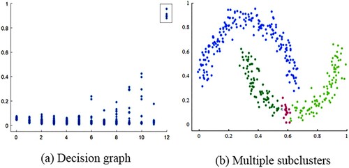
Figure 2. Decision graphs from different angles.

To automatically detect the cluster centres, a threshold-based method (Rodríguez & Laio, 2014) for finding out cluster centres is proposed, as shown in Equation (4), where $Threshol{d}_{\gamma }$ is chosen by users. (4) ${\gamma }_i={\rho }_i\times {\delta }_i>Threshol{d}_{\gamma }$(4) For any point $i$, if ${\gamma }_i>Thredrio{d}_{\gamma }$, it is considered as a cluster centre. Selecting the $Threshol{d}_{\gamma }$ is critical and will have a direct impact on the final clustering results. For a clearly distributed dataset, users can easily choose the value. But for complex datasets, choosing the ideal threshold is not an easy task. As shown in Figure 1(a), the points located in the upper right corner of the decision graph are concentrated, and it is difficult for the user to select the correct cluster centres. Then, there are multiple subclusters in the lower cluster, as shown in Figure 1(b).

2.2. Recent researches

Recently, some researchers have made a series of improvements in the automatic cluster centres detection problem. Liang and Chen (2016) introduced the idea of DBSCAN. They proposed a recursive partitioning strategy to find the correct number of clusters. Although this strategy obtained better results in automatic cluster centres detection of FDP, it still used the parameters of DBSCAN. There are also some works in which more sophisticated machine learning theories are used to detect cluster centres. Linear regression was used in the algorithm of Chen and He (2016) to select cluster centres. Jiang et al. (2019) came up with the idea of using gravity to improve the decision graph and made the density peaks easier to identify, but the identification process needed to be done manually. Because many problems can be regarded as optimisation problems (Liu et al., 2020), Other people transformed automatic cluster centres detection into optimisation problems. In Xu et al. (2020), the cluster centres were selected by optimising the Silhouette Coefficients. However, assigning clusters became iterative rather than being done in one step. Recently, Meng et al. (2020) used an adapted belief metric to make the cluster centres and outliers more salient. The approach still required manually selecting the cluster centres. Flores and Garza (2020) proposed a gap-based method for selecting cluster centres. Huang et al. (2016) used the percentiles of rho and delta to determine the cluster centres. We call the two algorithms DFDP and HFDP, respectively, and use them as comparison algorithms.

There are some related studies for the case of multiple subclusters in one cluster. Lin et al. (2020) used the neighbourhood radius to automatically select cluster centres and then applied single-chain clustering to reduce the cluster centres (DPSLC). But the method also needed the input of the correct number of clusters in advance. Wang et al. (2018) derived a new number similarity by introducing the definition of independence and affinity, which can better handle multiple density peaks in one cluster. But the method also required the input of the number of clusters. Wang et al. (2020) proposed based on a hierarchical method to merge clusters (McDPC). The data were classified with different density levels, and then the initial clustering was performed for each data point using the FDP method. Inspired by Liu et al. (2019), who applied directed weighted graphs to character merging, we think about whether weighted graphs can be used to merge subclusters. To use the FDP algorithm in large-scale datasets, Scholars have done many studies (Bai et al., 2017; Sieranoja & Fränti, 2019; Xu et al., 2018). Although FDP has been explored from several angles, there is still space for improvement, especially in scalability and preventing the algorithm from adding extra parameters.

An automated form of clustering algorithm is also needed in industrial production. In modern industrial production, people previously focused too much on the development of the control part. More important information has been neglected. Such as the behavioural characteristics of the operators involved, their experience, the state of the equipment and the production process. However, some machine learning algorithms can be a good solution to this problem. It can make full use of the accumulated historical and current data to extract potential patterns, rules and provide new perspectives for better industrial control.

3. The proposed algorithm

To solve the problems in the FDP algorithm, the A-FDP algorithm is improved in two aspects. On the one hand, a new $Threshol{d}_{\gamma }$ is designed to automatically select cluster centres. On the other hand, subcluster merging is completed by finding the connected components of the connected graph. In this section, the basic details of the A-FDP algorithm are given.

3.1. Automatic determination of cluster centres

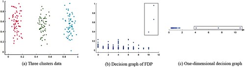
To find the proper $Threshol{d}_{\gamma }$, cluster centres (density peaks) can be referred to as outliers in the decision graph (Rodríguez & Laio, 2014). It means the cluster centres are clearly distinguished from other points in the decision graph. Figure 2(a) shows three clusters. The decision graph is obtained by using the FDP method, as shown in Figure 2(b). In this two-dimensional decision graph, it is clear the density peaks are the three points located in the upper right corner. To better observe the distribution of $\gamma$, we draw a one-dimensional decision graph in ascending order, as shown in Figure 2(c). We can find three points on the right side of the one-dimensional decision graph, which are far away from most of the points. Therefore, they can be regarded as outliers.

From the above description, we design a new automatic determination of cluster centres method by using outlier detection. A-FDP introduces Quartiles (Frigge et al., 1989) and the standard deviation to find cluster centres. Quartiles are arranged in statistics from the smallest to the largest and divided into quartiles at three split positions. The first quartile is the point at the 25% position, and the third quartile is the point at the 75% position. The difference between the third quartile and the first quartile is also called $IQR$ (InterQuartile Range). Besides, the standard deviation can reflect the dispersion of the data.

A-FDP uses Quartiles to describe $\gamma$. The quartile divides the ordered $\gamma$ into four parts, with each part containing a quarter of $\gamma$. Then, we consider both the $IQR$and the standard deviation to obtain the new threshold, which is defined as, (5) $Thredrio{d}_{\gamma }=1.5\times IQR+std(\gamma )$(5) where $std(\gamma )$ notes the standard deviation of $\gamma$. For any point $i$, if ${\gamma }_i>Thredrio{d}_{\gamma }$, it is considered as a cluster centre. In Frigge et al. (1989), anomaly detection is performed using 1.5 times $IQR$. In the present algorithm, 1.5 times $IQR$ is followed. After experiments, the new threshold can better detect the initial cluster centres, which will make the later subcluster merging process more efficient. About the choice of this value, we set a parameter $\alpha$ instead of 1.5, and the influence of this parameter will be discussed in Chapter 4.2.1.

Relying on the automatic cluster centres detection method, we can quickly obtain the cluster centres and initial clusters. However, this approach also results in multiple subclusters in a cluster due to inaccurate cluster centres reflected by the decision graph. For this case, the subcluster merging method is introduced to merge the initial clustering results.

3.2. Subcluster merging

Aiming at the case of multiple subclusters in a cluster, this section proposes a subcluster merging method. The basic idea is to construct a connected graph using the initial clustering centres chosen in the previous section. Subcluster merging is then performed by finding connected components on the connected graph. To express the subcluster merging method more clearly, some definitions are given as follows.

Definition 3.1

(Connected graph): In the undirected and weighted graph $G=(V,E)$, V represents the set of nodes composed of cluster centres, and E represents the edges between cluster centres. The weight of an edge is expressed as Connectivity.

Definition 3.2

(Connectivity): If the distance between points in two subclusters is less than $d_c$, then a micro-edge is added between the two nodes. The number of micro-edges is used as the Connectivity $C{d}_{l,m}$ of the two subclusters, as shown in Equation (6), where $S{C}_l$ and $S{C}_m$ represent different subclusters. (6) $C{d}_{l,m}=\left\{\text{number(}⟨i,j⟩)|i\in S{C}_l,j\in S{C}_m,d_{i,j}<d_c\right\}$(6)

Definition 3.3

(Cut edge): The connectivity of an edge is less than or equal to $\beta$ times the average Connectivity of all edges. The edge is called Cut edge $Ce(G)$, as shown in Equation (7), where $\frac{1}{2}$ is an adjustment parameter. After a lot of experiments, the parameter can be set from 0.2–0.7, and it is set to 0.5 in the experiment. (7) $Ce(G)\le \frac{1}{2}\times \overline{Cd}$(7)

When the distance of points between two clusters is larger than $d_c$, it means these two clusters are far away from each other. Correspondingly, the Connectivity of the edges of the two clusters is smaller. So, we need to remove edges when they satisfy the Cut edge condition.

When the distances between the points of any two subclusters are much greater than $d_c$, there is no edge between the nodes in the Connected graph, and then the subcluster merging process can be skipped at this time.

The specific subcluster merging idea is as follows. First, each cluster centre is considered as a node of the graph. The Connectivity between two nodes is used as the weight to obtain the Connected graph $G$. Second, the edges that satisfy the Cut edge condition need to be removed. Then, A-FDP finds all the connected components through a Depth-first search. Finally, all the subclusters corresponding to the nodes in the connected components are merged to get the new clustering result.

Figure 3(a) shows the Connected graph $G$. It can be known by calculating $C{d}_{1,3}$ and $C{d}_{1,4}$ are less than half of the average Connectivity of all edges and satisfy the condition of Cut edge. Therefore, the corresponding edge will be deleted. As shown in Figure 3(b), the algorithm finds the connected components of the last Connected graph. Finally, the subcluster represented by the corresponding nodes {2,3,4,5} will be merge. We will get the final clustering result ({1}, {2,3,4,5}).

Figure 3. Subcluster merging process.

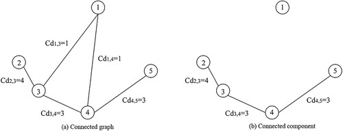
Figure 4. The selection of two parameters.

According to the above ideas, the steps of the A-FDP algorithm are described.

Table

Algorithm A-FDP

Input: The samples $X\in {\mathrm{\Re }}_{N\times M}$.

Output: The clustering result: $y\in {\mathrm{\Re }}_{N\times 1}$.

Step 1: Normalising the samples;

Step 2: calculate the distance matrix;

Step 3: Calculate ${\rho }_i$ and ${\sigma }_i$ according to Equations (2) and (3);

Step 4: Select the initial cluster centres according to Equations (4) and (5);

Step 5: assign remaining data to form the local cluster;

Step 6: Construct the Connected graph and calculate Connectivity degree and Cut edge according to Equations (6) and (7);

Step 7: Remove Cut edge, then get the connected component;

Step 8: Return y.

The time complexity of the A-FDP algorithm includes four aspects: (a)calculating the distance matrix, (b) calculating ${\rho }_i$ and ${\delta }_i$ of point $i$, (c) selecting the cluster centres, and (d) merging subcluster. The time complexity of these four parts is all $O(n^2)$. Therefore, the total time complexity of A-FDP is $O(n^2)$. The time complexity of A-FDP is the same as that of FDP, but it can get better clustering results.

4. Experiments and results analysis

4.1. Experimental settings

To verify the quality and accuracy of the A-FDP, the proposed A-FDP was tested and evaluated with two major classes of datasets, both the synthetic datasets and the UCI datasets (Dua & Graff, 2019)). Synthetic datasets Aggregation, Flame, and Spiral are obtained from the Clustering basic benchmark (Fränti & Sieranoja, 2018). The Moon dataset is a synthetic dataset. The details of the datasets in this paper are shown in Table 2, which includes the number of features, the number of samples, and the number of clusters for each dataset separately.

Table 2. The details of datasets.

Dataset		Features	Points	Clusters
Aggregation	synthetic	2	788	7
Flame		2	240	2
Spiral		2	312	3
Moon		2	800	2
Banknote	UCI	4	1372	2
Ecoli		8	336	8
Iris		4	150	3
Seeds		7	210	3
CMC		9	1473	3
Sonar		60	208	2

Before experimenting, we used the “min–max normalisation” method to process data. This way not only eliminates the impact of different dimensions on the experimental results but also reduces the running time of the algorithm.

The clustering results were compared with several clustering algorithms, including K-means (Jain, 2010), FCM (Fu, 1998), DBSCAN (Ester et al., 1996), FDP, AP (Frey & Dueck, 2007), DFDP, HFDP, DPSLC, and McDPC. These evaluations are Adjusted Rand Index (ARI) (Vinh et al., 2010), Normalized Mutual Information (NMI) (Strehl & Ghosh, 2002), and Adjusted Mutual Information (AMI) (Vinh et al., 2010). All three evaluation indicators are as close to 1 as possible.

About the unique parameter of K-means and FCM algorithms is the correct number of clusters, as shown in Table 2. For DBSCAN, two parameters need to be set: Eps and MinPts. We set MinPts=3, and Eps is selected from 0 to 0.5. The best results are chosen for each dataset. For DFDP, HFDP, FDP, DPSLC, and McDPC, the authors provide an empirical value of the number of neighbours that can be chosen $d_c$. We select the values of $d_c$ are from 1% to 2%. We adjust it to get the optimal result. A-FDP is selected the same way as FDP to set parameters $d_c$. AP algorithm only needs to be provided with one parameter, which is named Preference. The larger Preference, the more cluster centres are selected. We set the Preference as the median or min value of the similarity matrix according to the original author’s method. However, when the parameter Preference is set to the minimum value, the clustering obtains more clusters than the actual number of clusters. Therefore, in this experiment, the Preference is selected in a range smaller than the minimum value.

4.2. Experimental results and discussion

4.2.1. Experimental parameters selection

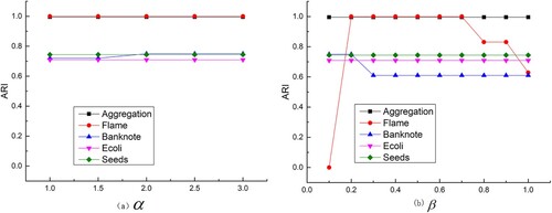
We set the value of $d_c$ to 2% of the total number of points. The effect of these two parameters on the performance of the A-FDP algorithm is evaluated. This experiment uses five datasets, including two synthetic datasets (Aggregation, Flame) and three UCI datasets (Banknote, Ecoli, Seeds). We use parameters $\alpha$ and $\beta$ instead of 1.5 and $\frac{1}{2}$, respectively. The clustering results for these five datasets at different values of $\alpha$ are shown in Figure 4(a). From this figure, we can clearly see that the parameter does not have a significant effect on the A-FDP. When parameter $\alpha$ is chosen to be 1.5, we choose different $\beta$ for the experiment and show it in Figure 4(b). It can be seen that when $\beta$ is chosen from 0.2 to 0.7, the performance of the A-FDP remains relatively stable and high.

The choice of cut-off distance $d_c$ affects the calculation of the local densities in equations (1) and (2), which in turn affects the overall clustering effect. We set the $d_c$ values from 1% to 2% of the distance to obtain the ARI values for the A-FDP algorithm at different $d_c$ values, as shown in Figure 5. We can see the A-FDP algorithm achieves more stable results when choosing from 1.5% to 2%. It can be seen the A-FDP algorithm has strong robustness, as long as the parameters are selected within the suitable range.

Figure 5. A-FDP experimental results under different $d_c$.

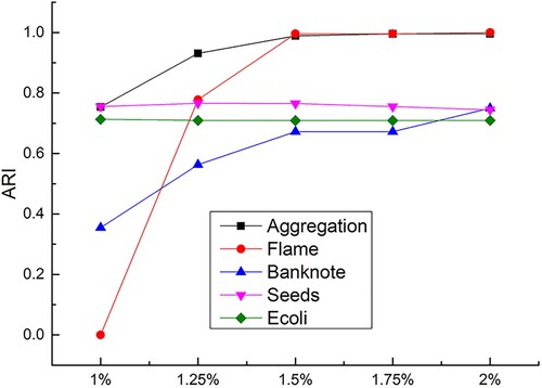
Figure 6. The process of A-FDP on the synthetic datasets.

4.2.2. Experimental on synthetic datasets and results analysis

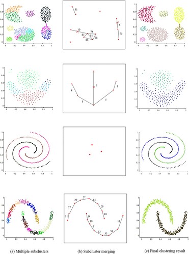
On the synthetic datasets, the A-FDP algorithm first uses Equation (5) to automatically select the cluster centres to get local clusters, as shown in Figure 6(a). The next step is subcluster merging, as shown in Figure 6(b). The red five-pointed star in Figure 6(b) represents the cluster centre selected by the one-dimensional decision graph, and the edges with a red “×” are Cut edges. Then, the final clustering results are obtained, as shown in Figure 6(c). But on some datasets, the distance between points of different subclusters is much larger than $d_c$. Then, the subcluster merging part will be skipped. The clustering results of the six clustering algorithms on the synthetic dataset are shown visually in Figures 7–10.

Figure 7. Clustering results on Aggregation.

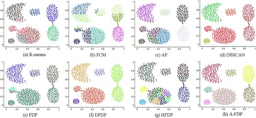
Figure 8. Clustering result on Flame.

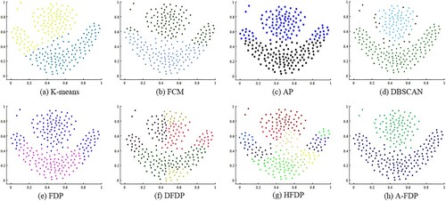
Figure 9. Clustering results on Spiral.

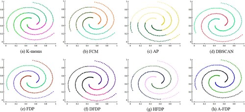
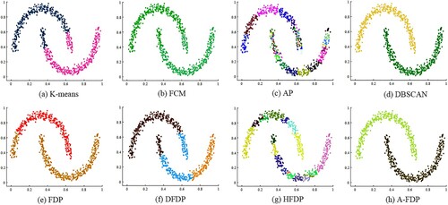
Figure 10. Clustering results on Moon.

As can be seen from Figure 7, the clustering result of A-FDP is the best on the Aggregation dataset. DBSCAN cannot separate two interconnected clusters despite finding all separated clusters. Multiple subclusters in a cluster occur in FDP and HFDP, which make clustering result poor as well. The clustering effect of FCM, K-means, AP, and DFDP is not good. These methods misclassify points in one cluster to another cluster.

In Figure 8, the K-means, FCM, AP, DFDP, and FDP algorithms do not perform well on the Flame dataset. DBSCAN considers some of the data points as noisy. HFDP wrongly divides a cluster into multiple subclusters. A-FDP algorithm has accurate results on the Flame dataset.

The Spiral dataset has a spiral shape rather than a spherical shape. Therefore, the K-means, FCM, and AP still have poor results on the Spiral dataset, as shown in Figure 9. The clustering results of DFDP and HFDP are not very good either. Conversely, the FDP, DBSCAN, and A-FDP algorithms perform well on the Spiral dataset.

In Figure 10, the Moon dataset is non-convex, which leads to unsatisfactory clustering results in K-means, FCM, and AP algorithms. DFDP, HFDP, and FDP methods still perform poorly on the Moon dataset. Because on the Moon dataset, there is more than one peak in one cluster. DBSCAN and A-FDP have satisfactory clustering results.

Table 3 shows the specific values of each of the three evaluations metrics on the different synthetic datasets. We can see in more detail the superiority of the A-FDP algorithm on the synthetic dataset. As can be seen from Table 3, the A-FDP algorithm performs the best, followed by the density-based DBSCAN algorithm. In contrast, the DFDP, HFDP, and FDP algorithms performed poorly. The relatively weak results of the K-means, FCM, and AP algorithms on these evaluation metrics are due to their inherent inefficiencies in clustering non-convex data.

Table 3. Comparison of ARI, NMI, and AMI on synthetic datasets.

	Aggregation			Flame			Spiral			Moon
Algorithm	ARI	NMI	AMI	ARI	NMI	AMI	ARI	NMI	AMI	ARI	NMI	AMI
A-FDP	0.996	0.992	1.000	1.000	1.000	1.000	1.000	1.000	1.000	1.000	1.000	1.000
FDP	0.881	0.892	0.997	0.336	0.392	0.381	1.000	1.000	1.000	0.663	0.637	0.629
DFDP	0.847	0.917	0.879	0.198	0.344	0.213	0.006	0.039	0.029	0.325	0.341	0.276
DFDP-1	0.891	/	/	0.950	/	/	1.000	/	/	/	/	/
HFDP	0.500	0.754	0.612	0.203	0.528	0.272	0.763	0.762	0.759	0.130	0.445	0.222
AP	0.684	0.826	0.778	0.487	0.442	0.428	−0.005	0.007	−0.005	0.099	0.359	0.358
DBSCAN	0.808	0.890	0.798	0.883	0.823	0.720	1.000	1.000	1.000	1.000	1.000	1.000
K-means	0.819	0.833	0.790	0.442	0.390	0.390	0.149	0.001	−0.005	0.521	0.419	0.418
FCM	0.589	0.738	0.693	0.487	0.442	0.428	−0.004	0.0015	−0.004	0.543	0.439	0.438

The above analysis shows that A-FDP is relatively better at the clustering of non-convex data and complex shape data than the K-means, FCM, AP, and FDP algorithms. Compared with DBSCAN, A-FDP does not have a complicated parameter adjustment process and does not produce more noise. The presence of multiple subclusters in a cluster is a significant improvement compared to DFDP and HFDP. To further demonstrate the performance of the A-FDP, in the following subsections, the clustering results on UCI datasets will be shown.

4.2.3. Experimental on UCI datasets and results analysis

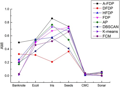
Six UCI datasets are selected for this set of experiments, and the clustering results of A-FDP are compared with the DFDP, HFDP, FDP, AP, DBSCAN, K-means, and FCM algorithms, as shown in Figures 11–13. The clustering results of A-FDP on ARI, NMI, and AMI are shown, respectively. We can see that all the algorithms do not perform very well on the high-dimensional datasets CMC and Sonar, but the A-FDP algorithm has a slight advantage in clustering results. Due to the diversity of the different datasets, no one clustering algorithm was better than the others on six datasets. Mostly, A-FDP has the best clustering results, which suggests that A-FDP can handle datasets with different internal structures.

Figure 11. Comparison of ARI on UCI datasets.

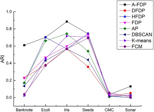
Figure 12. Comparison of NMI on UCI datasets.

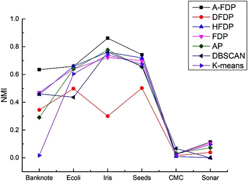
Figure 13. Comparison of AMI on UCI datasets.

As shown in Table 4, the A-FDP algorithm performs better compared to the DPSLC, McDPC algorithm which has merged subclusters.

Table 4. Comparison of ARI for DPSLC, McDPC, A-FDP algorithms.

Algorithm	Aggregation	Flame	Spiral	Moon	Banknote	Ecoli	Iris	Seeds	CMC	Sonar
DPSLC	0.996	0.988	1	/	/	/	/	/	/	/
McDPC	1	0.013	0.932	/	/	0.9	0.890	0.700	/	0
A-FDP	0.996	1	1	1	0.371	0.702	0.890	0.777	0.04	0.13

In general, the A-FDP is highly robust when the parameters are set in the right range. A-FDP can also obtain high-quality clustering results regardless of spherical and non-spherical data, small and large data. A-FDP generally outperforms the DFDP, HFDP, FDP, DBSCAN, K-means, FCM, and AP algorithms in three clustering performance evaluation metrics. For synthetic datasets, the three performance indicators of A-FDP are the best, which shows that A-FDP has superior performance on two-dimensional datasets. A-FDP still has better clustering results on most UCI datasets compared with other clustering algorithms.

5. Conclusion

In this paper, we propose a new automatic clustering method (A-FDP) to improve the FDP algorithm. A-FDP solves manually selecting cluster centres in FDP through the newly designed method of automatically selecting cluster centres. A-FDP uses Quartiles to describe the multiple $\gamma$ of local density $\rho$ and high density nearest distance $\delta$ and finds the difference between the third quartile and the first quartile as the InterQuartile Range. Then, a new decision threshold is designed in A-FDP combined with the InterQuartile Range and standard deviation. We select the points larger than the decision threshold as the cluster centres. Besides, A-FDP uses the idea of finding connected components to merge subclusters, which improves the case of multiple subclusters in a cluster. The experimental results show that, especially for FDP, compared with other classic clustering algorithms, the A-FDP algorithm gains better clustering results. For the FDP algorithm, we can also improve the distance calculation to make it more suitable for more complex datasets. Alternatively, we can challenge adaptive selection methods that optimise cut-off distances, which can be used to solve clustering problems on data with different densities. In recent years, more and more data has been presented dynamically. So, we can study new clustering algorithms to apply to streaming data.

Disclosure statement

No potential conflict of interest was reported by the author(s).

Additional information

Funding

This work was supported by the National Natural Science Foundation of China [grant number 619 62054].

References

- Bai, L., Cheng, X., Liang, J., Shen, H., & Guo, Y. (2017). Fast density clustering strategies based on the k-means algorithm. Pattern Recognition, 71, 375–386. https://doi.org/10.1016/j.patcog.2017.06.023.
- Chen, J., & He, H. (2016). A fast density-based data stream clustering algorithm with cluster centers self-determined for mixed data. Information Sciences, 345, 271–293. https://doi.org/10.1016/j.ins.2016.01.071.
- Cheung, Y. M. (2005). Maximum weighted likelihood via rival penalized EM for density mixture clustering with automatic model selection. IEEE Transactions on Knowledge and Data Engineering, 17(6), 750–761. https://doi.org/10.1109/TKDE.2005.97.
- Dua, D., & Graff, C. (2019).UCI machine learning repository.
- Ester, M., Kriegel, H.-P., Sander, J., & Xu, X. (1996). A density-based algorithm for discovering clusters in large spatial databases with noise .. Proceedings of the Second International Conference on Knowledge Discovery and Data Mining, Portland, Oregon, USA.
- Fahad, A., Alshatri, N., Tari, Z., Alamri, A., Khalil, I., Zomaya, A., Foufou, S., & Bouras, A. (2014). A survey of clustering algorithms for big data: Taxonomy and empirical analysis. IEEE Transactions on Emerging Topics in Computing, 2(3), 267–279. https://doi.org/10.1109/TETC.2014.2330519.
- Flores, K. G., & Garza, S. E. (2020). Density peaks clustering with gap-based automatic center detection. Knowledge-Based Systems, 206, 106350. https://doi.org/10.1016/j.knosys.2020.106350.
- Fränti, P., & Sieranoja, S. (2018). K-means properties on six clustering benchmark datasets. Applied Intelligence, 48(12), 4743–4759. https://doi.org/10.1007/s10489-018-1238-7.
- Frey, B., & Dueck, D. (2007). Clustering by passing messages between data points. Science, 315(5814), 972–976. https://doi.org/10.1126/science.1136800.
- Frigge, M., Hoaglin, D. C., & Iglewicz, B. (1989). Some implementations of the boxplot. The American Statistician, 43(1), 50–54. https://doi.org/10.1080/00031305.1989.10475612.
- Fu, G. (1998). Optimization methods for fuzzy clustering. Fuzzy Sets and Systems, 93(3), 301–309. https://doi.org/10.1016/S0165-0114(96)00227-8.
- Guo, G., Zhang, J., & Yorke-Smith, N. (2015). Leveraging multiviews of trust and similarity to enhance clustering-based recommender systems. Knowledge-Based Systems, 74, 14–27. https://doi.org/10.1016/j.knosys.2014.10.016.
- Havens, T. C., Bezdek, J. C., Leckie, C., Hall, L. O., & Palaniswami, M. (2012). Fuzzy c-means algorithms for very large data. IEEE Transactions on Fuzzy Systems, 20(6), 1130–1146. https://doi.org/10.1109/TFUZZ.2012.2201485.
- Huang, L., Wang, G., Wang, Y., Pang, W., & Ma, Q. (2016). A link density clustering algorithm based on automatically selecting density peaks for overlapping community detection. International Journal of Modern Physics B, 30(24), 1650167. https://doi.org/10.1142/S0217979216501678.
- Jain, A. (2010). Data clustering: 50 years beyond K-means. Pattern Recognition Letters, 31(8), 651–666. https://doi.org/10.1016/j.patrec.2009.09.011.
- Jiang, J., Chen, J., Meng, X., Wang, L., & Li, K. (2019). A novel density peaks clustering algorithm based on k nearest neighbors for improving assignment process. Physica A: Statistical Mechanics and its Applications, 523, 702–713. https://doi.org/10.1016/j.physa.2019.03.012.
- Law, L. T., & Cheung, Y. M. (2003). Color image segmentation using rival penalized controlled competitive learning. Proceedings of the International Joint Conference on Neural Networks, 1, 108–112. https://doi.org/10.1109/IJCNN.2003.1223306
- Liang, Z., & Chen, P. (2016). Delta-density based clustering with a divide-and-conquer strategy: 3DC clustering. Pattern Recognition Letters, 73, 52–59. https://doi.org/10.1016/j.patrec.2016.01.009.
- Lin, J., Kuo, J., & Chuang, H. (2020). Improving density peak clustering by automatic peak selection and single linkage clustering. Symmetry, 12(7), 1168. https://doi.org/10.3390/sym12071168.
- Liu, H., Wang, Y., & Fan, N. (2020). A hybrid deep grouping algorithm for large scale global optimization. IEEE Transactions on Evolutionary Computation, 24(6), 1112–1124. https://doi.org/10.1109/TEVC.2020.2985672.
- Liu, S., Wang, Y., Tong, W., & Wei, S. (2019). A fast and memory efficient MLCS algorithm by character merging for DNA sequences alignment. Bioinformatics, 36(4), 1066–1073. https://doi.org/10.1093/bioinformatics/btz725.
- Lu, J., Tan, Y., Wang, G., & Yang, G. (2013). Image-to-set face recognition using locality repulsion projections and sparse reconstruction-based similarity measure. IEEE Transactions on Circuits and Systems for Video Technology, 23(6), 1070–1080. https://doi.org/10.1109/TCSVT.2013.2241353.
- Meng, J., Fu, D., & Tang, Y. (2020). Belief-peaks clustering based on fuzzy label propagation. Applied Intelligence, 50(4), 1259–1271. https://doi.org/10.1007/s10489-019-01576-4.
- Nilashi, M., Bagherifard, K., Rahmani, M., & Rafe, V. (2017). A recommender system for tourism industry using cluster ensemble and prediction machine learning techniques. Computers & Industrial Engineering, 109, 357–368. https://doi.org/10.1016/j.cie.2017.05.016.
- Qian, J., Zhao, R., Wei, J., Luo, X., & Xue, Y. (2020). Feature extraction method based on point pair hierarchical clustering. Connection Science, 32(3), 223–238. https://doi.org/10.1080/09540091.2019.1674246.
- Ren, Y. J., Shen, J., Wang, J., Han, J., & Lee, S. Y. (2015). Mutual verifiable provable data auditing in public cloud storage. Journal of Internet Technology, 16(2), 317–323. https://doi.org/10.6138/JIT.2015.16.2.20140918.
- Rodríguez, A., & Laio, A. (2014). Clustering by fast search and find of density peaks. Science, 344(6191), 1492–1496. https://doi.org/10.1126/science.1242072.
- Sieranoja, S., & Fränti, P. (2019). Fast and general density peaks clustering. Pattern Recognition Letters, 128, 551–558. https://doi.org/10.1016/j.patrec.2019.10.019.
- Strehl, A., & Ghosh, J. (2002). Cluster ensembles: A knowledge reuse framework for combining multiple partitions. Journal of Machine Learning Research, 3, 583–617. https://doi.org/10.1002/widm.32 .
- Tourinho, I., & Rios, T. (2021). FACF: Fuzzy areas-based collaborative filtering for point-of-interest recommendation. International Journal of Computational Science and Engineering, 24(1), 27–41. https://doi.org/10.1504/IJCSE.2021.113636.
- Vinh, N. X., Epps, J., & Bailey, J. (2010). Information theoretic measures for clusterings comparison: Variants, properties, normalization and correction for chance. Journal of Machine Learning Research, 11, 2837–2854. https://doi.org/10.1145/1553374.1553511.
- Wang, C., Zhao, T., & Mo, X. (2019). The extraction of security situation in heterogeneous log based on Str-FSFDP density peak cluster. International Journal of Computational Science and Engineering, 20(2), 387–396. https://doi.org/10.1504/IJCSE.2019.103943.
- Wang, G., Wei, Y., & Tse, P. (2018). Clustering by defining and merging candidates of cluster centers via independence and affinity. Neurocomputing, 315, 486–495. https://doi.org/10.1016/j.neucom.2018.07.043.
- Wang, Y., Wang, D., Zhang, X., Pang, W., Miao, C., Tan, A. H., & Zhou, Y. (2020). McDPC: Multi-center density peak clustering. Neural Computing and Applications, 32(17), 13465–13478. https://doi.org/10.1007/s00521-020-04754-5.
- Wu, Y., Peng, X., Mohammad, N., & Yang, H. (2021). Research on fuzzy clustering method for working status of mineral flotation process. International Journal of Embedded Systems, 14(2), 133–142. https://doi.org/10.1504/IJES.2021.113805.
- Xia, Z., Wang, X., Zhang, L., Qin, Z., Sun, X., & Ren, K. (2016). A privacy-preserving and copy-deterrence content-based image retrieval scheme in cloud computing. IEEE Transactions on Information Forensics and Security, 11(11), 2594–2608. https://doi.org/10.1109/TIFS.2016.2590944.
- Xu, X., Ding, S., & Shi, Z. (2018). An improved density peaks clustering algorithm with fast finding cluster centers. Knowledge-based Systems, 158, 65–74. https://doi.org/10.1016/j.knosys.2018.05.034.
- Xu, X., Ding, S., Wang, L., & Wang, Y. (2020). A robust density peaks clustering algorithm with density-sensitive similarity. Knowledge-Based Systems, 200, 106028. https://doi.org/10.1016/j.knosys.2020.106028.
- Zhao, F., Liu, H., & Fan, J. (2015). A multi objective spatial fuzzy clustering algorithm for image segmentation. Applied Soft Computing, 30, 48–57. https://doi.org/10.1016/j.asoc.2015.01.039.
- Zhao, Q., Li, X., Li, Y., & Zhao, X. (2017). A fuzzy clustering image segmentation algorithm based on hidden Markov random field models and Voronoi tessellation. Pattern Recognition Letters, 85, 49–55. https://doi.org/10.1016/j.patrec.2016.11.019.