An efficient sparse pruning method for human pose estimation

Abstract

Human pose estimation (HPE) is crucial for computer vision (CV). Moreover, it’s a vital step for computers to understand human actions and behaviours. However, the huge number of parameters and calculations in the HPE model have brought big challenges to deploy to resource-constrained mobile devices. Aiming to overcome the challenge, we propose a sparse pruning method (SPM) for the HPE model. First, L1 regularisation is added in the training phase of the original model, and network parameters of the convolution layers (CLs) and batch normalisation layers (BNLs) are sparsely trained to obtain a network structure with sparse weights. We then combine the sparse weights of filters with the scaling parameters of the BNLs to determine their importance. Finally, the structured pruning method is used to prune the sparse filters and corresponding channels. SPM can reduce the number of model parameters and calculations without affecting precision. Promising results indicate that SPM outperforms other advanced pruning methods.

KEYWORDS:

• Human pose estimation
• computer vision
• sparse pruning method
• scaling parameters
• structured pruning method

1. Introduction

At present, computer vision is still one of the most attractive deep learning research disciplines, which mainly includes the following four tasks: image classification (Ying et al., 2021), object detection (Srivastava & Biswas, 2020; Sun et al., 2021), semantic segmentation (Jiang et al., 2021; Wu et al., 2019), and instance segmentation (Xu & Zhang, 2020). HPE has attracted considerable attention in CV. It is a technique for anticipating key points on the human body, as well as a crucial step in comprehending human behaviour. HPE is progressively being used in numerous parts of daily life, thanks to the rapid growth of the field. To complete character special effects, for example, HPE can be applied to a computer graphic image utilising motion capture and augmented reality. HPE can also be used to track the movement of human objects to achieve human–computer interaction (Doshi-Velez & Roy, 2008; Li et al., 2019, 2020; Ning, Duan, et al., 2020; Ning, Nan, et al., 2020; Suzuki & Katagiri, 2007; Zhang, Li, et al., 2021; Zhang, Sun, et al., 2021)n pose estimation technology shines in the fields of security monitoring and behaviour recognition (Bianchi-Berthouze & Kleinsmith, 2003; Ning, Gong, Li, and Zhang, 2021; Ning, Gong, Li, Zhang, Bai, et al., 2021; Yan et al., 2020). New HPE approaches, such as DeepPose (Toshev & Szegedy, 2014), OpenPose (Cao et al., 2019), convolutional pose machine (Wei et al., 2016), stacked hourglass (Newell et al., 2016), high-resolution network (HRNet) (Sun et al., 2019), have been developed recently as deep learning and convolutional neural networks (CNNs) have advanced. Existing human pose estimation approaches often focus on ways to increase the model’s generalisation performance and pose estimate precision, while disregarding key efficiency issues. Furthermore, the enormous number of parameters and calculations in the model have led to big challenges to the deployment of resource-constrained mobile devices. Therefore, model compression has emerged as one of academia’s and industry’s most significant study areas.

Lightweight network design has recently been studied to increase the efficiency of posture estimation networks. Bulat and Tzimiropoulos (2017) applied neural network binarisation to the pose estimation network to achieve model compression, which is suitable for applications with limited computational resources, but with significantly reduced performance. Zhang et al. (2019) introduced a lightweight network for HPE, that can achieve high-speed inference on non-GPU platforms, but with a large loss of recognition precision. The core idea of these previous lightweight methods is to achieve model compression by designing a lightweight network structure. Although the network has advantages in model size and computational complexity, it also loses high precision. The purpose is to compress the model on the basis of ensuring the high precision of the pose estimation as much as possible, so we focus our work on designing an efficient model pruning method rather than designing a lightweight pose estimation network.

Model pruning is a strategy for reducing the number of model parameters and calculations while also accelerating and compressing the model. LeCun et al. (1989) suggested a pruning strategy for neural networks called optimal brain damage (OBD). OBD decreases the number of model parameters while simultaneously improving the model’s generalisation performance by removing unimportant weights from the network. Li et al. (2017) used the L1-Norm of each layer of the network to determine its importance and removed unimportant filters of the network and their feature maps, thereby greatly reducing the computational cost. In total, the key to model pruning is how to determine the importance of the network structure. This importance is expressed by factors such as weights (Li et al., 2017), channel entropy (Luo & Wu, 2017), and scaling factor (Liu et al., 2017).

The sparse model has recently played an increasingly crucial role in the field of model compression. First, it can solve the problem of overfitting in modelling through the function of variable selection. Second, redundant variables in the model can be deleted after sparseness, and only explanatory variables having the greatest correlation with the response variable are retained, so that the model parameters are sparse, and a sparse network model is obtained. Finally, the sparse model has better interpretability and reduces the number of model calculations required.

In the model pruning work, after using weights pruning or filters pruning alone, the complexity of the model obtained remains very high. In this article, we propose SPM for solving the aforementioned problems and for facilitating the deployment of resource-constrained devices. By combining the sparsity of the CL with the BNL, we may train the model sparsely and prune unimportant filters, resulting in a sparse network structure. Unlike many other approaches, the proposed importance determination function uses two-layer network information of the CL and the BNL to improve importance determination accuracy. Furthermore, our strategy significantly decreases the model’s training cost and size, and the model requires no special libraries/hardware to deploy on mobile devices. The following are our contributions:

• We propose SPM for HPE, which can compress and accelerate the model while ensuring precision and facilitating deployment on mobile devices.

• We establish a novel loss function, $\text{Los}{\text{s}}^{\ast }$, that adds L1 regularisation to the weights of the CLs and the scaling parameters of the BNLs on the basis of the original loss function to promote the weight of lower importance and the scaling factor to approach 0 to achieve sparseness.

• We introduce a simple and efficient metric, $I_j$, to evaluate the importance of filters. Compared with the scaling factor based metric (Liu et al., 2017), our metric combines the two-layer network information of the CL and BNL to enhance the accuracy of importance determination.

• Experiments on different datasets demonstrate that SPM can decrease the number of model parameters and calculations in the HRNet model by 40% to 70% while maintaining precision comparable to the original model. In addition, because the pruned model does not have any sparse storage format or computational operations, our strategy improves model compression and inference time with traditional deep learning hardware and software packages.

2. Related work

2.1. Human pose estimation

The pictorial structural model or the probabilistic graphical model are used in the majority of classic HPE algorithms (Pishchulin et al., 2013; Yang & Ramanan, 2011). CNNs now provide dominant solutions for HPE, due to the introduction of DeepPose (Toshev & Szegedy, 2014). There are two common approaches: directly regressing keypoint coordinates (Toshev & Szegedy, 2014) and generating keypoint heatmaps followed by choosing the index corresponding to the peak as the keypoints (Cao et al., 2019; Newell et al., 2016; Sun et al., 2019; Wei et al., 2016).

The application of deep neural networks (DNNs) has accelerated development in the field of HPE recently. To improve HPE performance, Wei et al. (2016) introduced CPM for the task of HPE and employed a sequential convolution structure model to learn to express spatial information. Newell et al. (2016) presented a stacked hourglass network for the task of HPE, which processes and merges the information features of all scales of the image to better capture the numerous spatial connections associated to the body. Cao et al. (2019) proposed OpenPose using part affinity fields (PAFs), which ranked first in the inaugural COCO 2016 keypoints challenge. Sun et al. (2019) presented HRNet for HPE achieved better performance, which can generate accurate and spatially accurate keypoint heatmaps.

In these previous works, HRNet has superior performance compared to other HPE models. It is a very representative and universal network in the field of HPE. However, its complex structure and high computational cost make it extremely difficult to deploy and apply on edge devices. So this paper pays more attention to how to prune the HRNet model under the premise of ensuring its precision.

2.2. Model pruning methods

Model pruning is a mainstream method for effectively implementing model compression, which can obtain a network model with a few parameters and calculations by pruning low-importance neurons, filters, or channels in the network. Han et al. (2015) set the weights of the model lower than the preset threshold to zero to prune the neurons when training the initial model. On the basis of the findings of Han et al. (2015), Guo et al. (2016) improved the neuron pruning method and proposed a dynamic network pruning strategy. This strategy can continuously restore important connections that were incorrectly pruned during pruning and improve network precision.

However, the neuron pruning method is unstructured and can only be accelerated through specialised sparse matrix libraries and specific hardware. Structural pruning (Guo et al., 2020; He et al., 2017, 2018; Lin et al., 2020; Liu et al., 2017; You et al., 2019; Zhuang et al., 2018) compensates for the disadvantage of unstructured pruning and enables the model to be deployed directly to a common device platform. He et al. (2017) presented a new channel pruning approach on basis of lasso regression and least-squares reconstruction to accelerate the DNNs with minimal precision loss. Zhuang et al. (2018) suggested a discrimination-aware channel pruning strategy that incorporated extra losses into the network throughout the fine-tuning and pruning phases to strengthen the discriminative power of intermediate layers and improve the channel feature recognition capacity after pruning. Some methods (Guo et al., 2020; He et al., 2018; Lin et al., 2020; You et al., 2019) belong to filter-level pruning. Because the original convolution structure is retained after pruning, there is no need to rely on specialised hardware/libraries. The pruning method proposed in this paper is to use structural pruning for model compression.

Regardless of whether structured or unstructured model pruning is used, the importance of model parameters needs to be determined first. Li et al. (2017) set the weight of network parameters as the criterion of their importance, pruning the network parameters below a specific threshold. Luo and Wu (2017) considered the convolution kernel with a smaller entropy value to be less important, and then pruned the convolution kernel with a smaller entropy value. Liu et al. (2017) choose the scaling parameter in the BNL as the channel importance indicator to determine which channel is unimportant and can be removed. The importance judgment of the aforementioned method is only based on the information of the network parameters themselves, and the single-layer information will affect the accuracy of the importance judgment. The importance judgment function proposed in this paper combines the two-layer network information of the CL and BNL to enhance the accuracy of importance judgment.

2.3. Sparse methods

With the development of research, many scholars have used various sparsity methods to make the model structure sparse. The precision of the original model can be maintained on the basis of a higher compression ratio. Changpinyo et al. (2017) presented a sparse strategy for sparse operation of the deep convolution network, which enhances the model’s generalisation performance and effectively compresses the model. Wen et al. (2016) offered a structured sparsity learning (SSL) strategy for forcing DNNs to learn more concise architectures while maintaining precision. Through existing libraries, the compact DNN structure could greatly enhance model inference speed on the CPU and GPU, making it easier to deploy on resource-constrained mobile devices.

3. Model and method

3.1. Model

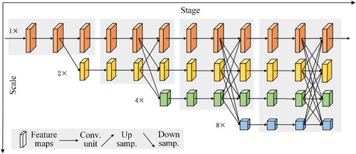
HRNet (Sun et al., 2019) is divided into three sections: basic block, bottleneck, and multi-scale fusion layer. Specifically, HRNet contains four phases, starting with the high-resolution subnet, then adding high-to-low resolution subnets one after another, and connecting the multi-resolution subnets in parallel. In short, the resolutions of the parallel subnet in the next phase include the high resolutions of the previous phase and a lower resolution. HRNet adopts a multi-scale fusion method to enhance the high-resolution representation of the network which generates a more accurate prediction of the key point heat map, improving the precision of HPE consequently. As shown in Figure 1, the horizontal direction represents the stage of the HRNet and the vertical direction corresponds to the scale of the feature maps. The resolution of the four parallel subnets in HRNet is gradually halved and the number of channels is doubled. The 1st phase comprises 4 residual units and then the width of the feature map is reduced by one 3 × 3 convolution. The next three phases, respectively, include 1, 4, and 3 exchange blocks. There are 4 residual units in an exchange block. Each residual unit in an exchange block includes two 3 × 3 convolutions and an exchange unit across resolutions. HRNet is difficult to deploy to mobile devices because of its complex network structure. Therefore, we considered it as the object of model pruning.

Figure 1. Architecture of HRNet.

3.2. Method

To effectively compress and accelerate HRNet, a new pruning method called SPM is presented in the paper. The sparse pruning scheme based on HRNet is shown in Figure 2. For the original HRNet model, we first used L1 regularisation to sparsely train its network parameters, pruned the sparsely trained model structurally, deleted the filters and with low importance, and finally restored the performance of the pruned model through model retraining. Below, we introduce our proposed method in detail.

Figure 2. Flowchart of the sparse pruning scheme.

3.2.1. Sparse training

The purpose of model sparse training is to make some parameters in the dense weight matrix tend to 0 or equal to 0, so that the model structure with sparse weights can be obtained. By combining the weight information of the CL and BNL, the importance of corresponding filters or channels can be determined and pruned, which reduces the cost of model operation and achieves the purpose of model compression and acceleration. HRNet contains numerous CLs and BNLs. For CLs, we can achieve model compression and acceleration by deleting some filters. The BNL is generally located after the CL. Its function is to normalise the output of the upper CL to accelerate the convergence of networks. Specifically, the operation process of the BNL is given by (1) $y_i=\gamma \frac{x_i-{\mu }_B}{\sqrt{{\sigma }_B^2+}ϵ}+\beta$(1) where $x_i$ is the input of the BNL and $y_i$ is the output of the BNL, ${\mu }_B$ and ${\sigma }_B^2$ are the mean and variance values of input activations, ε is a constant that can be introduced to the variance to enhance numerical stability, and $\gamma$ and $\beta$ are the scaling factor and offset factor of the corresponding active channel, respectively (Ioffe & Szegedy, 2015). The scaling factor of each BNL corresponds to each active channel, and we can determine the redundant active channel by scaling factor. Because each active channel is obtained by convolution operation of the corresponding filter in the upper CL, the scaling factor can indirectly reflect the importance of the filter in the corresponding CL.

In sparse training, we added L1 regularisation to the CL weights and the scaling parameter of the BNL, and trained and updated the weight and scaling factor to make the weight and scaling factor of lower importance approach 0 to achieve sparseness. At the same time, the regularisation factor was introduced to restrict the CL weights and the scaling parameter of the BNL, so the loss function is given by (2) ${Loss}^{\ast }=Loss+\lambda (L_1(W)+L_1(\gamma ))$(2) where $Loss=\sum _{(x,y)}L(f(x,W),y)$ represents the original loss function, $x$ represents the train input and $y$ is the train target, $W=\{W_1,W_2,\dots ,W_L\}$ represents the weights set of all CLs, $\gamma =\{{\gamma }_1,{\gamma }_2,\dots ,{\gamma }_L\}$ represents the scaling factors set of all BNLs, $\lambda$ is the regularisation factor for controlling the degree of sparse training, and $L_1(\cdot )$ represents L1 regularisation. For CL weights, $L_1(W)\sum _{l=1}^L\Vert W_l\Vert$. For the scaling factor $\gamma$, $L_1(\gamma )=\sum _{L=1}^L{\Vert {\gamma }_l\Vert }_1$.

3.2.2. Pruning and retraining

Model pruning is to prune the less important filters or channels after model sparse training. In this study, the importance of the filter or channel was determined using the weight information of the convolution filter and the corresponding scaling parameter of the BNL. So, the importance determining function $I_j$ is described as (3) $I_j=F_j\times {\gamma }_j$(3) where $I_j$ represents the importance score of the jth filter, $F_j$ is the sum of the absolute weights of the jth filter, and $F_j={\sum }_{i=1}^m|w_i|$, ${\gamma }_j$ represents the scaling factor of the corresponding BNL of the jth filter.

When pruning the channels of the sparsely trained model, we need to determine the global pruning threshold of the model. Refer to equation (4), we can get the set of importance scores $I=\{I_1,I_2,\dots ,I_n\}$ for all filters in the model. Assuming that the pruning rate of the model is $P$, then the pruning threshold $I^{\ast }$ is calculated refer to (4) $I^{\ast }=\text{sor}{\text{t}}_P(I)$(4) where the function $\text{sor}{\text{t}}_P(I)$ sorts the importance scores in an ascending order and outputs the value at $P$.

The multi-scale fusion layer in HRNet contains more information and fewer network parameters; therefore, it does not participate in the model pruning process. At the same time, because both basic block and bottleneck in the model have structures similar to the residual network (He et al., 2016), the convolution operation before the “add” operation involves multi-scale fusion, so the convolution operation does not participate in model pruning. As shown in Figure 3, the structure enclosed in the dotted rectangle box is the pruning area. Regarding the sparse pruning of the HRNet model, as shown in Figure 4, pruning the filter or channel whose importance score is below the set threshold leads to deletion of the output feature graph, and the HRNet model with a simplified structure is obtained. When the pruning rate is high, the precision of HPE may decrease as a result. However, the subsequent retraining process can restore the precision of the pruned network to a large extent.

Figure 3. The HRNet network structure pruning area. (a) The basic block architecture and (b) the bottleneck architecture. The structure enclosed in the dotted rectangle box is the pruning area.

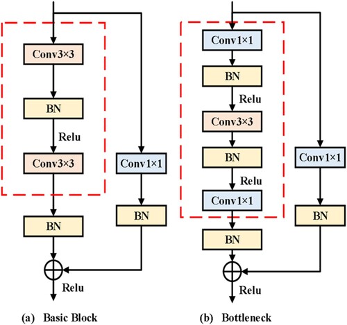
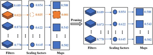
Figure 4. We associate the scaling parameter of the BNL with the corresponding filter of the upper CL. During the training process, L1 regularisation is applied to filter weights and scale factors to automatically select filters with low importance. The filters with a small importance score will be pruned. After pruning, we get the simplified model, which is then retrained to match the original model precision.

4. Experiments

The datasets and evaluation metric utilised in the experiment, as well as, the detailed design of the experiment, are described in this section.

4.1. Datasets and evaluation criteria

To compare the results of model pruning on various datasets, the COCO dataset (Lin et al., 2014) and MPII Human Pose dataset (Andriluka et al., 2014) were selected as experimental datasets. The COCO dataset, which includes around 200,000 pictures and 250,000 person samples with 17 keypoint labels, is a typical dataset for human keypoint detection. There are 57 K pictures and 150 K person samples in the COCO train2017 dataset. There are also 5 and 20 K photos in the val2017 and test-dev2017 datasets, correspondingly. The MPII Human Pose dataset comprises approximately 25 K photos from daily human activities, including more than 40 K annotated human joints, 12 K human goals in the test set, and the rest for training.

The standard evaluation metric for HRNet tested on the COCO dataset is on the basis of object keypoint similarity (OKS): (5) $\text{OKS}=\frac{{\sum }_i\text{exp}(-d_i^2/2s^2{k}_i^2)\delta (v_i>0)}{{\sum }_i\delta (v_i>0)}$(5) where $d_i$ denotes the Euclidean distance between the estimated keypoint and the corresponding ground truth value, $s$ represents object scale, $k_i$ represents the factor of keypoint that determines attenuation, $v_i$ indicates the visible mark of the ground truth value. The evaluation metrics used in this study were average precision (AP scores at OKS = 0.50, 0.55, … , 0.95) and average recall scores (AR scores at OKS = 0.50, 0.55, … , 0.95). The standard evaluation metric for HRNet tested on the MPII is the [email protected](α = 0.5) score (Sun et al., 2019).

4.2. Datasets and evaluation metric

Three models with distinct structures are chosen in this paper to evaluate the approach on COCO and MPII datasets: HRNet-W32-384 × 288, HRNet-W32-256 × 256, and HRNet-W48-384 × 288 where 32 and 48 denote the number of channels of the high-resolution subnets in the final three phases. In addition, 256 × 256 and 384 × 288 indicate the size of the input images. The initial models utilised on the COCO dataset are the small model HRNet-W32-384 × 288 and the big model HRNet-W48-384 × 288. The purpose is to test the general applicability in small and big models. HRNet-W32-256256 are used on the MPII dataset for a fairer comparison.

Adam Optimiser (Kingma & Ba, 2015) was adopted in the experiment during the model training stage. We trained 210 epochs on the COCO and MPII datasets with a specific learning rate of 10⁻³, then decreased it to 10⁻⁴ and 10⁻⁵ at the 170th and 200th epochs. The regularisation parameter of 10⁻⁵ is used to train the original model sparsely. When pruning the filters of a sparsely trained model, we first need to determine the pruning threshold of the model. The pruning threshold was determined by the percentage of all importance scores, such as pruning 40% or 80% filters. The purpose of pruning is to delete several filters from the sparse trained model to form a simple model. Finally, the precision of the model was restored by retraining the pruned model. The optimisation settings utilised in the retraining are the same as in the sparse training.

5. Results and analysis

We completed enough tests to prove that our pruning strategy is effective in HPE. In this part, we provide the main experimental findings and analysis. We herein discuss the effects of regularisation parameters on sparse training and the effects of different pruning rates on model precision. In addition, we compare the pruning methods proposed in this paper with other pruning schemes and prove the superiority of our pruning methods.

5.1. Results on COCO and MPII

The results on two datasets are shown in Tables 1 and 2. “Baseline” denotes normal training without sparsity regularisation. “40% pruned” means the model with 40% filters pruned from the sparsely trained model. Params are parameters that correspond to the amount of memory that the model takes up and directly represent the effect of model compression. GFLOPs are operations that correspond to the floating-point operations per second of the model, which can help illustrate the effect of model acceleration. We list the best results in bold. A comparison of the evaluation metrics before and after pruning shows that the Params and GFLOPs of the model are obviously compressed after pruning, while the precision of the model is almost unaltered. This demonstrates the validity of the pruning strategy used in this study. Tables 1 and 2 show that the parameters and GFLOPs of the small models HRNet-W32-384 × 288 and HRNet-W32-256 × 256 are decreased by approximately 50% and 60%, under the premise that the precision loss is less than 1%. Under the same premise, the parameters and GFLOPs of the big model HRNet-W48-384 × 288 can be reduced by approximately 70%. On the COCO test-dev set, LPN-50 (Zhang et al., 2019) can reach 68.7 AP score while the parameters and GFLOPs are 2.7M and 1.0. Compared with lightweight networks such as LPN, we compress the model by controlling the pruning intensity and guaranteeing a higher precision. The proposed strategy provides a greater mobile terminal deployment and application flexibility, as can be observed.

Table 1. Results on the COCO test-dev set.

Models	Params	Pruned (%)	GFLOPs	Pruned (%)	AP	AR
HRNet-W32-384 × 288 (Baseline)	28.5M	–	16.0	–	74.9	80.1
HRNet-W32-384 × 288 (40% Pruned)	19.5M	31.6	10.0	37.5	74.8	79.9
HRNet-W32-384 × 288 (60% Pruned)	14.1M	50.5	7.4	53.7	74.0	79.2
HRNet-W48-384 × 288 (Baseline)	63.6M	–	32.9	–	75.5	80.5
HRNet-W48-384 × 288 (40% Pruned)	43.7M	31.3	19.9	39.5	75.5	80.5
HRNet-W48-384 × 288 (60% Pruned)	31.8M	50.0	14.4	56.2	75.1	80.0
HRNet-W48-384 × 288 (80% Pruned)	18.3M	71.2	9.3	71.7	74.6	79.7

Table 2. Results on the MPII test set.

Models	Params	Pruned (%)	GFLOPs	Pruned (%)	PCKh@0.5
HRNet-W32-256 × 256 (Baseline)	28.5M	–	9.5	–	92.3
HRNet-W32-256 × 256 (40% Pruned)	18.7M	34.4	6.1	35.8	92.1
HRNet-W32-256 × 256 (60% Pruned)	13.5M	52.6	4.6	51.6	91.7
HRNet-W32-256 × 256 (70% Pruned)	10.7M	62.5	3.8	60.0	91.5

5.2. Effect of regularisation parameter

In sparse training, the purpose of regularisation is to force many weights to approach 0. Compared with normal training loss, the regularisation parameter represents the degree of constraint on weights. Different regularisation parameters may have different effects on model sparse training. In this experiment, we selected different regularisation parameters to train the model HRNet-W48-384 × 288 on the COCO dataset. The regularisation parameters are set to 0, 10⁻³, 10^−4, and 10⁻⁵, with 0 indicating that L1 regularisation is not used in training. Besides, we trained 210 epochs with a specific learning rate of 10⁻³, then decreased it to 10⁻⁴ and 10⁻⁵ at the 170th and 200th epochs.

In Figure 5, when the regularisation parameter $\lambda =0.001$, although AP and AR of the model gradually recover with an increase in training times, the value after sparse training is still significantly lower than that of the normal training model. Therefore, when the regularisation parameter is set too high, sparse training will have a negative impact on the precision of the original model. When the regularisation parameter $\lambda =0.0001$, the precision of the trained model approximates to the normal trained model. Additionally, the precision of the trained model is approximately 0.5% higher than that of the normal trained model when the regularisation parameter $\lambda =0.00001$. This shows that if an appropriate regularisation coefficient is selected, sparse training of the model can improve model performance without any loss in the precision of the model.

Figure 5. Effect of the regularisation parameter on sparse training. The curves on the change of AP and AR over epoch are shown on the left and right.

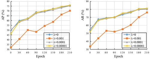
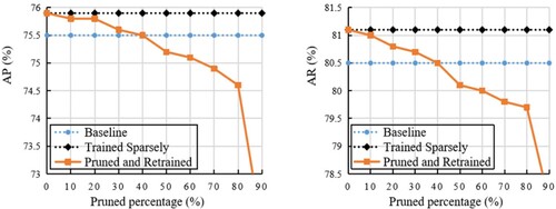
Figure 6. Effect of different pruning rates on model precision.

5.3. Effect of pruned percentage

In pruning work, with an increase in the pruning rate, the parameters and calculation of the model decrease continuously, which achieves the purpose of model compression and acceleration. However, pruning will inevitably affect model performance. The HRNet-W48-384×288 model was pruned with $\lambda =0.00001$ on the COCO dataset to see how different pruning rates affected model precision.

Figure 6 shows that when the pruning rate ranges from 10% to 40%, with an increase in the pruning rate, even if the AP and AR scores of the pruned and retrained model gradually decrease, this model are still higher than the original model on the AP and AR scores. This is most likely due to the regularisation influence of L1 sparsity on weights and channel scaling parameters. Only when the threshold exceeds 40%, the pruned and retrained model are lower than the baseline model on the AP and AR scores. In summary, the original model is pruned with a lower pruning rate, which can restore the model precision to the original model precision after retraining and effectively reduce the model parameters and FLOPs. When the pruning rate is high, pruning the original model will destroy the expressive ability of the model and seriously reduce the model precision. Therefore, we need to select an appropriate pruning rate to prune the original model and accomplish model compression and acceleration maximisation with minimal precision loss.

5.4. Comparison with different pruning approaches

SPM is compared with the latest advanced pruning methods. Tables 3 and 4 provide the comparison results on the COCO and MPII datasets, respectively. The precision drop (AP Drop or AR Drop or [email protected] Drop), the reduction rate of FLOPs, and parameters of the compressed models are all presented in the tables. The best results are shown in bold. For HRNet-W32-384 × 288, we compared with other pruning methods at the operating point of 60% pruned. The approach outperforms the competition in terms of compression rate and precision, according to the comparison. Among them, the compression ratio of parameters and GFLOPs were the highest, 50.5% and 53.7%, respectively. The lowest accuracy rate was 0.9%. On COCO, for the HRNet-W48-384 × 288 task, we set the operating point of 80% pruned for comparison with several methods. The proposed method achieves the maximum compression rate, with a precision drop similar to GBN (You et al., 2019). On MPII, SPM can also achieve better performance than recent advanced approaches. For instance, SPM can reduce the Params by 62.5% and the GFLOPs by 60.0% without an obvious precision drop when pruning HRNet-W32-256 × 256 at a 70% pruning rate. Thus, the viability and superiority of the SPM are confirmed through comparative experiments.

Table 3. Comparing SPM with different pruning methods on the COCO dataset. Best results are bolded.

		Params	GFLOPs	AP Drop	AR Drop
Model	Methods	Reduction (%)	Reduction (%)	(%)	(%)
HRNet-W32-384 × 288	NS (Liu et al., 2017)	45.1	48.3	1.5	1.2
	SFP (He et al., 2018)	40.1	41.1	2.6	2.1
	HRank (Lin et al., 2020)	49.6	40.7	1.7	1.6
	SPM	50.5	53.7	0.9	0.9
HRNet-W48-384 × 288	NS (Liu et al., 2017)	64.2	65.3	1.6	1.5
	HRank (Lin et al., 2020)	62.1	68.1	2.1	1.9
	GBN (You et al., 2019)	60.5	64.2	0.9	0.8
	SPM	71.2	71.7	0.9	0.8

Table 4. Comparing SPM with different pruning methods on the MPII dataset. Best results are bolded.

Model	Methods	Params reduction (%)	GFLOPs reduction (%)	PCKh@0.5drop (%)
HRNet-W32-256 × 256	NS (Liu et al., 2017)	58.3	56.1	1.3
	SFP (He et al., 2018)	50.1	50.7	2.0
	DMCP (Guo et al., 2020)	54.2	55.3	1.2
	SPM	62.5	60.0	0.8

6. Conclusions

SPM is a novel pruning approach for HPE that we present in this paper. The regularisation constraint is applied to the weight of the CL and the scaling parameter of the BNL during the training phase to make the weight sparse. The significance of the corresponding filter is then judged by combining the two-layer sparse information, and the unimportant filter is pruned. On several datasets, we proved that our strategy may greatly lower the computing costs of the latest models without sacrificing precision. Furthermore, our strategy significantly decreases the model’s training cost and size, and the model requires no special libraries/hardware to deploy on mobile devices.

On the one hand, SPM prunes well for specific human pose estimation models, but to be applied to other models, it is necessary to analyze their network structure to further optimise SPM. Therefore, the structure information of different models will be analyzed in the future to further improve the applicability and application scope of SPM. On the other hand, we employ the SPM to compress and accelerate the model. Although the effect is good, there is considerable room for improvement. In the future, we intend to study other effective model compression methods, such as knowledge distillation and quantisation, and combine them to further compress and accelerate the model.

Disclosure statement

No potential conflict of interest was reported by the author(s).

Additional information

Funding

This work has been partially supported by the National Natural Science Foundation of China [grant numbers 61901241, 61871321, 61901436], Open Research Funds of Information Communication Networks and Security Key Laboratory of Shaanxi Province [grant number ICNS201903], and the Key Research Programme of the Chinese Academy of Sciences [grant number XDPB22].

References

- Andriluka, M., Pishchulin, L., Gehler, P. V., & Schiele, B. (2014). 2D human pose estimation: New benchmark and state of the art analysis. 2014 IEEE Conference on Computer Vision and Pattern Recognition (pp. 3686–3693).
- Bianchi-Berthouze, N., & Kleinsmith, A. (2003). A categorical approach to affective gesture recognition. Connection Science, 15(4), 259–269. https://doi.org/10.1080/09540090310001658793
- Bulat, A., & Tzimiropoulos, G. (2017). Binarized convolutional landmark localizers for human pose estimation and face alignment with limited resources. 2017 IEEE International Conference on Computer Vision (ICCV) (pp. 3726–3734).
- Cao, Z., Hidalgo, G., Simon, T., Wei, S.-E., & Sheikh, Y. (2019). Openpose: Realtime multi-person 2D pose estimation using part affinity fields. IEEE Transactions on Pattern Analysis and Machine Intelligence, 43(1), 172–186. https://doi.org/10.1109/TPAMI.2019.2929257
- Changpinyo, S., Sandler, M., & Zhmoginov, A. (2017). The power of sparsity in convolutional neural networks. arXiv preprint arXiv:1702.06257.
- Doshi-Velez, F., & Roy, N. (2008). Spoken language interaction with model uncertainty: An adaptive human robot interaction system. Connection Science, 20(4), 299–318. https://doi.org/10.1080/09540090802413145
- Guo, S., Wang, Y., Li, Q., & Yan, J. (2020). DMCP: Differentiable Markov channel pruning for neural networks. 2020 IEEE/CVF Conference on Computer Vision and Pattern Recognition (CVPR)(pp. 1536–1544).
- Guo, Y., Yao, A., & Chen, Y. (2016). Dynamic network surgery for efficient DNNs. NIPS.
- Han, S., Pool, J., Tran, J., & Dally, W. J. (2015). Learning both weights and connections for efficient neural network. ArXiv, abs/1506.02626.
- He, K., Zhang, X., Ren, S., & Sun, J. (2016). Deep residual learning for image recognition. 2016 IEEE Conference on Computer Vision and Pattern Recognition (CVPR) (pp. 770–778).
- He, Y., Kang, G., Dong, X., Fu, Y., & Yang, Y. (2018). Soft filter pruning for accelerating deep convolutional neural networks. IJCAI.
- He, Y., Zhang, X., & Sun, J. (2017). Channel pruning for accelerating very deep neural networks. 2017 IEEE International Conference on Computer Vision (ICCV) (pp. 1398–1406).
- Ioffe, S., & Szegedy, C. (2015). Batch normalization: Accelerating deep network training by reducing internal covariate shift. ArXiv, abs/1502.03167.
- Jiang, D., Qu, H., Zhao, J.-H., Zhao, J., & Hsieh, M.-Y. (2021). Aggregating multi-scale contextual features from multiple stages for semantic image segmentation. Connection Science, 33(3), 605–622. https://doi.org/10.1080/09540091.2020.1862059
- Kingma, D. P., & Ba, J. (2015). Adam: A method for stochastic optimization. CoRR, abs/1412.6980.
- LeCun, Y., Denker, J. S., & Solla, S. A. (1989). Optimal brain damage. NIPS.
- Li, H., Kadav, A., Durdanovic, I., Samet, H., & Graf, H. P. (2017). Pruning filters for efficient ConvNets. ArXiv, abs/1608.08710.
- Li, S., Ning, X., Yu, L., Zhang, L., Dong, X., Shi, Y., & He, W. (2020). Multi-angle head pose classification when wearing the mask for face recognition under the COVID-19 coronavirus epidemic. 2020 International Conference on High Performance Big Data and Intelligent Systems (HPBD&IS) (pp. 1–5).
- Li, S., Sun, L., Ning, X., Shi, Y., & Dong, X. (2019). Head pose classification based on line Portrait. 2019 International Conference on High Performance Big Data and Intelligent Systems (HPBD&IS)(pp. 186–189).
- Lin, M., Ji, R., Wang, Y., Zhang, Y., Zhang, B., Tian, Y., & Shao, L. (2020). HRank: Filter pruning using high-rank feature map. 2020 IEEE/CVF Conference on Computer Vision and Pattern Recognition (CVPR)(pp. 1526–1535).
- Lin, T.-Y., Maire, M., Belongie, S. J., Hays, J., Perona, P., Ramanan, D., Dollár, P., & Zitnick, C. L. (2014). Microsoft COCO: Common objects in context. ECCV.
- Liu, Z., Li, J., Shen, Z., Huang, G., Yan, S., & Zhang, C. (2017). learning efficient convolutional networks through network slimming. 2017 IEEE International Conference on Computer Vision (ICCV)(pp. 2755–2763).
- Luo, J.-H., & Wu, J. (2017). An entropy-based pruning method for CNN compression. ArXiv, abs/1706.05791.
- Newell, A., Yang, K., & Deng, J. (2016). Stacked hourglass networks for human pose estimation. ECCV.
- Ning, X., Duan, P., Li, W., & Zhang, S. (2020). Real-time 3D face alignment using an encoder-decoder network with an efficient deconvolution layer. IEEE Signal Processing Letters, 27, 1944–1948. https://doi.org/10.1109/LSP.2020.3032277
- Ning, X., Gong, K., Li, W., & Zhang, L. (2021). JWSAA: Joint weak saliency and attention aware for person re-identification. Neurocomputing, 453, 801–811. https://doi.org/10.1016/j.neucom.2020.05.106
- Ning, X., Gong, K., Li, W., Zhang, L., Bai, X., & Tian, S. (2021). Feature refinement and filter network for person re-identification. IEEE Transactions on Circuits and Systems for Video Technology, 31(9), 3391–3402. https://doi.org/10.1109/TCSVT.2020.3043026
- Ning, X., Nan, F., Xu, S., Yu, L., & Zhang, L. (2020). Multi view frontal face image generation: A survey. Concurrency and Computation: Practice and Experience.
- Pishchulin, L., Andriluka, M., Gehler, P. V., & Schiele, B. (2013). Poselet conditioned pictorial structures. 2013 IEEE Conference on Computer Vision and Pattern Recognition (pp. 588–595).
- Scardapane, S., Comminiello, D., Hussain, A., & Uncini, A. (2017). Group sparse regularization for deep neural networks. ArXiv, abs/1607.00485.
- Srivastava, V., & Biswas, B. (2020). CNN-based salient features in HSI image semantic target prediction. Connection Science, 32(2), 113–131. https://doi.org/10.1080/09540091.2019.1650330
- Sun, K., Xiao, B., Liu, D., & Wang, J. (2019). Deep high-resolution representation learning for human pose estimation. 2019 IEEE/CVF Conference on Computer Vision and Pattern Recognition (CVPR)(pp. 5686–5696).
- Sun, X., Wang, Q.-W., Zhang, X., Xu, C., & Zhang, W. (2021). Deep blur detection network with boundary-aware multi-scale features. Connection Science, 1–19. https://doi.org/10.1080/09540091.2021.1933906
- Suzuki, N., & Katagiri, Y. (2007). Prosodic alignment in human computer interaction. Connection Science, 19(2), 131–141. https://doi.org/10.1080/09540090701369125
- Toshev, A., & Szegedy, C. (2014). DeepPose: Human pose estimation via deep neural networks. 2014 IEEE Conference on Computer Vision and Pattern Recognition (pp. 1653–1660).
- Wei, S.-E., Ramakrishna, V., Kanade, T., & Sheikh, Y. (2016). Convolutional pose machines. 2016 IEEE Conference on Computer Vision and Pattern Recognition (CVPR) (pp. 4724–4732).
- Wen, W., Wu, C., Wang, Y., Chen, Y., & Li, H. H. (2016). Learning structured sparsity in deep neural networks. NIPS.
- Wu, Z., Gao, Y., Li, L., Xue, J., & Li, Y. (2019). Semantic segmentation of high-resolution remote sensing images using fully convolutional network with adaptive threshold. Connection Science, 31(2), 169–184. https://doi.org/10.1080/09540091.2018.1510902
- Xu, Z., & Zhang, W. (2020). Hand segmentation pipeline from depth map: An integrated approach of histogram threshold selection and shallow CNN classification. Connection Science, 32(2), 162–173. https://doi.org/10.1080/09540091.2019.1670621
- Yan, C., Pang, G., Bai, X., Zhou, J., & Gu, L. (2020). Beyond triplet loss: Person re-identification with fine-grained difference-aware pairwise loss. ArXiv, abs/2009.10295.
- Yang, Y., & Ramanan, D. (2011). Articulated pose estimation with flexible mixtures-of-parts. CVPR, 2011, 1385–1392.
- Ying, L., Qian Nan, Z., Fu Ping, W., Tuan Kiang, C., Keng Pang, L., Heng Chang, Z., Lu, C., Jun, L. G., & Nam, L. (2021). Adaptive weights learning in CNN feature fusion for crime scene investigation image classification. Connection Science, 33(3), 719–734. https://doi.org/10.1080/09540091.2021.1875987
- You, Z., Yan, K., Ye, J., Ma, M., & Wang, P. (2019). Gate decorator: Global filter pruning method for accelerating deep convolutional neural networks. ArXiv, abs/1909.08174.
- Zhang, L., Li, W., Yu, L., Sun, L., Dong, X., & Ning, X. (2021). Gmface: An explicit function for face image representation. Displays, 68, 102022. https://doi.org/10.1016/j.displa.2021.102022
- Zhang, L., Sun, L., Yu, L., Dong, X., Chen, J., Cai, W., Wang, C., & Ning, X. (2021). ARFace: Attention-aware and regularization for face recognition with reinforcement learning. IEEE Transactions on Biometrics, Behavior, and Identity Science. https://doi.org/10.1109/TBIOM.2021.3104014
- Zhang, Z., Tang, J., & Wu, G. (2019). Simple and lightweight human pose estimation. ArXiv, abs/1911.10346.
- Zhuang, Z., Tan, M., Zhuang, B., Liu, J., Guo, Y., Wu, Q., Huang, J., & Zhu, J.-H. (2018). Discrimination-aware channel pruning for deep neural networks. NeurIPS.