Evaluating performance variations cross cloud data centres using multiview comparative workload traces analysis

Abstract

How to evaluate the performance variations of large-scale cloud data centres is challenging due to diverse nature of cloud platforms. Classic methods such as profiling-based evaluating methods tend to only provide global statistics for a system compared with cloud tracing based approaches. However, existing tracing based research lacks a systematic comparative multiview analysis from architecure-view to job-view and task-view, etc.to evaluate cloud performance variations, together with a detailed case study. We introduce MuCoTrAna, a multiview comparative workload traces analysis approach to evaluate the performance variations of large-scale cloud data centres which assists the cloud platform performance managers and big trace analysts. The efficiency of the proposed approach is demonstrated via case studies in Alibaba 2018 trace and Google trace. The multifaceted analysis results of traces reveals the qualitative insights, performance bottlenecks, inferences and adequate suggestions from global view, machine view, job-task view, etc.

Keywords:

• Evaluating performance variations
• trace analysis
• multiview analysis
• Google trace
• Alibaba trace
• cloud computing

1. Introduction

How to evaluate the performance variations of large-scale cloud data centres (Daid et al., 2021; Guo et al., 2019; Javadpour et al., 2021; Yu et al., 2021; Zhao et al., 2021) is challenging due to diverse nature of cloud platforms. Classic methods such as profiling-based evaluating methods tend to only provide global statistics for a system compared with cloud tracing-based approaches. With increasing diversity and complexity of cloud platforms, diagnosing the performance variations across large-scale cloud platforms by analysing the workload trace of data is gaining attention from research community (Amvrosiadis et al., 2018; Ogbole et al., 2021; Xiao et al., 2021). Amvrosiadis et al. (2018) reported that one challenge in the cluster workload traces analysis is the diversity and hence only using trace from one platform can't show the generality of a technique.Through the analysis of Alibaba trace, Luo et al. (2021) found that most microservices are more sensitive to CPU than memory in Alibaba cluster. Our motivation is based on the urgent need to conduct a detailed analysis by comparing various traces cross platforms. In addition, diagnosing cloud platform performance bottlenecks can be classified into two schemes namely, inner-platform performance analysis and cross-platforms performance analysis. Despite extensive research in the areas of inner-platform performance analysis under single cloud platform (Yu et al., 2021), such as FaceBook trace (Facebook, 2010) and taobao dataset (Ren et al., 2013), the cross-platform quantitative deep performance comparative analysis from multiviews via traces analysis has been overlooked. Moreover, Amvrosiadis et al. (2018) reports that most traces are confidential and therefore cannot be used for comparative studies.

Two of the most representative cloud traces are the Google trace (Google, 2011) which is the classic trace collected in 2011 by Google; and the Ali2018 (Alibaba, 2018) which was released in December 2018. Although multiview learning is effective, it is reported in Amvrosiadis et al. (2018) that there exist hundreds of research articles on Google trace (Peng et al., 2018; Zhang et al., 2016) and Alibaba trace (Guo et al., 2019). However, an empirical study on diagnosing performance variations between Google trace and Ali2018 using a comparative multiview method from overall to detailed tasks is missing. Similarly, although the trace analysis tool is an effective tool for empowering developers to monitor system anomalies and analyse performance bottlenecks without a deeper understanding of the system, the trace analysis tools for the comparative analysis of traces are lacking.

We introduce MuCoTrAna, a multiview comparative workload traces analysis approach for diagnosing performance variations in large-scale cloud data centres. The initial idea of this work was presented in Ruan et al. (2019), which only demonstrates the problem and limited solutions for some initial analysis. In this paper, we systematize our method by extending the background ideas, providing a more comprehensive survey of the recent related work, deepening the design of the architecture and analysis process, and integrating more new interesting findings together with adequate discussion and suggestions. Secondly, we present a comparative empirical study on Google cluster and Ali2018 and reveal several diverse novel interesting findings. Our findings and discussion would be of great interest to cloud traces analysts and platforms managers as such details of practical nature have never been reported before. Performance variations from the global view of data structure, machines, jobs and tasks, etc., are carefully investigated. We also design a multiview comparative workload trace analysis tool that provides a user-friendly unified visual support for comparative, multiview, spatial and temporal analysis of large-scale cloud traces.

The remainder of this paper is organised as follows: Section 2 provides a brief overview of the related work. The design of MuCoTraAna is presented in Section 3. The case study findings and results analysis are carefully studied in Section 4. The design and implementation of the trace analysis tool are presented in Section 5. The paper is concluded in Section 6.

2. Related work

The efficiency of diagnosing performance variations based on trace analysis is determined by traces, relevant methods and applicable tools (Liu & Yu, 2018; Lu et al., 2017; Tang et al., 2021; Xu et al., 2021). In this section, we survey the recent related work on the above aspects.

In the view of the trace data source, Amvrosiadis et al. (2018) reported that most of the traces are still secret and cannot be compared. Google trace was collected in 2011 and Ali2018 was collected in December 2018. They are the most popular representative open-source traces which can be used to demonstrate how to diagnose the variations and evolution between cloud platforms.

In the view of the recent research progress in trace analysis, we classified the recent representative research papers in Google and Alibaba traces in Table 1. First, we analyse the research on Google trace. In the machine view, the existing researches focus more on the heterogeneity of machine configuration and the dynamics of machine resources, e.g. revealed the daily trend of machine events, and Reiss et al. (2012a) found that there were about 40% of the machines unable to be scheduled at least once. In the tasks view, Reiss et al. (2012b), Ruan et al. (2019), Reiss et al. (2012a) and Di et al. (2012) revealed the long tail phenomena in terms of the job scale. For the execution process of jobs and tasks, the existing research reveals that there is a relationship between the trends of the different states of tasks. Liu et al. (2016) proposed that adding machines will reduce the failure rate of the jobs. Gao et al. (2020) analysed the Google trace and proposed a failure prediction algorithm based on a deep learning method to identify task and job failures in the cloud. Reiss et al. (2012a), Reiss et al. (2012b) and Ruan et al. (2019) reported that a few jobs consumed the major amount of the available resources. In the resources view, Reiss et al. (2012a), Reiss et al. (2012b), Chen et al. (2014) and Alnooh and Abdullah (2018) studied the relationship of the CPU and memory of jobs and tasks. Guo et al. (2019), Shan et al. (2018) and Liu and Yu (2018) reported that the modern data centres have the disadvantage of low resource utilisation, which is the main performance bottleneck. Reiss et al. (2012b) investigated the factors that affect the efficiency of system resources. However, there are still some shortcomings in the existing researches. First of all, they did not represent systematic multiview features and the analysis method to diagnosing performance variations based on trace. These studies are also lack of clarity on the resource efficiency of Google trace.

Table 1. Hot spot analysis of the recent research on Google trace and Alibaba trace.

Views	Liu	Reiss	Reiss	Alnooh	Chen	Liu	Minet	Guo	This paper
Heterogeneity based on machine's resource attributes	•	•	•	•		•	•	•	•
Machine's states are dynamic	•	•			•		•		•
The machine events' time series	•								•
The predominant phenomena of short tasks in the job	•	•	•			•	•	•	•
A few jobs contain a lot of tasks	•	•	•			•	•	•	•
A few jobs occupy most of the resources		•	•						•
Failed jobs consume a lot of resources	•				•				•
User info		•	•		•				•
Task classification based on task priority		•	•	•	•		•		•
Task classification based on the ratio of CPU to Memory		•	•	•	•
Duplicate submissions of jobs and tasks		•	•		•			•
The periodicity and daily patterns of workload	•		•					•	•
Low resource utilisation			•			•		•

For Alibaba trace, it is worth noting that a previous version, called Ali2017, of Ali2018 was released by Alibaba company in 2017. Existing research on Alibaba trace focuses on workload analysis and resource utilisation (Guo et al., 2019; Liu & Yu, 2018). Liu and Yu (2018) made a introduction to Ali2017 from batch job, container and server views. Resource utilisation and performance of Alibaba data centres are studied. Based on our survey, we found that like Google, Alibaba also divides jobs into many tasks, has duplicate submissions of jobs and tasks, keep daily patterns of workload, low resource utilisation and so on Guo et al. (2019). A few papers have made a comprehensive deep comparison between Google trace and Alibaba trace. For example, Shan et al. (2018) point out only around half of the CPU and memory are utilised in both Google and Alibaba cluster. Guo et al. (2019), Liu and Yu (2018) and Cheng et al. (2018) also raised this serious performance bottleneck problem. Everman et al. (2021) exposing the problem of insufficient CPU resources for the jobs in Alibaba trace. However, these papers only compare the two traces in terms of workload and resources, they lack a multiview perspective and no tool support. Moreover, their comparison is relatively imbalance with one trace of Google trace or Alibaba trace.

Trace analysis tool is an effective tool to alleviate the challenge of trace data surging, and enabling developers to monitor system anomalies and analyse performance bottlenecks without the detailed information about of the architecture, components, etc. Doray and Dagenais (2017) proposed a tool for highlighting multiple executions of the same task by simplifying the trace analysis process to help the trace analysts to have a deeper understanding of the system. Adhianto et al. (2010) developed a tool for measuring and analysing the performance of compute nodes in HPC clusters. Giraldeau and Dagenais (2015) introduced a new tool that can display the task execution process in the form of a graph model for many tasks in the distributed system. The above tools pay more attention to the tasks in the system, but cannot reflect the other information such as machines and users views. Although Giraldeau and Dagenais (2015) visualised the task execution state, it is limited to the temporal state of the task. In the cloud trace, usually multiple tasks in the job are executed on different nodes, which can reflect the spatial state. Balliu et al. (2016) proposed a tool for big data trace analysis BiDAl (Big Data Analyzer) and apply it only to Google trace but multiple traces. Versluis et al. (2020) surveys the use of workflow trace and introduce the Workflow Trace Archive(WTA), which supports sharing workflow traces in a common, unified format. Fernandez-Cerero et al. (2020) presented a model to automatically retrieve execution workflows of existing data-centre logs by employing process mining techniques which facilitated the analysis of workflows in the data centre.However, other related prototype systems only focus on a certain view of information in the trace, such as workflow, and do not analyse the information in the trace from a multi-dimensional perspective. Compared with these tools, our tools are user-friendly and unified visual support for comparative, multiview,spatial and temporal analysis of large-scale cloud trace.In addition, our tools can help compare the characteristics of different clusters and effectively discover the shortcomings of cloud computing clusters.

To sum up, for diagnosing the performance variations, George Amvrosiadis et al. (2018) suggested that attention should be paid to diversity in trace analysis. However, recent works focus more on inner-platform performance analysis but cross-platforms. Although recently some of them compared two kinds of traces, but their comparison is not deep and balanced enough in multiview comparative study. There lacks a comparative approach which provides a guidance for the system performance analysts. And the trace analysis tool which can support the trace comparative study are even rare. Therefore, we propose to diagnose the cloud platform's variations by comparatively studying the cloud clusters and proposes a tool together with the methods.

3. Design of multiview-based trace data analysis approach- MuCoTrAna

In this section, we introduce MuCoTrAna which diagnoses the cloud performance variations based on a multiview comparative trace data analysis. Section 3.1 introduces the multiview based trace analysis model. The corresponding analysis process is presented in Section 3.2.

3.1. Multiview-based trace analysis model

Classic methods like profiling based diagnosing methods tend to only provide global statistics for a system compared with the Cloud tracing approach. Multiview analysis and learning is effective in other fields. However, existing tracing based research lacks a systematic comparative multiview analysis approach. Therefore, in this section, we introduce a multiview comparative analysis performance variation diagnosing architecture – MucoTrAna.

In cloud trace analysis, the multiview analysis is a cloud trace data analysis from multiple trace feature sets. The cloud cluster trace contains implicit features about tasks, resources, jobs and failures among trace tables. Through the multiview cloud trace analysis, performance variations patterns, e.g. architecture, job scale, resource utility, can be discovered for performance optimisation. To diagnose performance variations between large-scale cloud datacenters, the first challenge is how to organise such multiview data and extract the features from them.

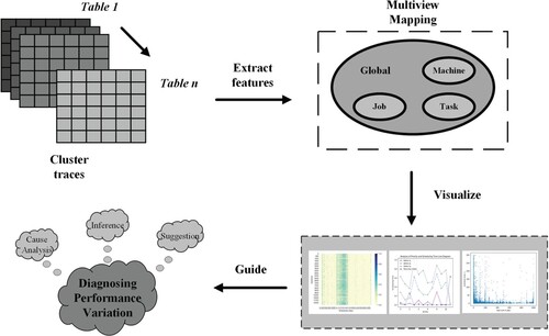
We propose a performance variation diagnosing framework between cloud data centres based on multiview comparative workload analysis (see Figure 1). Based on this framework, we need to establish the mapping by analysing the cluster trace, extract the spacial and temporal distribution features of traces, establish the global views and subviews and then provide the new findings. We diagnose the performance variations by providing the inferences and performance improvement suggestions.

Figure 1. Performance variations diagnosing architecture based on MuCoTrAna.

3.2. Multiview-based trace analysis process

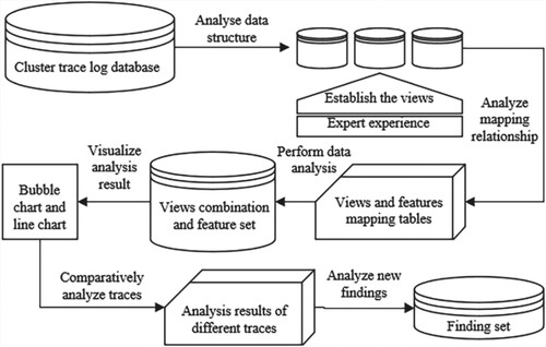
Our multiview-based trace analysis process is presented in Figure 2. To make it clear, we highlight the main steps as follows.

1. Based on the overall view, the trace statistics and data structures are analysed from the trace log database.

2. The spatial and temporal feature views are established based on the trace features and the trace analyst and application expert' knowledge. For example, the machine, job, task and resource usage are usually diagnosed as the most important views in Google trace and Ali2018.

3. The mapping relationship between the views and the trace tables are established by quantitative analysis.

4. The spatial and temporal analysis from multiple views is performed based on the performance optimisation goals.

5. The trace data analysis results are Visualized using the trend analysis, tag cloud analysis, etc.

6. The performance variations between different traces are analysed by the carefully comparisons.

7. The new findings and careful inferences about the performance variations based on the qualitative and quantitative analysis are presented.

Figure 2. The multiview trace analysis based on performance variation diagnosing process.

To better understand the process, a case study together with the results obtained from Google trace and Ali2018 is shown in Section 4. All of the data analyses and new findings are presented based on these two publicly released data sets. Although these two publicly released data sets cannot represent the comprehensive performance trace sets for all cloud platforms, our analysis methods and the finding results can still provide the system analysts a meaningful quantitative scientific deduction method on evaluating the performance of the whole system in the form of a miniature. We believe that the analysis methods and new findings will surely benefit not only the research but also the practitioners' side about the Cloud performance variations diagnosing, performance improving and trace analysis.

4. Case study findings and results analysis

Under the proposed framework and analysis process in Section 3, the data table of Google and Ali2018 according to the global view detailed in Section 4.1 are clarified. From Section 4.2 to 4.4, the Machine analysis, Job analysis and Task analysis will be shown as an example.

4.1. Global view-based data tables classification

The global view-based analysis is performed based on the overall statistics (especially the difference and similarity of scales in the different views) of the traces to be compared for performance variations.

The trace data tables in Google trace and ali2018 according to the views are analysed to establish the mapping relationship based on the framework (Figure 1). As is summarised in Table 2, many interesting findings can be inferred as the following.

Table 2. Feature Comparisons between Google trace and Alibaba trace 2018.

View	Items	Google trace 2011	Alibaba trace 2018
Trace overview	Trace size	41G	49G
	Trace sampling time	29 days	8 days
	Timestamp unit	Microsecond	Second
	Jobs' number	670 thousand	4.2 million
	Tasks' number	25 million	14 million
	Entries' number	1.4 billion	5.6 billion
$\begin{array}{l}\mathrm{Machine}\\ \mathrm{information}\\ \mathrm{analysis}\end{array}$	machines' number	12583	4043
	Machine states	Add, remove, update	Using, import installing
	Machine attribute	CPU, Memory capacity	CPU, Memory, net capacity
Job analysis	Time-sensitive task	Distinguish by scheduling class	Batch tasks, online task
	Task relationship in a job	–	DAG
	entries loss handling	Virtual record	Unprocessed
User	Whether to record user information	Yes	No

• From the sampling day view, Google trace is nearly four times of data per sampling day than Ali2018. We infer that Google trace is somewhat better for those administrators who care about investigating the longer-time system performance analysis based on the trace view than the Ali2018.

• The number of machines on Google's cloud platform is more than three times that of Ali2018. We may infer that the sampling Google platform has bigger machine scale than that of Alibaba cloud.

• The number of tasks per job in Ali2018 is ten times smaller than that in Google trace. We also infer that compared with Google trace, the jobs in ali2018 are divided into smaller granularity tasks on average.

• The information of cluster users can be directly characterised in Ali2018, but Google trace lacks this feature. Such customisation of cluster users may show that the design of Alibaba facilitate its performance based on the users's features.

4.2. The machine-view-based analysis

Machines being the fundamental hardware-level components whose configuration, and events, and so forth, are critical to the cloud platform's performance and thus the focus of our work for diagnosing performance variations.

4.2.1. Machine configuration analysis

In this section, we first investigate the machine configuration. Platform is one important view in large-scale Cloud clusters. We summarise the preliminary statistics on Table Machine events. We can identify that there are four platforms, which are four opaque strings in the Google trace table, named as platform A/B/C/D by us for convenience as shown in Table 3.

Table 3. Resources capacity of platforms in Google trace.

Platform	Machines	CPU	Memory
A	11659	0.5	$\begin{array}{c}0.03\ast 2^n\\ (n<=5),0.5,0.75\end{array}$
B	126	0.25	0.25
C	798	1	1,0.5
D	32	–	–

The main steps of our approach are first traverse the Machine events table; then de-duplicate the Machine events; count out the number of machines by counting the records; finally, the amount of memory resources is obtained from the memory field. Table 3 shows the resources usage from the view of the platform in Google trace.

From Table 3, we find that there are no cases where the machine switches the platform multiple times in the Google platform. In the publicly released traces, the memory capacity data is a normalised value. Thus, all of the memory capacity data have no unit of measurements. In order to study Google's machine resource configuration, we analyse the CPU capacity of all machines in Google trace which has been normalised into three types: 0.25, 0.5 and 1. For the normalised memory capacity, we classify it into four types: [0, 0.25), [0.25, 0.5), [0.5, 0.75), [0.75, 1]. Next, through a statistical analysis of the machine events table, the distribution of the number of machines of the resource capacity is shown in Figure 3 and Table 4.

Figure 3. Machine record number distribution of various resource capacities in Google trace. Bubble size reflects the number of machines.

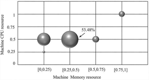
Table 4. Machine resource capacity configuration ($CP{U}_{cap}$, $Me{m}_{cap}$) in Google trace.

$CP{U}_{cap}$	$Me{m}_{cap}$
	$[0,0.25)$	$[0.25,0.5)$	$[0.5,0.75)$	$[0.75,1]$	Total
0.25	126 (1%)	0	0	0	126(1%)
0.5	3924 (31.17%)	6732 (53.48%)	1003 (7.97%)	5 (0.04%)	11664 (92.66%)
1	0	3 (0.02%)	0	795 (6.32%)	798 (6.34%)
Total	4050 (32.17%)	6735 (53.50%)	1003 (7.97%)	800 (6.36%)	12588 (100%)

$CP{U}_{cap}$ denotes CPU Capacity and $Me{m}_{cap}$ denotes Memory Capacity.

In Google trace, most machines (92.66%) are configured with 0.5 CPU capacity, and about half of machines (53.50%) are configured with memory resources in [0.25,0.5) (Table 4). We can infer that in Google trace the CPU and memory capacity of the machine are different. What's more, 53.48% of the machines have the same resource capacity configuration with CPU capacity of 0.5 and memory capacity of [0.25,0.5].

In Ali2018, there are 4043 machines with unique machine_id. By analysing the CPU and memory capacity of Ali2018, we focus on whether Ali2018 has a fine-grained resource management model like Google trace.

From Table 5, we choose the record mem_size and the record cpu_num as the memory capacity index and the CPU capacity index, respectively. We found that the CPU capacity of each machine is 96 cores, and the normalised memory capacity is 100. In Table 5, We can infer that Ali2018 with the same resource capacity configuration may manage CPU capacity and memory resources more coarsely than Google trace with different resource capacity configuration.

Table 5. Homogeneous analysis of Google trace and Ali2018.

Trace	Items
	CPU	Memory	Homogeneous
Google trace	0.25, 0.5, 1	$\begin{array}{c}[0,0.25),\\ [0.25,0.5)\\ [0.5,0.75),\\ [0.75,1]\end{array}$	No
Ali2018	96 cores	100	Yes

4.2.2. Machine events

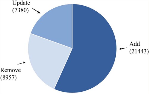
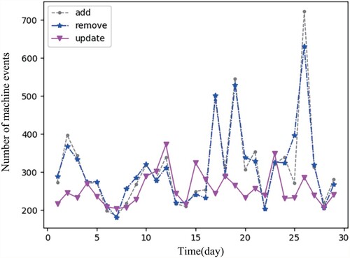
Add, Remove and Update are three types of machine events in Google trace (Figure 4). The Add event occurs when the machine joins a cluster and can perform task. The number of Add records is far more than the other two types of records. Remove event refers to machine failure. There are a total of 8,957 Remove records in Google trace. The Update records are changes to available resources. According the difference of the number of records between Add and Remove, we find that some machines rejoin the cluster after being deleted when running on Google platform.

Figure 4. The event distribution map of each machine in Google trace.

After these statistics, we found that most but not all of the removed machines were need to be added again. 5,141 machines have removal records, and 5,097 machines were removed and again joined to the cluster. The most representative one is the machine with ID 4246147567. It has been performed of 164 times multiple additions and removals. And the machine with ID 6201459631 is 94 times. We record the machine usage time as $T_{use}$, the machine removal time as $T_{remove}$, and the total time as T,M is the machine time usage rate. Here T takes the value of the time of the last record in the $machineevents$ table. (1) $M=T_{use}/T=1-T_{remove}/T$(1) We calculated the M values of the above two machines to be 27.18% and 57.48% by Equation (1(1) $M=T_{use}/T=1-T_{remove}/T$(1) ). From this we can know that frequent removal and addition of machines affects machine utilisation.

Figure 5 shows the trend of three machine events over time in Google trace.Events here represents cumulative events per day. By the analysis of adding and removing records for each machine, we can conclude that 99.14% of the machines are removed and then rejoined into the cluster. On average, each machine is removed and added at a time interval of 4.88 hours, so the line trends of Remove and Add are consistent in Figure 5.

Figure 5. The machine events time series.

There are only two states, Using and Import in Ali2018. The majority state of the machine is Using, and only the machine numbered 2739 has produced 5 records with the state of Import.

Finding 1:

Ali2018 has more coarse-grained resource and event management mechanism than Google trace. Ali2018 is homogeneous, while Google trace is heterogeneous in terms of resource capacity configurations.

Because we know that with the increase of platform scale and application complexity, system software tends to adopt more fine-grained management. We suggest that Alibaba can improve its machine and event management module to support more fine-grained management in its next-generation platform, so as to optimise its performance.

4.3. The jobs and tasks view-based analysis

Job and task scale, scheduling time, resource usage, etc., are key factors to determine the system performance. This section shows our method to analyse the above factors in Google trace and Ali2018.

4.3.1. The job-scale analysis

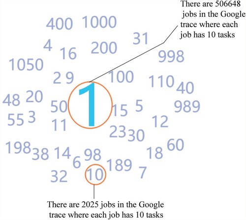
Figure 6 presents the scale of jobs of various sizes in Google trace and Ali2018. It can be seen in Figure 6(a,b), about 75% of the jobs in Google trace contain only one task, while jobs with less than 500 tasks account for more than 98% of the total jobs. From Figure 6(c,d), in Ali2018, 40% jobs in the total of 14 million jobs have only one task, while 99.6% of jobs contain less than 30 tasks. i.e. compared with Google trace, the jobs in Ali2018 tend to be composed of small tasks. We then analyse the task scale by establishing task-scale tag clouds. The job-scale tag cloud for Google trace is depicted in Figure 7. The value of the number represents the job set whose elements are the special job that has the same amount of tasks as the value. E.g. 1 represents the job set whose element is the special job that is composed of single task. 15 represents the job set whose element is a job that is composed of 15 tasks. The size of the number represents the number of job sets whose element contains the same amount of tasks. e.g. The size of 1 in Figure 7 represents there are 506,648 jobs in the Google trace where each job has 1 task. The size of 10 in Figure 7 represents there are 2025 jobs in the Google trace where each job has 10 tasks. From the above comparison, we can find that the size of 1 is much bigger than 10. From Figure 7, we can find that most jobs contain only one task, because the other numbers (like 15,2) are much smaller than 1. It can be also seen that the number of tasks concentrates more on round numbers such as 2, 15, 50, 100, and 1000 in Figure 7. Most of the static task dividing method is based on an integer division dominant mechanism in the Google trace because most of the jobs contain integer (10/100/1000/ 10,000, ect.) tasks.

Figure 6. Google trace and Ali2018 job and task distribution relationship. (a) Frequency distribution of jobs for the specified number of tasks included in Google trace. (b) CDF for jobs with the specified number of tasks in Google trace. (c) Frequency distribution of jobs for the specified number of tasks included in Ali2018 and (d) CDF for jobs with the specified number of tasks in Ali2018.

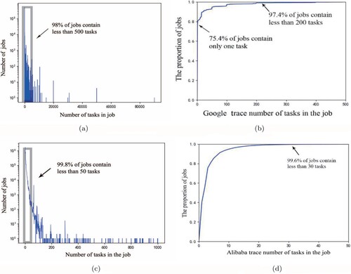
Figure 7. The job-scale tag cloud.

Finding 2:

The majority of the jobs in Google trace and Ali2018 contain only a small amount of tasks. In Google trace, 75% of jobs in Google trace contain only one task, and about 98% of jobs contain less than 500 tasks. In Ali2018, about 99.6% of jobs contained less than 30 tasks. The manual static task dividing method is a major mechanism.

4.3.2. Scheduling time

We record the length of time between task submission and task scheduling as $T_{schedulingtime}$, the timestamp of the task submission is $T_{submit}$, the timestamp of task scheduling is $T_{scheduling}$. (2) $T_{schedulingtime}=T_{scheduling}-T_{submit}$(2) This section mainly explores the distribution of scheduling time in Google trace and the factors that affect scheduling time.

• The relationship of task distribution and scheduling time for scheduling classes

  Table 6 studies the relationship between scheduling class and scheduling time. We provide an algorithm to find the maximum scheduling time by traversal, as shown in Algorithm 1. Its time complexity is $O(n)$. In our research, it needs to run four rounds in total because there are four scheduling classes in Google trace. Initially, we count the total number of tasks for each scheduling class and use the maximum time(MT), average time(AT), less than one second progress($L1$) and more than 1000 s progress($M1000$) as indicators to study the relationship between scheduling time and the task distribution. Taking the column with the scheduling class 0 as an example, $L1$ is 6.91% means that 6.91% of the tasks whose scheduling class is 0 have a scheduling time shorter than 1s. Similarly, for the tasks with scheduling class 0, 28.23% of the tasks scheduling time is shorter than 2s and 62.93% for less than 5s, 2.21% more than 1000s. Figure 8 reflects the relationship between the scheduling time and the distribution of tasks for each scheduling class. From the results in Table 6 and Figure 8, we can draw the following conclusions:

  1. The maximum and average scheduling time for tasks whose scheduling class is three is the smallest.

  2. When the scheduling time is short, compared with tasks whose scheduling class is 0, 1, or 2, the proportion of the tasks whose scheduling classes are three is smaller. However, the scheduling time of the tasks whose scheduling class is three is less than 1000 s.

  It can be concluded that, the higher the scheduling class, the lower the maximum scheduling time and also lower is the probability that the task will starve to death. On the other hand, the average scheduling time is not inversely proportional to the scheduling class.

• The relationship of scheduling time and task priority

  

  Table 7 studies the relationship between priority and scheduling time. We first count the total number of tasks for each priority, and use the six indicators to study the scheduling time distribution. According to the priority value, the priority is divided into five types, which are free ( 0–1), other ( 2–8), normal production (9), monitoring(10), and infrastructure (11). From Table 7 and Figure 9, we have the following findings:

  1. Based on the analysis of the maximum time and average time, we can find that except for the tasks with infrastructure priority, the other tasks with relatively lower priorities like 0, 1, 2 have longer scheduling time than the others.

  2. Although the tasks with priorities from 2-8 belong to the same priority class other, the scheduling time of tasks whose priorities are 3, 5, 6, 7 differs greatly from those tasks whose priorities are 2, 4, 8. The tasks whose priority is 3, 5, 6 or 7, finish their scheduling in such a short time that their scheduling time is all within 1000 s. In contrast, the tasks whose priority is 2, 4, or 8, finish scheduling with longer-time values and hence shortest maximum scheduling time is 16,324 s.

  3. The tasks whose priority is 11 have a maximum scheduling time long up to 20 days while the total sampling time for the whole data set is only 29-days. The average scheduling time of priority 11 is more than 8 h. Moreover, 62.7% of the tasks, whose priority is 11, have a scheduling time which exceeds 1000 s.

  4. It is worth mentioning that the scheduling time follows Pareto's law. As Figure 10 is shown, more than 90% of task scheduling time is shorter than 200s. It means that the scheduling algorithm of Google cluster is relatively effective.

Figure 8. The relationship of task distribution and scheduling time for scheduling classes.

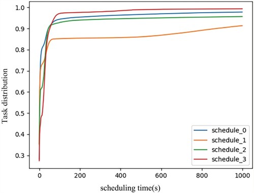
Figure 9. The relationship of scheduling time and priority.

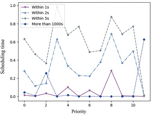
Figure 10. Pareto phenomenon of scheduling time of tasks.

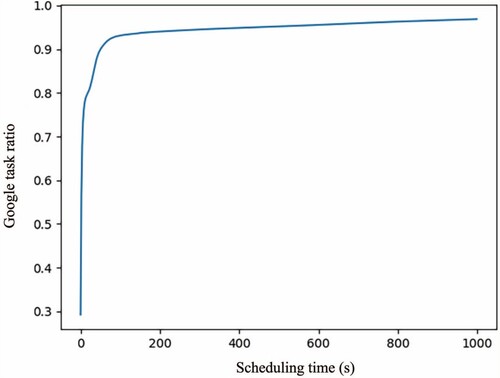
Table 6. Scheduling efficiency in Google trace in terms of scheduling class and scheduling time.

	Scheduling class
Scheduling time	0	1	2	3
Maximum scheduling time	861,225,121,554	480,671,073,268	1,756,309,926,628	23,405,272,151
Average scheduling time	199,923,642	229,361,149	768,879,577	52,226,080
Scheduling time less than 1 s	6.91%	5.97%	4.91%	1.00%
Scheduling time more than 1000 s	2.21%	8.68%	4.34%	0.68%

Table 7. Scheduling efficiency in Google trace in terms of task priority and scheduling time.

	Task priority
Scheduling time	0	1	2	3	4	5	6	7	8	9	10	11
Maximum scheduling time(s)	253975	861225	480671	281	77365	33	343	57	16324	3660	101	1756309
Average scheduling time(s)	269.4	113.71	636.73	2.27	193.13	5.1	9.85	12.32	4.87	11.25	7.33	32066.54
Scheduling time less than one second	1.2%	0.3%	3.3%	0.3%	10.1%	0.0%	6.7%	0.0%	28.3%	0.7%	0.4%	0.0%
Scheduling time more than 1000 s	4.5%	0.8%	25.8%	0.0%	1.5%	0.0%	0.0%	0.0%	0.0%	0.1%	0.0%	62.7%

Considering the above findings, we can deduce that it is opposite to our common intuition that the scheduling time of tasks with higher priority is shorter than those with the lower priority. For example, the task with the priority value of 8, 11 has a higher priority but their scheduling time is not short.

4.3.3. Daily patterns of workloads

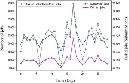
Figure 11 calculated the number of tasks submitted by Google trace and Ali2018 within 24 h. From 1 a.m. to 11 a.m., the number of jobs submitted by Google trace is significantly higher. The number of jobs submitted at 2 a.m. is five times that of jobs submitted at 2 p.m. We conclude that the workload on Google trace is unbalanced at different times on the same day.

Figure 11. Minutely job submission rates for a given day. (a) Finished/submitted/failed tasks time series in Google trace and (b) Submitted tasks time series in Ali2018 trace.

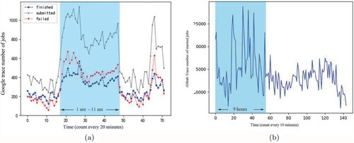
Ali2018 starts at 12am. The number of job submission remained at a high level for 9 h per day. We can deduce that the workload of Ali2018 is uneven. Improving some time-insensitive tasks's spacial locality will improve system performance in both Google trace and Ali2018.

Finding 3:

The workloads of Google trace and Ali2018 vary greatly at different times of the day. The number of tasks submitted by Google trace during peak hours is five times that of idle time. The workload of Ali2018 has maintained a high level of 9 h in 24 h.

From this finding, we think the reason for submitting busy tasks during peak hours can be diagnosed, so that the corresponding measures, such as submission and workload balancing algorithm, can be applied to the platform.

4.4. Task failure analysis

Task failure analysis is an important way to analyse the cause of task failure, improve scheduling and resource allocation, and system efficiency. Although Jassas and Mahmoud (2018) suggests that only 35.91% of the tasks would be successfully completed in the end, it did not report the failure ratio. As can be seen from Figure 12,more than 30% of the jobs failed, including jobs that are evicted, killed, lost or failed. This finding shows that Google trace has a high failure rate of jobs and tasks. Similarly, authors in Garraghan et al. (2014), Chen et al. (2014), Jassas and Mahmoud (2018) and Rosa et al. (2015) performed an analysis of the failure of Google tasks. They mainly analyse the aspects of scheduling class, priority and resource usage. In this paper, in addition to studying the relationship between scheduling classes and priorities for task failure rate in the above sections, we also studied the relationship between machine and task failure.

Figure 12. The failed job ratio in Google trace.

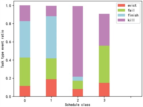
4.4.1. The scheduling class and the events

Figure 13 shows the relationship between various scheduling class and task event type ratio. We observe that for the tasks whose scheduling class is 3, the task completion rate is approximately zero. In addition, the kill rate of the tasks is the largest for the tasks whose scheduling class is 2. The failure rate of the tasks reaches the maximum for the tasks whose scheduling class is 3, which also indicates that the scheduling class will affect the task failure rate. Therefore, we can suggest that in Google's task scheduling, more attention should be paid to tasks whose scheduling class is 3.

Figure 13. The relationship between scheduling class and task events.

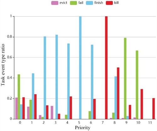
4.4.2. The relationship between event type and task priorities

Figure 14 shows the relationship between various event type ratios and task priorities. The task failure rate first decreases with the increase of priority and then rises. Similar to the scheduling time, the task with the priority classed as other has the lowest task failure rate, and the task with a priority of 5 has a task completion rate of 1. It is worth noting that all submitted tasks with a priority of 7 are killed. We speculate that tasks with too low a priority are more likely to fail when competing for resources resulting in higher failure rates. Tasks with a high priority are highly sensitive to time resulting in higher failure rates.

Figure 14. The relationship between task priority and task events.

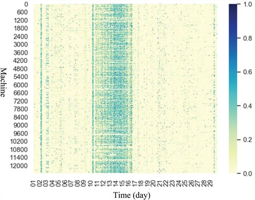
4.4.3. The temporal and spatial characteristics of tasks

In addition to the characteristics of the task itself, the spatial and temporal characteristics also affect the failure rate of the task. Figure 15 shows the task failure rate on 12,583 machines in Google trace within 29 days. We can find that Google trace has a high task failure rate on the 2nd and 10th to 17th days. We deduce that this phenomenon is related to the surge in the number of tasks submitted. This shows that the workload of each machine in the Google cluster has a similar trend. We can propose that if we want to improve the task completion rate, we can submit the batch task in the idle time, and in the event of a surge in workload, we can increase the amount of machines or resources in time so as to reduce the task failure rate.

Figure 15. Heat map of the ratio of failure tasks to submitted tasks.

4.5. The summary of the important findings

For the convenience, we summarise all of the findings from the global views in the following.

• From the sampling day view, Google trace is nearly four times of data per sampling day than Ali2018. We infer that Google trace is somewhat better for those administrators who care about investigating the longer-time system performance analysis based on the trace view than the Ali2018.

• The number of machines on Google's cloud platform is more than three times that of Ali2018. We may infer that the sampling Google platform has a bigger machine scale than that of Alibaba cloud.

• The number of tasks per job in Ali2018 is ten times smaller than that in Google trace. We also infer that compared with Google trace, the jobs in ali2018 are divided into smaller granularity tasks on average.

• The information of cluster users can be directly characterised in Ali2018, but Google trace lacks this feature. Such customisation of cluster users may show that the design of Alibaba facilitates its performance based on the users's features.

We summarise the findings from the subviews in the following:

• Finding 1: Ali2018 has more coarse-grained resource and event manage-ment mechanism than Google trace. Ali2018 is homogeneous, while Googletrace is heterogeneous in terms of resource capacity configurations.

• Finding 2: The majority of the jobs in Google trace and Ali2018 contain only a small amount of tasks. In Google trace, 75% of jobs in Google trace contain only one task, and about 98% of jobs contain less than 500 tasks. In Ali2018, about 99.6% of jobs contained less than 30 tasks. The manual static task dividing method is a major mechanism.

• Finding 3: The workloads of Google trace and Ali2018 vary greatly atdifferent times of the day. The number of tasks submitted by Google traceduring peak hours is five times that of idle time. The workload of Ali2018has maintained a high level of 9 h in 24 h.

5. A multiview comparative analysis based trace analysis tool

We present a design of prototype tool(MuCoTrAna) to provide an unified visual process interface for comparison and analysis of various traces on multiview, spatial, and temporal levels. MuCoTrAna offers trace analysis as well as diagnosing performance variations among large-scale Cloud data centres based on a multiview comparative workload.

In our design idea, cloud performance variation diagnosing tool via trace analysis (e.g. MuCoTrAna) should consist of four layers (Figure 16): Cloud data centres layer, Trace DB layer, Trace Analysis Engine layer, and GUI layer.

Figure 16. The architecture of MuCoTrAna.

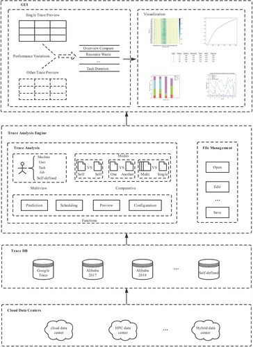
5.1. Cloud data centres layer

Cloud data centres layer is the source of Trace DB layer. It provides detailed chronological workload traces sources.

5.2. Trace DB layer

Trace DB layer contains different traces from various cloud data centres. It stores not only classic traces like Google trace, Alibaba trace 2017, and Alibaba trace 2018, but also some self-defined traces, which aims to enhance the extensibility of the tool in the data source level.

5.3. Trace analysis engine layer

Trace Analysis Engine layer is the core of MuCoTrAna, which includes basic operation and algorithms analysis. The basic operation on traces includes but not limited to open, edit and save traces. The analysis algorithms support multiview and comparative analysis. This engine can execute analysis operations from a single trace to multiple traces. Our tool can operate in three comparative modes: single vs single, single vs another, and single vs multiple. Single vs single compares different attributes in the same trace, i.e. inner-platform performance analysis. Single vs another means to compare the similar attribute between two different traces. While single vs multiple means to compare the attributes in more than three traces. Besides, we incorporate prediction and scheduling functions in the tool.

5.4. The GUI layer

The GUI layer is a user-oriented interface of the tool. Through the graphical interface, the user can easily choose the trace and analyse the trace through mouse clicks. The results of the analysis are displayed in spreadsheets or graphs.

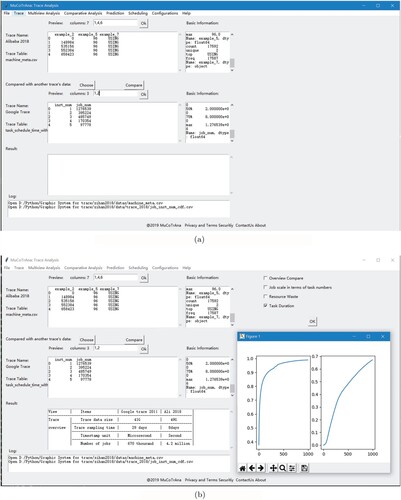
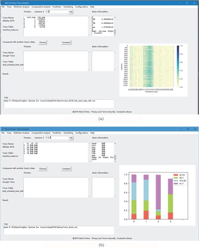
We perform a performance diagnosing case study based on MuCoTrAna in Figures 17and 18. Figure 17 shows the samples of the Ali2018 and Google trace are compared from different aspects. Our tool can also visualise the comparative results for the traces as shown in Figure 18. From the case studies, we show that MuCoTrAna provides support for user-friendly multiview comparative analysis.

Figure 17. The multiview analysis. (a) The overall comparative analysis results of the traces and (b) The long tail analysis of Jobs.

6. Conclusion

We proposed a multiview comparative analysis method and performed a case study on two classical traces: Google trace and Ali2018. Results show that the method can help to point out the good design, bottlenecks, etc., from the architecture-level to machine-level. The comparative empirical study findings can provide insights on how to feature the bottlenecks in cloud big traces. It was found that most of the cloud platforms besides the traces studied in our case study also have the same data items with different item names though and can describe its architecture and resources. We found some interesting findings such as 75% of jobs in Google trace contain only one task, and about 98% of jobs contain less than 500 tasks. In Ali2018, about 99.6% of jobs contained less than 30 tasks. Moreover, our multifaceted analysis and new findings contribute new views about the research in the field of big workload trace data comparative analysis. The current version of our trace prototype tool provides the design where each module is communicated by the computing result value and the output figures. The further improvement of our algorithms, the unified seamless integration of all the modules with the total automatic execution of our big trace analysis process are on our on-going and future work list. The detailed correlation analysis of internal features and external features together with their influence on the performance variations are promising research direction,too.

Figure 18. The sample visual comparative analysis results. (a) The heat map analysis of task failures and (b) the relationship between scheduling class and task events.

Acknowledgments

The authors would like to thank Dong Dai from Department of Computer Science, University of North Carolina at Charlotte, Dolla Mihretu S,and Zihan Ding from Beihang University and Bingdi Tian from Beijing Information Science and Technology University for their valuable comments.

Disclosure statement

No potential conflict of interest was reported by the authors.

Additional information

Funding

This work is supported by the national key research and development program of China (No. 2019YFB1705903), and the NSFC (national science foundation of China) project (No. 62173023 and 92167108), the fund of the State Key Laboratory of Software Development Environment (No.  SKLSDE-2022ZX-6), and the yunnan key laboratory of  blockchain application technology (Project no. YNB202114 of 202105AG070005).

References

- Adhianto, L., Banerjee, S., Fagan, M., Krentel, M., Marin, G., Mellor-Crummey, J., & Tallent, N. R. (2010). HPCToolkit: Tools for performance analysis of optimized parallel programs. Concurrency and Computation: Practice and Experience, 22(6), 685–701. https://doi.org/10.1002/cpe.1553
- Alibaba (2018). Alibaba cluster-data. Retrieved November 5, 2021, from https://github.com/alibaba/clusterdata/.
- Alnooh, A. H. A., & Abdullah, D. B. (2018). Investigation and analysis of Google cluster usage traces: Facts and real-time issues. In 2018 International Conference on Engineering Technology and Their Applications (IICETA) (pp. 60–65). IEEE.
- Amvrosiadis, G., Park, J. W., Ganger, G. R., Gibson, G. A., Baseman, E., & DeBardeleben, N. (2018). On the diversity of cluster workloads and its impact on research results. In 2018 {USENIX} Annual Technical Conference ({USENIX};{ATC} 18) (pp. 533–546). USENIX Association.
- Balliu, A., Olivetti, D., Babaoglu, O., Marzolla, M., & Sîrbu, A. (2016). A big data analyzer for large trace logs. Computing, 98(12), 1225–1249. https://doi.org/10.1007/s00607-015-0480-7
- Chen, X., Lu, C. D., & Pattabiraman, K. (2014). Failure analysis of jobs in compute clouds: A Google cluster case study. In 2014 IEEE 25th International Symposium on Software Reliability Engineering (pp. 167–177). IEEE.
- Cheng, Y., Chai, Z., & Anwar, A. (2018). Characterizing co-located datacenter workloads: An Alibaba case study. In Proceedings of the 9th Asia-Pacific Workshop on Systems (p. 12). ACM.
- Daid, R., Kumar, Y., Hu, Y. C., & Chen, W. L. (2021). An effective scheduling in data centres for efficient CPU usage and service level agreement fulfilment using machine learning. Connection Science, 33(4), 954–974. https://doi.org/10.1080/09540091.2021.1926929
- Di, S., Kondo, D., & Cirne, W. (2012). Host load prediction in a Google compute cloud with a Bayesian model. In Proceedings of the International Conference on High Performance Computing, Networking, Storage and Analysis (p. 21). IEEE/ACM.
- Doray, F., & Dagenais, M. (2017). Diagnosing performance variations by comparing multi-level execution traces. IEEE Transactions on Parallel and Distributed Systems, 28(2), 462–474. https://doi.org/10.1109/TPDS.2016.2567390
- Everman, B., Rajendran, N., Li, X., & Zong, Z. (2021). Improving the cost efficiency of large-scale cloud systems running hybrid workloads-A case study of Alibaba cluster traces. Sustainable Computing: Informatics and Systems, 30. https://doi.org/10.1016/j.suscom.2021.100528.100528.
- Facebook (2010). Facebook workloads repository. Retrieved November 5, 2021, from https://github.com/SWIMProjectUCB/SWIM/wiki/Workloads-repository
- Fernandez-Cerero, D., Gómez-López, M. T., & Alvárez-Bermejo, J. A. (2020). Measuring data-centre workflows complexity through process mining: The Google cluster case. The Journal of Supercomputing, 76(4), 2449–2478. https://doi.org/10.1007/s11227-019-02996-2
- Gao, J., Wang, H., & Shen, H. (2020). Task failure prediction in cloud data centers using deep learning. 2019 IEEE International Conference on Big Data, Los Angeles, CA, USA, December 9–12, 2019.
- Garraghan, P., Moreno, I. S., Townend, P., & Xu, J. (2014). An analysis of failure-related energy waste in a large-scale cloud environment. IEEE Transactions on Emerging Topics in Computing, 2(2), 166–180. https://doi.org/10.1109/TETC.2014.2304500
- Giraldeau, F., & Dagenais, M. (2015). Wait analysis of distributed systems using kernel tracing. IEEE Transactions on Parallel and Distributed Systems, 27(8), 2450–2461. https://doi.org/10.1109/TPDS.2015.2488629
- Google (2011). Google cluster-data. Accessed November 5, 2021, from https://github.com/google/cluster-data.
- Guo, J., Chang, Z., Wang, S., Ding, H., Feng, Y., Mao, L., & Bao, Y. (2019). Who limits the resource efficiency of my datacenter: An analysis of Alibaba datacenter traces. In Proceedings of the International Symposium on Quality of Service (p. 39). ACM.
- Jassas, M., & Mahmoud, Q. H. (2018). Failure analysis and characterization of scheduling jobs in Google cluster trace. In Iecon 2018-44th Annual Conference of the IEEE Industrial Electronics Society (pp. 3102–3107). IEEE.
- Javadpour, A., Saedifar, K., Wang, G., Li, K. C., & Saghafi, F. (2021). Improving the efficiency of customer's credit rating with machine learning in big data cloud computing. Wireless Personal Communications, 121(4), 2699–2718. https://doi.org/10.1007/s11277-021-08844-y
- Liu, B., Lin, Y., & Chen, Y. (2016). Quantitative workload analysis and prediction using Google cluster traces. In 2016 IEEE Conference on Computer Communications Workshops (Infocom Wkshps) (pp. 935–940). IEEE.
- Liu, Q., & Yu, Z. (2018). The elasticity and plasticity in semi-containerized co-locating cloud workload: A view from Alibaba trace. In Proceedings of the ACM Symposium on Cloud Computing (pp. 347–360). ACM.
- Lu, C., Ye, K., Xu, G., Xu, C. Z., & Bai, T. (2017). Imbalance in the cloud: An analysis on alibaba cluster trace. In 2017 IEEE International Conference on Big Data (Big Data) (pp. 2884–2892). IEEE.
- Luo, S., Xu, H., Lu, C., Ye, K., Xu, G., Zhang, L., Ding, Y, He, J, & Xu, C. (2021). Characterizing microservice dependency and performance: Alibaba trace analysis. In Proceedings of the ACM Symposium on Cloud Computing (pp. 412–426). ACM.
- Ogbole, M., Ogbole, E., & Olagesin, A. (2021). Cloud systems and applications: A review. International Journal of Scientific Research in Computer Science, Engineering and Information Technology, 142–149. https://doi.org/10.32628/IJSRCSEIT
- Peng, C., Li, Y., Yu, Y., Zhou, Y., & Du, S. (2018). Multi-step-ahead host load prediction with GRU based encoder-decoder in cloud computing. In 2018 10th International Conference on Knowledge and Smart Technology (KST) (pp. 186–191). IEEE.
- Reiss, C., Tumanov, A., Ganger, G. R., Katz, R. H., & Kozuch, M. A. (2012a). Heterogeneity and dynamicity of clouds at scale: Google trace analysis. In Proceedings of the Third ACM Symposium on Cloud Computing (p. 7). ACM.
- Reiss, C., Tumanov, A., Ganger, G. R., Katz, R. H., & Kozuch, M. A. (2012b). Towards understanding heterogeneous clouds at scale: Google trace analysis. Intel Science and Technology Center for Cloud Computing, Tech. Rep, 84, 1–12.
- Ren, Z., Wan, J., Shi, W., Xu, X., & Zhou, M. (2013). Workload analysis, implications, and optimization on a production hadoop cluster: A case study on taobao. IEEE Transactions on Services Computing, 7(2), 307–321. https://doi.org/10.1109/TSC.4629386
- Rosa, A., Chen, L. Y., & Binder, W. (2015). Understanding the dark side of big data clusters: An analysis beyond failures. In 2015 45th Annual IEEE/IFIP International Conference on Dependable Systems and Networks (pp. 207–218). IEEE.
- Ruan, L., Xu, X., Xiao, L., Yuan, F., Li, Y., & Dai, D. (2019). A comparative study of large-scale cluster workload traces via multiview analysis. In 2019 IEEE 21st International Conference on High Performance Computing and Communications; IEEE 17th International Conference on Smart City; IEEE 5th International Conference on Data Science and Systems (HPCC/SMARTCITY/DSS) (pp. 397–404). IEEE.
- Shan, Y., Huang, Y., Chen, Y., & Zhang, Y. (2018). Legoos: A disseminated, distributed {OS} for hardware resource disaggregation. In 13th {USENIX} Symposium on Operating Systems Design and Implementation ({OSDI} 18) (pp. 69–87). USENIX Association.
- Tang, B., Tang, M., Xia, Y., & Hsieh, M. Y. (2021). Composition pattern-aware web service recommendation based on depth factorisation machine. Connection Science, 33(4), 870–890. https://doi.org/10.1080/09540091.2021.1911933
- Versluis, L., Mathá, R., Talluri, S., Hegeman, T., Prodan, R., Deelman, E., & Iosup, A. (2020). The workflow trace archive: Open-access data from public and private computing infrastructures. IEEE Transactions on Parallel and Distributed Systems, 31(9), 2170–2184. https://doi.org/10.1109/TPDS.71
- Xiao, T., Han, D., He, J., Li, K. C., & de Mello, R. F. (2021). Multi-Keyword ranked search based on mapping set matching in cloud ciphertext storage system. Connection Science, 33(1), 95–112. https://doi.org/10.1080/09540091.2020.1753175
- Xu, J., Xiao, L., Li, Y., Huang, M., Zhuang, Z., Weng, T. H., & Liang, W. (2021). NFMF: neural fusion matrix factorisation for QoS prediction in service selection. Connection Science, 33(3), 753–768. https://doi.org/10.1080/09540091.2021.1889975
- Yu, L., Duan, Y., & Li, K. C. (2021). A real-world service mashup platform based on data integration, information synthesis, and knowledge fusion. Connection Science, 33(3), 463–481. https://doi.org/10.1080/09540091.2020.1841110
- Zhang, W., Li, B., Zhao, D., Gong, F., & Lu, Q. (2016). Workload prediction for cloud cluster using a recurrent neural network. In 2016 International Conference on Identification, Information and Knowledge in the Internet of Things (IIKI) (pp. 104–109). IEEE.
- Zhao, H., Yao, L., Zeng, Z., Li, D., Xie, J., Zhu, W., & Tang, J. (2021). An edge streaming data processing framework for autonomous driving. Connection Science, 33(2), 173–200. https://doi.org/10.1080/09540091.2020.1782840