Predicting before acting: improving policy quality by taking a vision of consequence

Abstract

Deep reinforcement learning has achieved great success in many fields. However, the agent may get trapped during the exploration, lingering around feckless states that pull the agent away from optimal policies. Thus it's worth studying how to improve learning strategies by forecasting future states. To solve the problem, an algorithm that predicts behaviour consequences before taking action, referred to as Thinking about Action Consequence (TAC), based on the combination of the current state and the policy, is proposed. Deep reinforcement learning approaches equipped with TAC take advantage of the intrinsic prediction framework of TAC as well as bad consequence experiences to determine whether to continue exploring the current region or to evade the potential undesired state discriminated by TAC and instead turn to explore other areas. Since TAC will modify the future plan according to the execution of the policy and the changes of the environment, considering the consequences enables the agent to carry out a suitable exploration mechanism, leading to better performance. Compared with traditional Deep Q Learning (DQN), Double DQN, Dueling DQN, Prioritised Experience Replay DQN, and Intrinsic Reward (IR) methods with uncertain stimulus exploration, our TAC method shows better performance in Atari and Box2d environments.

Keywords:

• Reinforcement learning
• policy optimisation
• exploration
• belief representation
• prediction

1. Introduction

Reinforcement Learning (RL) is a learning process that seeks the maximum cumulative reward by interacting with the environment (Feng & Xu, 2017; Lee et al., 2012), where the agent learns from the mapping of actions to states, indicating that the agent is not directly instructed which action to choose, but finds out which action can get the maximum return through continuous trial and error (Mnih et al., 2016). Since RL is sensitive to rewards from the environments, it gradually forms the rewards' expectation and seeks the optimal strategy. Since RL is characteristic pursuing the best stimulation, it has opened many new applications in health care, robotics, intelligent grid, finance, and so on Arulkumaran et al. (2017) and Xu et al. (2014). Deep Reinforcement Learning (DRL) is a new subject that combines deep learning and RL, incorporating the perceptual ability of deep learning (R. W. Wang et al., 2016; Z. Zhang et al., 2020) with the decision-making ability of RL (Lillicrap et al., 2016). As a method close to the human thinking mechanism (Arulkumaran et al., 2017; Li & Li, 2018), it uses the powerful function approximation ability of deep learning to replace the manually specified features, which solves the problem that large-scale data is difficult to be processed. However, DRL still has some issues to solve, e.g. unbridled exploration of the environment, without thinking carefully about the consequence, not wastes a lot of time, degrades the final performance, and gives rise to uncertainty and risk of the model.

There is an old saying: think twice before acting. We all believe that considering the consequence of our behaviour as much as possible, rather than arbitrarily acting, contributes to making a better decision. In standard RL algorithms, to reach the vision (the final goal of the agent wants), it is necessary to know much about the environment so that we have to explore it continually. The exploration phase of a strategy usually tends to be stochastic and coarse, especially in complex and random environments. The more time agents spend exploring, the greater the probability of encountering spaces that cause danger and areas disturbed by noise. As the agent develops a global understanding of the environment, we expect the agent to combine advanced planning with dynamic changes in the environment and create new plans with full consideration of the present and future situation. If the agent can “know” the future state of the action in advance (Haber et al., 2018) and uses it to instruct the selection of the current action, the decision-making ability of the agent can be greatly improved (Burda et al., 2018). In some practical application scenarios, there will be some explorations that bring bad consequences (Mnih et al., 2013) which need to be avoided in the control process (Henaff, 2019). If they are not taken into account, it is likely to lead to task failure. Therefore, the advanced agent is supposed to have the ability to predict the possible bad consequences in the environment in advance (Nair et al., 2018; Ostrovski et al., 2017; Pathak et al., 2019). The agent can consider the future feedback results and then avoid the wrong behaviour and choose the right one. For example, when someone plays Go, a complex checkerboard game, they naturally sketch the future state of the board and then make a beneficial choice. An experienced player will think about the opponent's action, predict the possible landing options for both sides, and use the prediction to determine current landing options. If we have a plan for the future, it is natural for us to choose the more favourable actions (Gidaris et al., 2018; Gregor et al., 2015). We expect that the agent also can construct predictions of future situations that are used to guide the current behaviour of the agent. When the agent interacts with the environment and faces the action selection, it will take the initiative to outline the future picture. According to the future vision, if the vision indicates bad consequences, the agent will give up the initial action and choose other actions. However, few RL algorithms are concerned with predicting the future. (Fujimoto et al., 2018; Haarnoja et al., 2018; Silver et al., 2014).

To solve the problem, we propose a method that promotes exploration by predicting the future consequences of the action, referred to as Thinking about Action Consequence(TAC). The agent of most RL algorithms takes the cumulative reward as a long-term goal and generates a reward and an instant effect after each action execution (Pathak et al., 2018). Our approach is to improve the cumulative reward of the agent by incorporating a predictive framework, taking into account the changes in the environment and the current strategy, and by increasing the instant effect of each step. When the agent carries out exploring, the TAC method is used to promote benign exploration. As it is known that reward shaping can enhance the exploration of agents, there are many studies on how to take advantage of it. For example, Ermolov and Sebe (2020) constructed the intrinsic reward based on uncertainty to boost interactions with the environment. Therefore, we incorporated the Intrinsic Reward (IR) with compared baseline algorithms.

Our contributions in this study include, add a way to evaluate behaviour by predicting the corresponding consequence, and, at the same time, keeps the ability to explore the unknown world to find out novelty and obtain a more comprehensive observation of the environment, which is the process of understanding the world where the desired rewards and unwanted traps coexist. TAC not only harmonises exploration and exploitation but also improves exploration quantity. TAC method into conventional deep RL algorithms to be sensitive to inappropriate policy to push the agent away from bad consequence space, improving overall performance.

The paper is organised as follows: related work is introduced in Section 2; the principle and implementation of TAC are depicted in Section 3; experimental settings are elaborated in Section 4; the experimental results, as well as analysis, are discussed in detail in Section 5; the benefits of the TAC are outlined, and an outlook for the future is presented in Section 6.

2. Related work

2.1. Deep reinforcement learning

Q-learning Q-learning (Abed-alguni & Ottom, 2018; Watkins & Dayan, 1992) is a value-based RL algorithm that searches for a policy that instructs the agent to act at each time step and evaluates the policy with the state-action function. Q-learning uses experience and selects the action with the highest performance expectation with updating function as: (1) $Q(S_t,A_t)\leftarrow Q(S_t,A_t)+\alpha [R_{t+1}+\gamma \underset{a}{max}Q(S_t,a)-Q(S_t,A_t)]$(1) where $R_{t+1}$ is the subsequent reward, α is the learning rate, γ is the discount factor, and $Q(S_t,A_t)$ is the future value expectation of action $A_t$ taken by $S_t$ in the current state. From Equation (1(1) $Q(S_t,A_t)\leftarrow Q(S_t,A_t)+\alpha [R_{t+1}+\gamma \underset{a}{max}Q(S_t,a)-Q(S_t,A_t)]$(1) ), it can be observed that a larger discount factor γ improves the influence of $\underset{a}{max}Q(S_t,a)$, which also indicates that it would be more influenced by experience. Q-learning belongs to the off-policy method because the update value function does not completely follow the interaction sequence but selects the interaction sequence sub-part from other policies to replace the original interaction sequence. The idea of Q-learning combines the optimal value of the sub-part, hoping to use the optimal value of the previous iteration part to update each time.

DQN and its varieties Deep Q Network (DQN) (Mnih et al., 2013) is a classic combination of RL and deep learning, which has performed well in the Atari environment, even reaching expert levels in some tasks (Mnih et al., 2013). The main innovation of DQN is experience replay and setting up a separate target network that breaks the correlation by using experience playback, which reduces the fluctuation of the value function model, and then set a different target network to reduce the instability of the Q-value updating. The state-value function is as follows: (2) $Y_t^{DQN}=R_{t+1}+\gamma \underset{a}{max}Q(S_{t+1},a;{\theta }_t^{-})$(2) where the Q function is approximated by a neural network, the input is the following state, and the return is the largest state value function corresponding to all actions.

Double DQN Double DQN (DDQN) (Hasselt et al., 2016) has two Q-network models, a target Q-network and a current Q-network, where the target Q-network is used to select actions, and the current Q-network is used to choose Q-value. DDQN does not search for the maximum value through the target Q-network but finds the action corresponding to the maximum Q-value in the current Q-network. Then, it put the selected effort into the target network to calculate the Q-value, solving the overestimation problem in DQN. The state-value function is as follows: (3) $Y_t^{DDQN}=R_{t+1}+\gamma Q(S_{t+1},\underset{a}{\mathrm{argmax}}Q(S_{t+1},a;\theta );{\theta }^{-})$(3) where the current $Q(;\theta )$ network selects the action of maximum Q value, and the target Q value is calculated in the target network $Q(;{\theta }^{-})$.

Dueling DQN In order to distinguish the effects of different actions under the same state, Dueling DQN (DuDQN) is proposed to decompose $Q(s,a)$ into two parts and uses state value and action advantage to synthesise Q value to enhance the influence of action on the agent (Z. Wang et al., 2016). The state-value function is as follows: (4) $Q(S,A,\omega ,\alpha ,\beta )=V(S,\omega ,\alpha )+A(S,A,\omega ,\beta )$(4) where V is the value function, A is the advantage function, ω is a standard parameter, α is the parameter independent of the value function, and β is the parameter independent of the advantage function.

Prioritised Experience Replay DQN In the traditional DQN algorithm, the data of the experience pool are usually randomly sampled. However, it is not always the case as influences to the model caused by the priority of experiences varied.

Prioritised Experience Replay DQN(PerDQN) (Schaul et al., 2016) uses TD error to divide the sample data in the experience pool. The experience with more significant TD error is assigned with higher priority and vice versa. The concept of the primary experience method proposed by PerDQN enabled agents to learn from more valuable data in the samples, which further improved the performance.

2.2. Partially observable Markov decision process

The standard Markov Decision Processes(MDP) is infeasible in the partially observable environment: agents could not confirm their location and state because the environment was not fully visible. To solve partially observable environments, Partially Observable Markov Decision Process (POMDP) (Liang et al., 2019), the generalisation of MDP, is proposed which simulated agent decision-making process was by assuming that the system conformed to MDP (Z. Z. Zhang et al., 2014, 2015). However, agents could not directly observe the state and must continually update their understanding of the global environment from the partial observation information collected in POMDP (Lim et al., 2020). Because the agent could not observe the overall environment, it could not confirm its state. Instead, agents needed to collect environmental information to determine their state constantly.

POMDP is modelled by a seven-tuple ($S,A,P,R,\mathrm{\Omega },O,\gamma$) where S denotes the state space; A denotes the state or action space; P denotes the state transfer function; R denotes the reward function; Ω denotes a set of observations obtained by the agent; O is the conditional observation probability, showing how likely the agent determines that it is in state s after observing the environmental data; γ is the discount factor and $0\le \gamma \le 1$.

One of the advantages of the POMDP perspective is that the uncertainty of the state is clarified in the partially observable environment. Belief state is based on the historical sequence ($h_t={\mathrm{\Omega }}_0,a_0,{\mathrm{\Omega }}_1,a_1,\dots ,a_{t-1},{\mathrm{\Omega }}_t$) to confirm the probability of the current state, i.e. $P_b(|h_t)$). In partially observable environments, POMDP and belief state are proposed to eliminate uncertainty and thus determine where the intelligence is located, which allowed RL algorithms applicable on MDP to be used on POMDP, extending the adaptability of RL to the environment. The Bayesian method could be used to solve the trade-off between exploration and exploitation in RL, but it needs to be in a completely observable environment. To use the Bayesian model in a partially observable environment, Katt et al. (2019) propose the factored Bayes adaptive POMDP model by using POMDP modelling, which could be learned in a partially observable environment. Belief states could capture the distribution of latent states in POMDP. Gangwani et al. (2019) study the belief state problem of Generative Adversarial Imitation Learning (GAIL) in POMDP and combines belief module and strategy to ensure the strategic goal by using task-based imitative loss, which has better performance than the original GAIL algorithm.

2.3. Reward shaping

RL has been proved to be effective in recent years in dealing with complex environments. However, it requires heavy computation because, to understand the environment, agents must perform a large amount of exploration, resulting in low sample utilisation, especially in sparse environments where the time spent by the agent interacting with the environment is catastrophic.

A common approach to accelerate interaction is to use reward shaping (Marom & Rosman, 2018), where the ultimate goal is approached step by step through a well-designed reward function which, however, has difficulty for complex environments. Goyal et al. (2019) propose the Language-Action Reward Network (LEARN), which maps natural language instructions to intermediate rewards that agents should take and is easily scalable to any standardised RL algorithms, and achieves good performance in Montezuma's revenge environment. Marom and Rosman (2018) put forward a Bayesian reward shaping framework, which utilises the decay of experience to design reward distributions in the Q-leaning algorithm. Ermolov and Sebe (2020) use a self-supervised representation learning method for image-based observations, which primarily exploits uncertainty to guide exploration and uses Whitening Mean Square Error(MSE) loss to handle uncertainty and construct intrinsic rewards. Reward shaping improves the efficiency of interaction, sample utilisation, and final performance.

2.4. Exploration and prediction

A successful RL approach requires a global understanding of the environment, so the agent is supported to explore the environment adequately by trial and error mechanism. However, it was more challenging to capture the global view of the environment in partially observable environments due to its unpredictability, which requires learning a representation about the future to explore.

To better obtain the information of the world and determine the state of an agent, belief state is utilised to understand the basic information of the world, which makes use of the historical information of the past $h_t=(s_0,a_0,s_1,a_1,\dots ,s_{t-1},a_t)$ and the future action sequence $A_{t:t+k}=(a_t,a_{t+1},\dots ,a_{t+k-1})$ to predict the future. Moreno et al. (2018), He et al. (2016), and Higgins et al. (2017) use belief state and future action sequence $A_{t:t+k}$ to predict the location and direction of the agent; Azar et al. (2019), Frank et al. (2014) propose Neural Different Information Gain Optimisation (NIDGO) solve the problem that when there are few reward signals from external environments, agents are easily affected by white noise and lose their overall understanding of the world. Using prediction error as information gain, the agent could be free from the influence of white noise; Hafner et al. (2018) introduce a deep Planning Network (PLANET) using prediction, which learns environment dynamics from images, and by combining with Model-Predictive Control(MPC) method where the action was selected by rapid planning in the potential space; Haber et al. (2018) uses curiosity to construct a world model to predict the action consequences of agents in the environment without external rewards and proposes a self-model to select actions; Sekar et al. (2020) put forward latent disagreement with the concept, and additional environment model is used to solve retrospective novelty, utilising the model put forward by the Plan2Explore to solve the specific rewards problem, improving the model's generalisation.

In conventional exploration tasks, the agent often falls into the useless trap and is affected by white noise, which results in the agent wasting a lot of time to carry out fruitless exploration, which wastes time and leads to severe performance degradation. Fortunately, the use of historical information for the forward prediction helps to escape from the dilemma. It is possible to determine the future difficulty through prediction and then use the information to avoid bad consequences or useless explorations.

3. Method

3.1. System architecture

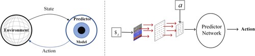
Unlike conventional RL methods, the agent weighs exploitation and exploration during interaction with the environment and makes foresight moves in response to random exploration. To allow agents to predict the future and make plans adequately, we propose TAC. The system architecture is shown in Figure 1. The primary purpose of this method is to establish a forward prediction model based on bad states by collecting bad consequence samples, identifying the future bad states and avoiding them, and guiding the agent to explore more efficiently.

Figure 1. TAC interacts with the environment. The agent obtains the state $s_t$ in the environment, combines the initial exploration strategy action to predict the future state, and selects the final action by predictor model in combination with environmental changes.

3.2. Prediction framework

The trade-off between exploration and exploitation has always been a challenge. A thorough understanding of the environment requires continuous exploration. Otherwise, agents may fall into local optimums, while unlimited exploration may attract the agent by traps or white noise.

In the deep Q network, the most common exploration strategy is the $ϵ-greedy$ strategy, which is usually implemented in the first exploration stage. The agent gives more exploration value so that the agent can collect sufficient information about the environment. In the second stage of exploration, because the agent has already had much understanding of the environment, it gradually less explores and increases the utilisation to make the agent more inclined to capture the reward. However, it is hard to determine the terminal of the first stage. The agent still spends a lot of time exploring even when the focus has already transferred to exploitation, resulting in slow and inefficient convergence.

Our method adds predictive control to exploration, where the prediction framework is mainly composed of a Gated Recurrent Unit (GRU) network and a full connection layer. A forward prediction model is sensitive to the critical state through the pool of bad consequences, including the trap in the task and the crucial state before the failure of the task. To describe our approach more clearly, we have concisely presented the system model variables see Table 1.

Table 1. Introduction of system model variables.

Variables	Description
ω	Discriminator: judgment of prediction results
ψ	Controller: Select final action based on predicted consequences
GRU	Gated Recurrent Unit
MLP	Two fully-connected layers are composed for prediction
$b_t$	Hidden state
${\overline{s}}_{t+1}$	Predicted future state
z	Prediction of consequences, 0 means good, 1 means bad
$D_1$	Experience replay buffer
$D_2$	The experience replay buffer of bad consequence
$L_2$	Loss of mean squared error
ℓ	Prediction network objective function

The training We collect $(s_t,a,s_{t+1})$ from the experience replay buffer of bad consequence $D_2$ and acquire hidden states $b_t$ through GRU network: (5) $b_t=GRU(s_t,a_t)$(5) where $b_t$ contains historical information and the future state ${\overline{s}}_{t+1}$ is predicted through MLP (see Section 4 for detailed information): (6) ${\overline{s}}_{t+1}=MLP(b_t,a_t)$(6) The objective function ℓ is the squared error between the predicted future state ${\overline{s}}_{t+1}$ and actual future state $s_{t+1}$: (7) $\ell =L_2({\overline{s}}_{t+1},s_{t+1})$(7) where $L_2$ is a squared loss function, so that the prediction network can predict future states more accurately.

Using the data from $D_2$ to train, combined with the GRU network to obtain the hidden states, we can get a future-sensitive predictive network model by which we can know the future conditions.

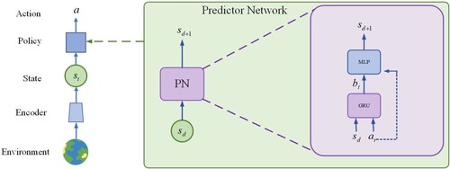
The samples for the prediction model are collected along with the interaction with the environment. Since the deep Q network embodies the trade-off of exploration and exploitation, during the stochastic exploration, the predicted danger state is compared with the bad consequence sample, and the discriminator decides whether it is a bad state and the controller acts accordingly. At the early stage, agents have explored the environment sufficiently for which, with the help of the prediction model, agents stay away from bad spaces and improve the performance of the deep Q network. Refer to Figure 2 for the final action selection of the agent.

Figure 2. The Prediction Network. $s_t$ is obtained by encoding $o_t$, in the process of every time to explore, will put state $s_t$ and initial exploration choice of action in the predictor network(the prediction network is trained by bad consequence). If the predicted future state is terrible, the agent terminates the action and chooses other actions.

3.3. Algorithm

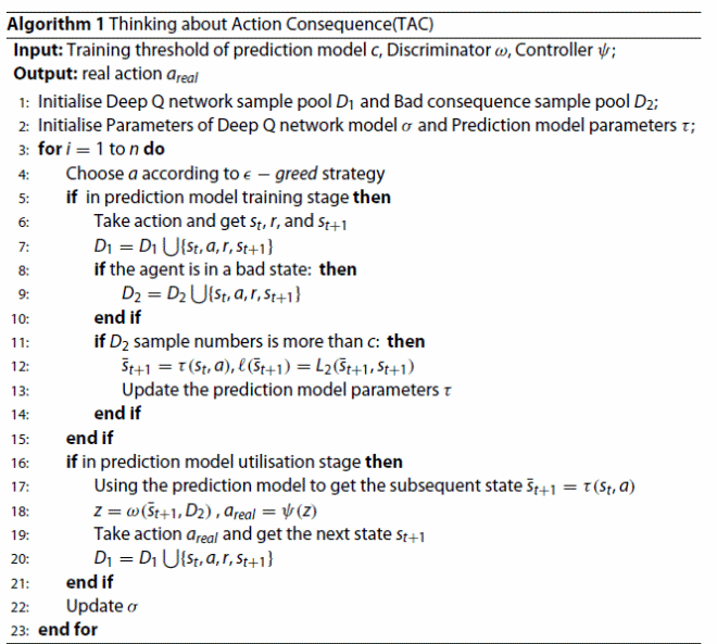
TAC divides the samples of the agent into experience replay buffer $D_1$ and the experience replay buffer of bad consequence $D_2$. The experience replay buffer $D_1$ is defined as the experience playback pool for training in the standard deep Q network methods; the experience replay buffer of bad consequence $D_2$ is added to our method, which is mainly composed of bad state or the states closer to task failure, to take advantage of the bad states, rather than ignore them like in the conventional method, as the bad consequence sample is an important part of the environment information that can be used to improve the performance of the algorithm further. In the process of training, the data are extracted from the experience replay buffer $D_1$ and the experience replay buffer of bad consequence $D_2$. For the samples in the experience replay buffer of bad consequence $D_2$, random samples are selected for training, and gradient descent training is conducted through (5(5) $b_t=GRU(s_t,a_t)$(5) )–(7(7) $\ell =L_2({\overline{s}}_{t+1},s_{t+1})$(7) ). After the forward prediction model is trained to a certain stage, the forward prediction is carried out for each action that is not restricted by the exploration selection in the $ϵ-greed$ strategy. The current state and the action to be executed are put into the prediction framework network to generate the future state. The future state and the experience sample pool are put into the discriminator ω for comparison: (8) $z=\omega ({\overline{s}}_{t+1},D_2)$(8) where z = 0 means that the predicted state is desired and then the controller ψ chooses $ϵ-greedy$ exploration strategy to select action; z = 1 indicates that the predicted state is terrible, and the controller ψ negates the action chosen by the exploration strategy of $ϵ-greedy$ and then turns to explore other space or execute the action corresponding to the maximum Q value of the current state.

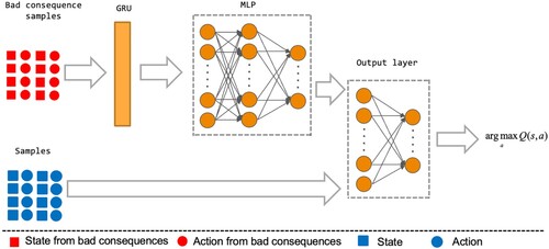
TAC can be equipped with many DRL algorithms, such as DQN, DDQN, DuDQN, and PerDQN. Figure 3 demonstrates the architecture of DRL with TAC.

Figure 3. Network structure. The TAC approach uses experience from bad consequences to improve the agent's actions.

4. Experimental settings

We used two different game environments, Box2d and Atari, and four different DRL algorithms to evaluate the method's performance. This section will introduce the environments and details of the setup.

Environment The game environment adopted in this study is mainly based on Box2d and Atari environment in Gym toolkit of Openai company. Table 2 shows the task name, number of actions, and introduction of the task. One environment, $Box2d$, adopts task “Lunarlander-v2”, where there are four candidate actions. As the agent may get a negative reward when it falls into traps, we collect the samples in the state of negative reward after executing the action as bad consequence samples. The other environment, Atari that mainly includes shooting games, sports competition games, action games, and so on, is different from the former. The agent gets a negative reward in a few games, most being zero or positive rewards. Thus, we define the bad consequence sample as the ones close to the failure in this case. In general, the bad consequence in the experiments of this study are defined as: (1) the state of executing actions and receiving negative rewards; (2) the countdown m states of agent's game failure; (3) the state composed of (1) and (2).

Table 2. A brief introduction to the game.

Task	Action	Agent task brief description
KungFuMaster	14	Agent need to defeat enemies on both sides
LunarLander	4	Agent need to learn to land and fly
Boxing	18	Agent need to defeat an enemy in the ring
Seaquest	18	Agent need to save lives in the sea

Training details In this study, we collect bad consequences from the environment as a pool of bad consequence samples and use a batch size of 32 each time. First, the hidden state is generated by GRU, and then the future state is output by MLP that consists of three fully connected networks that predict the future state through the input of belief state and action. For Atari environments, each state dimension is from 0 to 255, which is unsuitable as it significantly impacts the prediction accuracy. Therefore, we carried out normalisation by dividing the value with 255 so that the dimension of the state was adjusted to 0–1; the learning rate was set to 0.0005 to get a prediction network of bad states. Our algorithm uses predictive networks on the $ϵ-greedy$ strategy, which predicts the future picture of each exploration action and returns the results to the discriminator. The discriminator is mainly used to judge whether the action of executing the $ϵ-greedy$ is bad or not. The predicted future state is compared with the samples in the bad consequence pool using the mean square loss. If the mean square loss is greater than the threshold value, the action will have a bad consequence; if the calculated loss value is less than the threshold value, the action is considered a good one. The controller chooses whether to continue the exploration or other actions according to the returned results of the discriminator. If the discriminator's output is defined as profitable, it will continue to perform the action selected by the $ϵ-greedy$ policy. Otherwise, the action with maximum Q-value or the action of exploring other solution spaces will be chosen.

Baseline Our baseline methods are standard DQN, DDQN, Dueling DQN, and PerDQN, all using the $ϵ-greedy$ strategy for exploration. In the early stage, many random explorations are used to obtain sufficient environmental information. In the later stage, the collected environmental data is used to optimise the strategy. To ensure the experiment's reliability, we set the maximum experience pool of the four standard network methods as 100,000, extracting data from the experience sample pool each time. The batch size is 64, and the reward discount rate is 0.99.

Intrinsic reward We add an intrinsic reward constructed using uncertainty to the baseline. The uncertainty is mainly determined by the mean square error of the current state predicting the future state and the actual future state, allowing agents to have a curiosity mechanism and keep exploring the unknown space.

5. Results and analysis

In RL, the strategy is continuously optimised according to the cumulative reward defined as the criterion to judge the advantages and disadvantages of the RL algorithm. However, using deep learning to process images, some information loss and inaccurate results may be lost. Besides, some RL algorithms will adopt the $ϵ-greedy$ strategy, which further aggravates the volatility of the accumulated rewards of agents in the game process. Taking full consideration of these factors, it may not reflect the merits and demerits of the algorithm only by using the cumulative reward in a plot. Therefore, we use the average reward of games as the evaluation criterion of the algorithms, which can reduce the fluctuation of the test results and better reflect the advantages and disadvantages of the algorithm.

5.1. Experimental results

This subsection mainly introduces the comparison of our algorithm with the baseline and algorithms that incorporate Intrinsic Rewards(IR) in “LunarLander” of Box2D and “Boxing”, “KungFuMaster” and “Seaquest” in Atari.

Analysis of KungFuMaster In KungFuMaster, the agent observed the enemies on both sides and took action to defeat the enemies on both sides to gain points. Figure 4 demonstrated the comparisons of our algorithm with baseline algorithms and IR methods where the x-axis was the number of training plots, and the y-axis was the average cumulative reward.

Figure 4. Comparison of TAC with DQN and DQN-IR, DDQN and DDQN-IR, DuDQN and DuDQN-IR, PerDQN and PerDQN-IR in KungFuMaster.

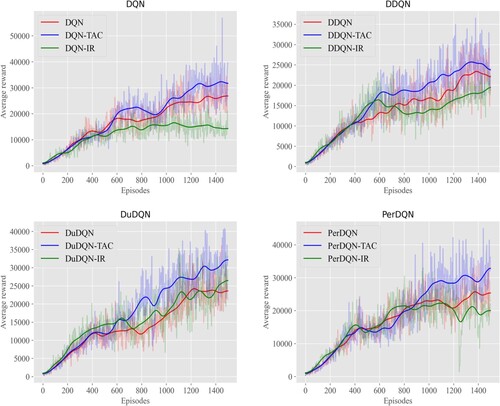
In KungFuMaster, agents could choose from 18 different actions, observe the enemies on both sides, and choose actions to fight the enemy to obtain points. If the agent was knocked down, the game would fail, which led to a slight difference between the bad state and the score state. It was difficult for the agent to distinguish the difference, leading to more dangerous traps ultimately. From Figure 4, it could be found that although the prediction was not accurate enough in the early stage for which the effect was not apparent, it shows good performance in the middle and late stages, while the IR method was even worse than the baseline. The main reason was that KungFuMaster's environment was complex. It was difficult to distinguish the bad state from the scoring state, which disturbed the original method by traps. However, the method added with the prediction framework could distinguish the bad state from the scoring state after continuous training. Therefore, in the middle and later stages, the intelligent experience could reduce the exploration of bad consequence space and explore other areas. As a result, the ability of the agent to score in the middle and late stages was significantly improved compared with the original method. Meanwhile, compared with the IR method, IR used intrinsic reward as reward shaping that further stimulated the exploration of unknown regions. But in more complex environments like KungFuMaster, agents needed to interact with the environment for a long time so that the IR method would converge more slowly.

Analysis of LunarLander In Lunarlander, agents could continuously obtain scores by learning to fly, and the agent could perform four actions to control the flight. Figure 5 demonstrated the comparisons of our algorithm with baseline algorithms and IR methods where the x-axis was the number of training plots, and the y-axis was the average cumulative reward.

Figure 5. Comparison of TAC with DQN and DQN-IR, DDQN and DDQN-IR, DuDQN and DuDQN-IR, PerDQN and PerDQN-IR in LunarLander.

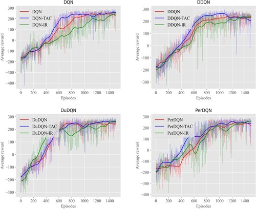
In Box2D, the state and action were relatively simple. Baseline algorithms had shown good performance to a certain extent, so our controller used the method of Q value to predict the bad state to escape from danger. As can be seen from Figure 5, compared with DQN, DDQN, PerDQN, because of the addition of prediction and judgment of bad state, the agent would not explore the bad consequence area too much in the early stage of the game, so that the agent will have higher scores in the early and middle stage of the game, and have similar performance in the convergence stage of the training. However, the effect of the DuDQN method with prediction framework was not noticeable, mainly due to the following two reasons: DuDQN algorithm itself had already had the judgment of the action influence; LunarLander environment was relatively simple, DuDQN had shown good performance in such environments. It could be found in Figure 5 that the performances of the baseline methods and the IR methods went up and down mutually in the early stage of the experiment but overlapped in the later stage. Because LunarLander was a simple environment, the area explored was relatively small, and the reward created by using uncertainty would decrease as the environment was better understood. The intrinsic reward would tend to be 0. Therefore, the effect was closer to baseline in the later stage.

Analysis of Boxing Boxing was a kind of action boxing game in the arena to beat the enemy to improve points. Figure 6 demonstrated the comparisons of our algorithm with baseline algorithms and IR methods where the x-axis was the number of training plots, and the y-axis was the average cumulative reward.

Figure 6. Comparison of TAC with DQN and DQN-IR, DDQN and DDQN-IR, DuDQN and DuDQN-IR, PerDQN and PerDQN-IR in Boxing.

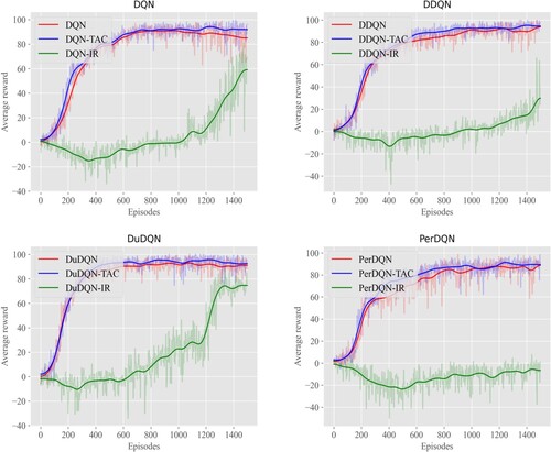
In the Boxing game, agents selected from 18 different actions to fight against the enemy. From Figure 6, it could be seen that the original DQN, DDQN, DuDQN, and PerDQN was relatively stable in the Boxing game, so this study adopted Q value to improve the controller. The main reason was that the original DQN, DDQN, DuDQN, and PerDQN had been more stable in the Boxing game and had a certain degree of stability. The ability to identify hazards was not significantly enhanced by adding the predictive framework approach. Still, it was also further enhanced to perform better than the original approach for almost any period. It could be concluded that although scores of IR methods were lower than those of the baseline methods, there was an upward trend in the end. The main reason was that there was some noise interference in the environment of Boxing, and according to Pathak et al. (2018) agents were quickly disturbed by the intrinsic rewards of uncertain manufacturing. Meanwhile, PerDQN is based on TD error for prioritising weighted samples for training, and the TD error of IR-based methods is more determined by uncertainty, which also leads to the low effect of PerDQN.

Analysis of Seaquest In the Seaquest, agents needed to dive into the sea to rescue people who were diving. During this period, they might encounter dangers from the seabed. Agents are required to avoid these dangers and save human beings. At the same time, they needed to send people to the sea for rescue. Figure 7 showed four different DRL algorithms (DQN, DDQN, DuDQN, PerDQN), IR methods, and TAC in the Seaquest game. The x-axis was the number of training scenarios, and the y-axis was the average cumulative reward.

Figure 7. Comparison of TAC with DQN and DQN-IR, DDQN and DDQN-IR, DuDQN and DuDQN-IR, PerDQN and PerDQN-IR in Seaquest.

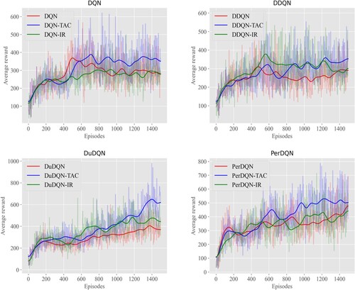
As shown in Figure 7, DQN, DDQN, DuDQN, and PerDQN were not evident in the early stages of Seaquest, but the method of adding prediction framework in the later stage was obviously improved. Especially in the DuDQN, the effect had been improved because the DuDQN method had a particular ability to judge the state and action. After the prediction framework method is added, the recognition ability of bad consequences was further strengthened. Therefore, the test results of DuDQN-TAC in Figure 7 were obviously beyond the original DuDQN method. As could be seen from the experimental results in Figure 7, the reward shaping method with uncertainty added was generally better than the baseline and even close to our TAC method in DDQN.

Limitations and utilisation Combining Table 3 with the experimental results, we can find that after adding the TAC method, for the relatively simple environment Lunarlander, there is only a certain effect in the middle of the training period. Still, for the latter training period, our method does not show a significant performance advantage. For the complex environment KungFuMaster, Seaquest in Atari, the introduction of the TAC method showed a relatively significant improvement. This is because, in these environments, the rules are complex, and the game gives more penalties and traps, so our method can identify a large number of future hazards and make strategic adjustments with a significant improvement over baseline. In environments such as Lunarlander, where the environment is simple, TAC can only identify risks and perform better in the middle of the game. Still, in the late game, traditional baselines can learn good strategies. Overall, with the introduction of the TAC method, it is challenging to be effective for algorithms with less exploration, and environments with simple environments and fewer penalties, especially in sparse rewards, may show lower performance. But for dense environments, especially in environments with more trap penalties, our method can improve the overall performance, especially in the later stages, and even exceed the original 50–100%, such as KungFuMaster. Besides, the prediction model framework was suitable for the above four algorithms and could improve the performance of some unrestricted random exploration RL algorithms. Meanwhile, the DRL method is one of the classical solutions for autonomous driving, but the safety issue is also an important constraint that checks and balances the development of the autonomous driving field. And the TAC method proposed in this paper, which uses prediction of subsumed consequences, has some implications for solving the safety problem in autonomous driving.

Table 3. DQN, DDQN,DuDQN,PerDQN, IR method and the TAC methods were compared for the last 200 episodes of the game.

Game		Baseline	with IR	with TAC
	DQN	265,41.0	147,36.5	313,00.5
KungFuMaster	DDQN	228,04.5	182,50.0	252,69.5
	DuDQN	234,35.5	237,70.0	304,21.5
	PerDQN	249,55.5	200,22.0	303,45.0
	DQN	241.9	219.6	252.1
LunarLander	DDQN	227.5	234.9	222.5
	DuDQN	239.5	245.2	261.0
	PerDQN	233.5	250.0	246.9
	DQN	86.4	45.8	92.0
Boxing	DDQN	90.7	17.8	94.4
	DuDQN	90.1	73.8	92.7
	PerDQN	86.5	−7.0	89.4
	DQN	289.9	284.6	361.3
Seaquest	DDQN	285.8	284.6	338.4
	DuDQN	382.6	452.2	620.1
	PerDQN	428.5	395.9	503.2

5.2. Comprehensive analysis

This subsection focussed on the average rewards for the 200 episodes in the middle and late stages and the whole experiment. Tables 3 and 4 showed the mean rewards in the middle and later stages of the experiment and throughout the experiment, respectively – Figures 8–9 show box plots for the corresponding data samples. According to Tables 3 and 4 and Figures 8–9, regarding DQN and DDQN, our method improved even in the KungFuMaster environment by 50–100% in all four environments than the conventional method and the IR method with the reward shaping. For DuDQN, our method was better than the traditional DuDQN and DuDQN-IR in all three environments, except in the middle and late stages of the simple environment LunarLander, i.e. the last two hundred episodes, but our method appeared to be more effective in terms of the average reward for the whole experiment. For PerDQN, although PerDQN-IR is better than PerDQN in specific environments, its performance is unstable and vulnerable to noise. Our method gains better performance compared with both PerDQN and PerDQN-IR.

Figure 8. Comparison of the box plots of the TAC method, the baseline, and the IR method for the last 200 episodes in KungFuMaster, LunarLander, Boxing and Seaquest.

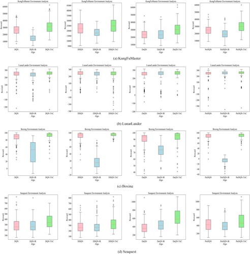
Figure 9. Comparison of the box plots of the TAC method, the baseline, and the IR method for the whole stage in KungFuMaster, LunarLander, Boxing and Seaquest.

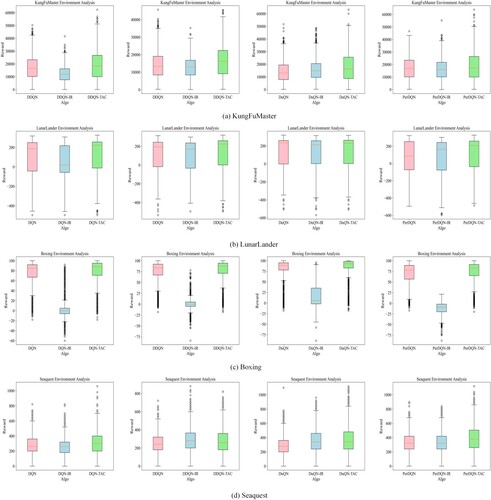
Table 4. DQN, DDQN,DuDQN,PerDQN, IR method and the TAC methods were compared for the entire stage.

Game		Baseline	with IR	with TAC
	DQN	169,93.9	121,95.9	189,92.3
KungFuMaster	DDQN	139,24.8	127,79.3	161,87.3
	DuDQN	140,33.5	154,96.1	178,15.7
	PerDQN	167,06.6	160,79.7	186,02.9
	DQN	103.2	60.2	126.5
LunarLander	DDQN	111.9	90.1	128.3
	DuDQN	136.1	135.2	138.9
	PerDQN	71.1	73.1	113.2
	DQN	73.1	4.0	76.4
Boxing	DDQN	73.0	0.2	76.0
	DuDQN	79.5	17.8	81.9
	PerDQN	68.0	−12.3	72.2
	DQN	283.1	262.8	310.7
Seaquest	DDQN	252.0	293.7	282.3
	DuDQN	291.9	352.9	377.8
	PerDQN	340.3	338.6	396.9

6. Conclusion

Since the DQN model represents the combination of deep learning and RL, this method combines the perception ability of deep learning with the decision-making of RL, which makes DRL enter into public view. However, DRL uses an unrestricted exploration strategy, which makes the agent ignore the existence of bad consequence spaces in the environment. Many agents explore bad consequence space, which will affect the observation of the overall environment. It means that taking into account changes in the environment, combining the environment with the current strategy, and continually avoiding possible bad consequence zones to improve the instant effect of each step to achieve the goal of maximum cumulative return. This study proposes the TAC method based on the prediction framework model to avoid random exploration of the bad state mentioned above. A forward prediction model sensitive to the future bad state is trained by using the sample pool of bad consequences by identifying the bad consequence samples. The future state is used to guide the current action selection, and the agent is separated from the danger, and the region's exploration has turned to safer areas. Although the TAC method in this paper mainly runs on game platforms such as Atari and Box2D, it is also highly relevant to autonomous driving because of its ability to improve the current action to escape from danger by predicting the consequences.

The experiment results show that the proposed TAC method with prediction framework has better scores at the same time due to the deviation from the average cumulative reward and reducing the exploration of bad consequence areas. At the same time, this study tests some games in Box2D and Atari environments, and the experimental results have been significantly improved, with certain generalisations.

Our TAC method, although improving strategies by predicting the consequences of actions, is more applicable in RL methods with a large amount of random exploration. Secondly, our method only performs one-step prediction and may lose prediction accuracy for predicting a more distant future. In the future, the prediction accuracy for the long term future (Ke et al., 2020) will be approached and combined with MPC to improve the performance of the algorithmic framework further.

Disclosure statement

The authors declare that the research was conducted in the absence of any commercial or financial relationships that could be construed as a potential conflict of interest.

Additional information

Funding

This work was supported by National Natural Science Foundation of China (61303108); Natural Science Foundation of Jiangsu Province (BK20211102); Suzhou Key Industries Technological Innovation-Prospective Applied Research Project (SYG201804); A Project Funded by the Priority Academic Program Development of Jiangsu Higher Education Institutions.

References

- Abed-alguni, B. H., & Ottom, M. A. (2018). Double delayed Q-learning. International Journal of Artificial Intelligence, 16(2), 41–59.
- Arulkumaran, K., Deisenroth, M. P., Brundage, M., & Bharath, A. A. (2017). Deep reinforcement learning: A brief survey. IEEE Signal Processing Magazine, 34(6), 26–38. https://doi.org/10.1109/MSP.2017.2743240
- Azar, M. G., Piot, B., Pires, B. A., Grill, J. B., Altché, F., & Munos, R. (2019). World discovery models (pp. 1–18). Preprint.
- Burda, Y., Edwards, H., Pathak, D., Storkey, A., Darrell, T., & Efros, A. A. (2018). Large-scale study of curiosity-driven learning. In Seventh international conference on learning representations (pp. 1–17). Proceeding of ICML.
- Ermolov, A., & Sebe, N. (2020). Latent world models for intrinsically motivated exploration. In Neural information processing systems (pp. 5565–5575). MIT Press.
- Feng, M., & Xu, H. (2017). Deep reinforecement learning based optimal defense for cyber-physical system in presence of unknown cyber-attack. In IEEE symposium series on computational intelligence (SSCI) (pp. 1–8). The Institute of Electrical and Electronics Engineers (IEEE).
- Frank, M., Leitner, J., Stollenga, M., Förster, A., & Schmidhuber, J. (2014). Curiosity driven reinforcement learning for motion planning on humanoids. Frontiers in Neurorobotics, 7(25), 1–15. https://doi.org/10.3389/fnbot.2013.00025
- Fujimoto, S., Hoof, H., & Meger, D. (2018). Addressing function approximation error in actor-critic methods. In International conference on machine learning (Vol. 80, pp. 1587–1596). ACM.
- Gangwani, T., Lehman, J., Liu, Q., & Peng, J. (2019). Learning belief representations for imitation learning in POMDPs. In Conference on uncertainty in artificial intelligence (pp. 1061–1071). AUAI Press.
- Gidaris, S., Singh, P., & Komodakis, N. (2018). Unsupervised representation learning by predicting image rotations. In International conference on learning representations (pp. 1–16). Proceeding of ICML.
- Goyal, P., Niekum, S., & Mooney, R. J. (2019). Using natural language for reward shaping in reinforcement learning. In International joint conference on artificial intelligence (pp. 2385–2391). AAAI Press.
- Gregor, K., Danihelka, I., Rezende, D., & Wierstra, D. (2015). Draw: A recurrent neural network for image generation. In Computer ENCE (pp. 1462–1471). Microtome Publishing.
- Haarnoja, T., Zhou, A., Abbeel, P., & Levine, S. (2018). Soft actor-critic: Off-policy maximum entropy deep reinforcement learning with a stochastic actor. In International conference on learning representations (pp. 1856–1865). Proceeding of ICML.
- Haber, N., Mrowca, D., Wang, S., Li, F. F., & Yamins, D. L. K. (2018). Learning to play with intrinsically-motivated self-aware agents. In Neural information processing systems (pp. 8388–8399). MIT Press.
- Hafner, D., Lillicrap, T., Fischer, L., Villegas, R., Ha, D., Lee, H., & Davidson, J. (2018). Learning latent dynamics for planning from pixels. In International conference on machine learning (pp. 2555–2565). Microtome Publishing.
- Hasselt, H. V., Guez, A., & Silver, D. (2016). Deep reinforcement learning with double q-learning. In Proceedings of the AAAI conference on artificial intelligence (Vol. 30, no. 1, pp. 1–7). The Institute of Electrical and Electronics Engineers (IEEE).
- He, K., Zhang, X. Y., Ren, S. Q., & Sun, J. (2016). Deep residual learning for image recognition. In IEEE conference on computer vision and pattern recognition (pp. 770–778). The Institute of Electrical and Electronics Engineers (IEEE).
- Henaff, M. (2019). Explicit explore-exploit algorithms in continuous state spaces. In Conference on neural information processing systems (pp. 9377–9387). MIT Press.
- Higgins, I., Pal, A., Rusu, A., Matthey, L., Burgess, C., Pritzel, A., Botvinick, M., Blundell, C., & Lerchner, A. (2017). Darla: Improving zero-shot transfer in reinforcement learning. In International conference on machine learning (pp. 1480–1490). Microtome Publishing.
- Katt, S., Oliehoek, F., & Amato, C. (2019). Bayesian reinforcement learning in factored POMDPs. In International conference on autonomous agents and multiagent systems (pp. 7–15). International Foundation for Autonomous Agents and Multiagent Systems.
- Ke, N. R., Singh, A., Touati, A., Goyal, A., Bengio, Y., Parikh, D., & Batra, D. (2020). Learning dynamics model in reinforcement learning by incorporating the long term future (1–14). Preprint.
- Lee, D., Seo, H., & Jung, M. W. (2012). Neural basis of reinforcement learning and decision making. Annual Review of Neuroscience, 35(1), 287–308. https://doi.org/10.1146/neuro.2012.35.issue-1
- Li, H. B., & Li, Z. S. (2018). A novel strategy of combining variable ordering heuristics for constraint satisfaction problems. IEEE Access, 6(1), 42750–42756. https://doi.org/10.1109/ACCESS.2018.2859618.
- Liang, Y. J., Xiao, M. Q., Wang, X. F., Tang, X. L., Zhu, H. Z., & Li, J. F. (2019). A POMDP-based optimization method for sequential diagnostic strategy with unreliable tests. IEEE Access, 7(1), 75389–75397. https://doi.org/10.1109/Access.6287639
- Lillicrap, T. P., Hun, J. J., Pritzel, A., Heess, N., Erez, T., Tassa, Y., Silver, D., & Daan, W. (2016). Continuous control with deep reinforcement learning. In International conference on learning representations (pp. 1–14). Proceeding of ICML.
- Lim, M. H., Tomlin, C. J., & Sunberg, Z. N. (2020). Sparse tree search optimality guarantees in POMDPs with continuous observation spaces. In International joint conference on artificial intelligence (pp. 4135–4142). AAAI Press.
- Marom, O., & Rosman, B. (2018). Belief reward shaping in reinforcement learning. In The association for the advance of artificial intelligence (pp. 3762–3769). AAAI Press.
- Mnih, V., Badia, A. P., Lillicrap, T., Harley, T., Silver, D., & Kavukcuoglu, K. (2016). Asynchronous methods for deep reinforcement learning. In International conference on machine learning (pp. 1928–1937). Microtome Publishing.
- Mnih, V., Kavukcuoglu, K., Silver, D., Graves, A., Antonoglou, I., Wierstra, D., & Riedmiller, M. (2013). Playing atari with deep reinforcement learning. In Neural information processing systems deep learning workshop (pp. 1–9). MIT Press.
- Moreno, P., Humplik, J., Papamakarios, G., Pires, B. Á., Buesing, L., Heess, N., & Weber, T. (2018). Neural belief states for partially observed domains. In NeurIPS 2018 workshop on reinforcement learning under partial observability (pp. 1–5). MIT Press.
- Nair, A., Pong, V., Dalal, M., Bahl, S., Lin, S., & Levine, S. (2018). Visual reinforcement learning with imagined goals. In Advances in neural information processing systems (pp. 9191–9200). MIT Press.
- Ostrovski, G., Bellemare, M. G., Oord, A., & Munos, R. (2017). Count-based exploration with neural density models. In International conference on machine learning (Vol. 70, pp. 2721–2730). Microtome Publishing.
- Pathak, D., Agrawal, P., Efros, A. A., & Darrell, T. (2018). Curiosity-driven exploration by self-supervised prediction. In International conference on machine learning (pp. 2778–2787). Microtome Publishing.
- Pathak, D., Gandhi, D., & Gupta, A. (2019). Self-supervised exploration via disagreement. In International conference on machine learning (pp. 5062–5071). Microtome Publishing.
- Schaul, T., Quan, J., Antonoglou, I., & Silver, D. (2016). Prioritized experience replay. In International conference on machine learning (pp. 1–21). Microtome Publishing.
- Sekar, R., Rybkin, O., Daniilidis, K., Abbeel, P., Hafner, D., & Pathak, D. (2020). Planning to explore via self-supervised world models. In International conference on machine (pp. 8583–8592). Microtome Publishing.
- Silver, D., Lever, G., Heess, N., Degris, T., Wierstra, D., & Riedmiller, M. (2014). Deterministic policy gradient algorithms. In International conference on machine learning (pp. 387–395). Microtome Publishing.
- Wang, R. W., Xia, W., Yap, R. H., & Li, Z. H. (2016). Optimizing simple tabular reduction with a bitwise representation. In International joint conference on artificial intelligence (pp. 787–793). AAAI Press.
- Wang, Z., Schaul, T., Hessel, M., Hasselt, H., Lanctot, M., & Freitas, N. (2016). Dueling network architectures for deep reinforcement learning. In International conference on machine learning (pp. 1995–2003). Microtome Publishing.
- Watkins, C., & Dayan, P. (1992). Q-learning. Machine Learning, 8(3–4), 279–292. https://doi.org/10.1007/BF00992698
- Xu, X., Zuo, L., & Huang, Z. H. (2014). Reinforcement learning algorithms with function approximation: Recent advances and applications. Information Sciences, 261(5), 1–31. https://doi.org/10.1016/j.ins.2013.08.037.
- Zhang, Z., Zhang, Y., Liu, G. C., Tang, J. H., Yan, S. C., & Wang, M. (2020). Joint label prediction based semi-supervised adaptive concept factorization for robust data representation. IEEE Transactions on Knowledge and Data Engineering, 32(5), 952–970. https://doi.org/10.1109/TKDE.69
- Zhang, Z. Z., Hsu, D., & Lee, W. S. (2014). Covering number for efficient heuristic-based POMDP planning. In International conference on machine learning (pp. 28–36). Microtome Publishing.
- Zhang, Z. Z., Hsu, D., Lee, W. S., Lim, Z. W., & Bai, A. (2015). Please: Palm leaf search for POMDPs with large observation spaces. In International conference on international conference on automated planning and scheduling (pp. 249–257). AAAI Press.