Hierarchical-fuzzy allocation and multi-parameter adjustment prediction for industrial loading optimisation

Abstract

Conventional manual-programmable logic controller systems have confronted the problems of the unbalance load and the unreasonable bins allocation in industrial loading field. Furthermore, various optimisation models with multi-agent systems have been proposed for the single-layer scheduling and communicating, which results in either a high time cost or a difficult multi-target regression. In this paper, we propose a hierarchical-fuzzy bins allocation method and a multi-parameter adjustment values prediction model in the multi-agent collaborative control system. The method intuitively achieves topgallant and hierarchical bins allocation by different fuzzy rule bases. The multi-parameter adjustment values prediction model utilising parallel-multi LSTM(PM-LSTM) is located on the accurate multi-parameter prediction. First, new loading reference standards and an abnormal data procession method are adopted for the dataset collection. Second, the LSTM-1 is used to extract the time-series features in the loading process. Third, a two-dimensional and reconstructed matrix integrates comprehensive features with the feature crossover method. The matrix will be used as inputs to predict the adjustment value of multi parameters by the LSTM-2. Finally, the relationship model among multi parameter values is built and fitted. Experiment results show better effects for the reasonable bins allocation and balanced industrial loading.

KEYWORDS:

• Parameters prediction
• industrial loading
• LSTM neural network
• hierarchical fuzzy calculation

1. Introduction

The manual-programmable logic controller system (MPLCs) provides some evident characteristics (i.e. anti-interference and high-reliability performance) convenient for workers (Jani et al., 2020; Krupa et al., 2021) while substantially increasing the possibility of manual intervention. It means that the referential operation metrics for daily loading control always rely on the manual experience, which has been applied in industrial material loading. The industrial loading field, aiming to achieve accurate and quantitative target loading, has attracted much attention from enterprises. However, the loading process based on MPLCs often suffers from the unbalanced load problem caused by the high error of various parameters (i.e. truck speed and belt conveyor flow) and requires reloading of the stopped truck. In addition, a real-time loading value is barely satisfied with selected bins pre-stored following a manual experience. Namely, the above problems will cause major losses and safety hazards to the enterprise. Hence, it is challenging to accurately reduce high errors of adjustment parameters to prevent unbalanced loading while making a reasonable bins allocation.

To the best of our knowledge, the related allocation issue can be solved with the target approximation. Che et al. (2020) propose a coordinated optimal operation strategy for generation optimisation and coal management. Qiao et al. (2020) present a novel partial repair rescheduling solution model to consider unexpected events and/or expanded performance criteria. However, the effective application results are only for discrete scenarios and single partial repair in the semiconductor system. Wang et al. (2021) propose a genetic algorithm-back propagation neural network method to achieve single-target evaluation and optimise the back propagation neural network. In a word, these methods mentioned above cannot be well fitted with the actual bins allocation problem and are short of the ability of multi-layer recursive calculation for parameters.

Additionally, the multi-agent system has recently become a significant focus of industrial research. However, the existing scheduling/communicating methods that rely on the single-layer neural network strategy in multi-agent systems difficult to achieve multi-target regression (Han et al., 2020; Liang et al., 2021; Zhao et al., 2020). Fortunately, we have found that the long short-term memory (LSTM) based on the advantage of long-time series prediction ability can solve multi-parameter's high error problems. For example, Srivastava et al. (2020) combine the convolution neural network with the LSTM to predict the power generated by wind turbines. Because the model composed of two layers processes the characteristic by characteristic in order, it cannot be well adapted to the multi-parameter feature matrix. Xue et al. (2021) utilise a prediction of pedestrian paths-LSTM model to improve the potential destinations’ prediction accuracy. Mackenzie et al. (2019), Mou et al. (2019) provide optimal and long short-term memory models for short-term prediction of traffic flows. These models directly predict data based on initial feature items and are unable to further explore the hidden relationship between the multi-parameter. Thus, two critical targets should be considered. (1) How to achieve a better-balanced loading via a multi-output neural network, while the predicted and applied parameters of the network can fit the loading standards (e.g. the absolute value of height error for each loading area is less than 0.15 m). (2) what should be considered to optimise the rationality of the bins allocation strategy.

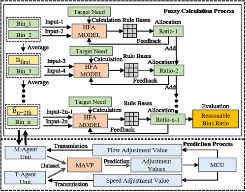
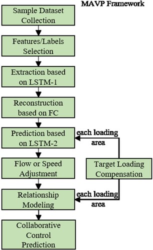
Based on the two considered objectives, we propose a hierarchical-fuzzy bin allocation (HFA) method and a multi-parameter adjustment values prediction (MAVP) model in the multi-agent collaborative control system (MACCs), which is shown in Figure 1. The HFA method is a hierarchical calculation method with different fuzzy rule bases, which is adopted for reasonable bins allocation. The MAVP model is used to collaborative control features extraction and accurate multi-parameter prediction. It is based on the parallel-multi long short-term memory (PM-LSTM) neural network and the feature crossover (FC) method. Further, the FC method is adopted to reconstruct extracted features to improve the multi-parameter prediction ability. The main contributions are summarised as follows.

1. The optimal strategy of material bins allocation on the hierarchical fuzzy calculation method. A novelty HFA method is proposed to actively obtain the topgallant and reasonable bins allocation ratio by different fuzzy rule bases in each fuzzy calculation layer.

2. The data procession process combines with the moment balance. The analysis of the moment balance for the objective carriage is to help to process abnormal data and to acquire the sample dataset. In addition, the related loading reference standards and deviation metrics are adopted to constrain the range of the sample dataset.

3. Accurate adjustment value prediction of multi parameters via parallel-multi deep learning model. The PM-LSTM for the MAVP model is adopted to solve the unbalanced loading problems. The parallel-multi neural network extracts the collaborative control features for its formidable extraction ability and accurately predicts the adjustment parameters based on regression characteristics for long-time series (He et al., 2019; Shu et al., 2021; Zhou & Xu, 2021). Further, the FC method expands the connection between hidden features as a two-dimensional reconstructed matrix to improve the feature extraction accuracy.

4. Multi parameters’ relationship model building and fitting based on neural networks. A relationship model among the parameters (i.e. the adjustment value of the truck speed and the flow of the belt conveyor) predicted by the MAVP model and target loading compensation is reasoned and built. The model aims to provide advanced adjustment values as a kind of reference. Further, we applied the model to the parameters’ adjusting in collaborative control of the industrial loading field.

Figure 1. The structure of the multi-agent collaborative control system.

The remainder of this paper is organised as follows: Section 2 introduces relevant model structures of the MACCs. Section 3 presents the experimental results and some comparative analysis. Finally, the conclusion and future works are given in Section 4.

2. The model construction via neural network and fuzzy allocation method

This section will introduce the optimal bins allocation ratio method and the accurate multi-parameter parallel prediction model.

2.1. The optimal bins allocation based on HFA method

Hierarchical fuzzy control is a kind of fuzzy control strategy that uses multiple fuzzy controllers of multi-input to accurately estimate the target value. It has been widely applied in the approximate logic coupling of the uncertain models (Sun & Huo, 2016; Yu et al., 2021). The hierarchical fuzzy calculation strategy can synthesise practical problems well to obtain the best results. Motivated by the idea, we propose a hierarchical-fuzzy bins allocation method for the material bins allocation optimisation. The method includes three critical steps: First, the allocation ratio of two random bins that considers the different kinds of fuzzy rulesets is obtained in the initial layer, shown in Figure 2. Second, both the average value of bins in the previous layer and the value of the new-selected bin will be added to calculate a relative allocation ratio in the next layer. Finally, according to the evaluation formula, the reasonable allocation ratio of all bins can be acquired in the final layer.

Figure 2. The process of bins allocation ratio in the initial layer.

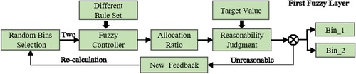
2.1.1. Bins allocation in initial fuzzy calculation layer

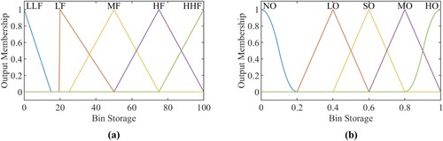
In this paper, let $B=(b_1,b_2,\dots ,b_n)$ denotes the carriage's quantified storage value of each material bin, where $n(n\ge 4)$ is the number of the material bins, $b_1,b_2,\dots ,b_n\in (0,100]$. In the initial allocation layer, we randomly select two bins $b_1$ and $b_2$ as the allocation input objects. The fuzzy sets of inputs and the outputs are virtually characterised by their membership functions. The degree of membership functions is shown in Figure 3(a), which is adopted to determine the degree of the membership (e.g. 1 denotes the highest degree, 0 denotes the lowest degree of membership). Figure 3(b) shows the outputs’ membership functions (i.e. three-trimf, one-smf, and one-zmf functions). Among them, the inputs’ membership functions are represented by five linguistic descriptions: low-low flag (LLF), low flag (LF), medium flag (MF), high flag (HF), high-high flag (HHF). Similarly, the outputs’ MFs include five linguistic descriptions: zero output (NO), low output (LO), small output (SO), medium output (MO), high output (HO).

Figure 3. (a) The MFs diagram of inputs (b) The MFs diagram of outputs.

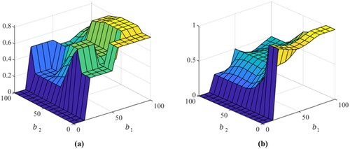
In the first layer, the domain of inputs and outputs are designed as [0,100] and [0,1] respectively, and the fuzzy rule bases in the first layer are described as $D_0=(d_1,d_2,\dots ,d_i)$, $i$ is the number of the fuzzy rule bases. The fuzzy rule base ($d_i$) is created for different bins allocation strategies. The surfaces of fuzzy rule bases are shown in Figure 4(a) and 4(b). Based on the above fuzzy rule bases, the general form of a fuzzy allocation rule is given as follows:

If $b_1$ is $A_j$ and $b_2$ is $A_k$, then $x_1$ is $C_l$ and $x_2$ is $C_m$

where $A_j$ and $A_k$ denote the discrete fuzzy sets of bin sets ($b_1$ and $b_2$), and $C_l$, $C_m$ denote the different and fuzzy bin allocation ratio, $C\in (0,1)$, which belongs to the fuzzy rule base $d_i$. For instance: if $b_1$ is LF and $b_2$ is MF, then $x_1$ is LO and $x_2$ is MO.

Figure 4. The fuzzy rule bases of the first layer.

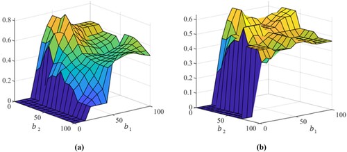
The allocation ratios of the bins based on the different kinds of fuzzy rule bases can be described as $X_{first}(X_1,X_2,\dots ,X_i)$, which is shown in Formula 1. If each bin satisfies $M_T\ast X_i\le b_i,i\in [1,n]$, the bins allocation ratio $X_i$ will be selected as an element of the objective output in the first layer. Further, the average value (${\overline{b}}_1$), being used as an input to improve the bins allocation rationality and accuracy in the second layer, is shown in Formula 2. (1) $\begin{array}{rl}& X_i\ast M_T\subseteq \{x_1\ast M_T\le b_1\cap x_2\ast M_T\le b_2\},0\le X_i\le 1\\ & \Rightarrow {X^{\mathrm{\prime }}}_{first}(X_1,X_2,\dots ,X_{\phi }),\phi \le i\end{array}$(1) (2) $\begin{array}{rl}& {\overline{b}}_1\text{ = average}(b_1,b_2),{\overline{b}}_1\in (0,100)\end{array}$(2) where the $X_{first}^{\mathrm{\prime }}(X_1,X_2,\dots ,X_{\phi })$ denotes the selected allocation ratios in the first layer (e.g. $X_1=(0.45,0.55)$ means that the allocation ratio of $b_1$ and $b_2$ are 0.45 and 0.55, respectively). $M_T$ is the loading target value. $\text{average}(\cdot )$ is the average function for each layer. The constraint of the first layer is $\{x_1\ast M_T\le b_1\cap x_2\ast M_T\le b_2,|{\sum }_{i=1}^2(x_i\ast M_T)-M_T|\le 0.5\}$.

2.1.2. Bins allocation in other fuzzy calculation layers

The relevant inputs’ MFs in next each layer are the same as membership functions in the first layer. However, the outputs’ membership functions include seven linguistic descriptions: high-high allocation, high allocation, little-high allocation, medium allocation, low allocation, low-low allocation, none allocation, which is remarked as {1, 0.8, 0.6, 0.5, 0.4, 0.2, 0}. The fuzzy rule bases in each layer are described as $D=(d_1^{\mathrm{\prime }},d_2^{\mathrm{\prime }},\dots ,d_i^{\mathrm{\prime }})$.

In the second layer, we let ${\overline{b}}_1$ and the new-added bin $b_3$ as the inputs for the fuzzy calculation. The surface views of each fuzzy rule base (e.g. $d_1^{\mathrm{\prime }}$, $d_2^{\mathrm{\prime }}$) are shown in Figure 5(a) and (b), and the general form of a fuzzy allocation rule is given as follows:

If $b_3$ is $A_j$ and ${\overline{b}}_1$ is $A_k$, then $X_{first}^{\mathrm{\prime }}$ is $E_l$ and $x_3$ is $E_m$

where $A_j,A_k$ denote the input fuzzy sets of the fuzzy rule base, $j,k$ is the number of the input fuzzy set. $E_l$, $E_m$ denote the discrete fuzzy output of different fuzzy rule bases, and $E_l,E_m\in d_i^{\mathrm{\prime }}$, $l,m$ is the number of the discrete output fuzzy set. $x_3$ is the allocation ratio of the bin $b_3$. For instance, if $b_3$ is HF and ${\overline{b}}_1$ is MF, then $X_{first}^{\mathrm{\prime }}$ is 0.8 and $x_3$ is 0.2.

Figure 5. The fuzzy rule bases of the second layer.

Based on the Formula (1) and (2) in the first fuzzy calculation layer, we can get the outputs of the second layer, which is shown as follows: (3) $\begin{array}{rl}& {X^{\mathrm{\prime }}}_{\sec ond}(X_1({X^{\mathrm{\prime }}}_{first},x_3),X_2({X^{\mathrm{\prime }}}_{first},x_3),\dots ,X_{\phi 2}({X^{\mathrm{\prime }}}_{first},x_3)),\phi 2\le i^2\cap x_3\ast M_T\le b_3,0\le X_i\le 1\\ & \Rightarrow (x_1,x_2,x_3{)}_{\sec ond}={X^{\mathrm{\prime }}}_{\sec ond}({X^{\mathrm{\prime }}}_{first}),{X^{\mathrm{\prime }}}_{\sec ond}(x_3)\end{array}$(3) (4) ${\overline{b}}_2\text{ = average}({\overline{b}}_1,b_3)$(4) where $X_{\sec ond}^{\mathrm{\prime }}(\cdot )$ denotes the objective output of the selected allocation set in the second layer. $\phi 2$ is the number of reasonable allocation ratio schemes in the second fuzzy calculation layer. $X_{\phi 2}(X_{first}^{\mathrm{\prime }},x_3)$ is an allocation ratio of $(b_1,b_2)$ and $b_3$. ${\overline{b}}_2$ is the average value of ${\overline{b}}_1$ and $b_3$. $X_{\sec ond}^{\mathrm{\prime }}(X_{first}^{\mathrm{\prime }})$ is the multiolicative allocation ratio of the second layer. The constraint of the second layer is {$x_3\ast M_T\le b_3,{\overline{b}}_2>0,|{\sum }_{i=1}^3(x_i\ast M_T)-M_T|\le 0.5$}.

Assumption 2.1:

It is assumed that the $(n-2)th$ outputs with inputs $({\overline{b}}_{n-3},b_{n\text{ - }1})$ and fuzzy rule base $d_i^{\mathrm{\prime }}\in D$ can be described as follows: (6) $\begin{array}{rl}& {\overline{b}}_{n-2}\text{ = average}({\overline{b}}_{n-3},b_{n-1})\end{array}$(6) (7) $\begin{array}{rl}& {X^{\mathrm{\prime }}}_{(n-2)th}(X_1({X^{\mathrm{\prime }}}_{(n-3)th},x_n),X_2({X^{\mathrm{\prime }}}_{(n-3)th},x_n),\dots ,X_{\phi (n-2)}({X^{\mathrm{\prime }}}_{(n-3)th},x_n))\\ & \phi (n-2)\le i^{n-2}\cap x_{n-1}\ast M_T\le b_{n-1},0\le X_i\le 1\end{array}$(7) (8) $\begin{array}{rl}& (x_1,x_2,x_{n-1}{)}_{(n-2)th}=X_{(n-2)th}^{\mathrm{\prime }}(X_{(n-3)th}^{\mathrm{\prime }}),X_{(n-2)th}^{\mathrm{\prime }}(x_{n-1})\end{array}$(8) where ${\overline{b}}_{n-2}$ is the average of ${\overline{b}}_{n-3}$ and $b_{n-1}$, $X_{(n-2)th}^{\mathrm{\prime }}$ denotes the objective output of the selected allocation set in $(n-2)th$ layer, and $(x_1,x_2,x_{n-1}{)}_{(n-2)th}$ is a simple expression form of the $X_{(n-2)th}^{\mathrm{\prime }}(\cdot )$. The constraint of the $(n-2)th$ layer is {$x_{n-1}\ast M_T\le b_{n-1},{\overline{b}}_{n-2}>0,|{\sum }_{i=1}^{n-1}(x_i\ast M_T)-M_T|\le 0.5$}.

Corollary 2.1:

Under the condition of Assumption, the objective output of the last layer can be obtained with $d_i^{\mathrm{\prime }}\in D$ and the $(n-1)th$ /last layer inputs ${\overline{b}}_{n-2}$,$b_n$, which is as follows: (9) $\begin{array}{rl}& {X^{\mathrm{\prime }}}_{(n-1)th}(X_1({X^{\mathrm{\prime }}}_{(n-2)th},x_n),X_2({X^{\mathrm{\prime }}}_{(n-2)th},x_n),\dots ,X_{\phi (n-1)}({X^{\mathrm{\prime }}}_{(n-2)th},x_n))\\ & \phi (n-1)\le i^{n-1}\cap x_n\ast M_T\le b_n,0\le X_i\le 1\end{array}$(9) (10) $\begin{array}{rl}& (x_1,x_2,\dots ,x_n{)}_{(n-1)th}={X^{\mathrm{\prime }}}_{(n-1)th}({X^{\mathrm{\prime }}}_{(n-2)th}),{X^{\mathrm{\prime }}}_{(n-1)th}(x_n)\\ & \Rightarrow {X^{\mathrm{\prime }}}_{final}=\{{X^{\mathrm{\prime }}}_{final\mathrm{\_}1},{X^{\mathrm{\prime }}}_{final\mathrm{\_}2},\dots ,{X^{\mathrm{\prime }}}_{final\mathrm{\_}\phi (n-1)}\}\end{array}$(10) where $x_n$ is the allocation ratio of the bin $b_n$ in the last layer. $X_{(n-1)th}^{\mathrm{\prime }}(\cdot )$ denotes the outputs of the selected allocation dataset in $(n-1)th$ layer, and $\phi (n-1)$ is the number of reasonable allocation ratio schemes in $(n-1)th$ layer. $X_{\phi (n-1)th}^{\mathrm{\prime }}(X_{(n-2)th}^{\mathrm{\prime }},x_n)$ is the multiplicative allocation ratio of $(b_1,b_2,\dots ,b_{n-1})$ and $b_n$, under the basis of the calculation ratio in $(n-2)th$ layer. $(x_1,x_2,\dots ,x_n{)}_{(n-1)th}$ is the allocation ratio sets of all bins in $(n-1)th$ layer. $X_{final}^{\mathrm{\prime }}(\cdot )$ is a simple expression form of the final output set. The constraint of the $(n-1)th$ layer is {$x_n\ast M_T\le b_n,{\overline{b}}_{n-1}>0,|{\sum }_{i=1}^n(x_i\ast M_T)-M_T|\le 0.5$}.

Proof 1: Based on inductive synthesis, when$n=2$, $(x_1,x_2)=X_{first}^{\mathrm{\prime }}(x_1),X_{first}^{\mathrm{\prime }}(x_2)\Rightarrow X_{first}^{\mathrm{\prime }}(X_1,X_2)$. For convenience, we can easily get that the bins allocation output of the$(n-2)th$ layer satisfies the Formula (10). Thus, the uniform expression for each layer is shown in Formula (11). (11) $\begin{array}{rl}& (x_1,x_2,\dots ,x_n{)}_{(n-1)th}={X^{\mathrm{\prime }}}_{(n-1)th}(X_{(n-2)th}({X^{\mathrm{\prime }}}_{(n-3)th}),X_{(n-2)th}(x_{n-2})),{X^{\mathrm{\prime }}}_{(n-1)th}(x_n)\\ & \Rightarrow {X^{\mathrm{\prime }}}_{(n-1)th}({X^{\mathrm{\prime }}}_{(n-2)th}),{X^{\mathrm{\prime }}}_{(n-1)th}(x_n),n>1\end{array}$(11) The final allocation ratio set for bins allocation is expressed in Formula (12). It can be well evaluated and selected by the final evaluation formula. The evaluation formula of the final bins allocation is given in Formula (13). The final objective of bins allocation strategy is shown in Formula (14).

Here, the time complexity of the allocation process in the initial fuzzy calculation layer based on the different kinds of fuzzy rule bases $D_1$ is $O(i)$. Further, the time complexity of the process in the last layer is $O(i^{n-2})$. The total time complexity of the fuzzy bins allocation algorithm is$O(i^{n-2})$. (12) $\begin{array}{rl}& X_{final\mathrm{\_}u}^{\mathrm{\prime }}=(x_{final\mathrm{\_}b1},x_{final\mathrm{\_}b2},\dots ,x_{final\mathrm{\_}bn})\end{array}$(12) (13) $\begin{array}{rl}& Eval(X_{final\mathrm{\_}1}^{\mathrm{\prime }},X_{final\mathrm{\_}2}^{\mathrm{\prime }},\dots ,X_{final\mathrm{\_}\phi (n-1)}^{\mathrm{\prime }})=\sum _{I=1}^n(b_I\cdot x_{final\mathrm{\_}bI}),|\sum _{I=1}^n(b_I\cdot x_{final\mathrm{\_}bI})-M_T|\le 0.5\end{array}$(13) (14) $\begin{array}{rl}& Objective=lim[M_T-Max(\sum _{I=1}^n(b_I\cdot x_{final\mathrm{\_}bI}))]\to \epsilon =0\end{array}$(14) where $X_{final\mathrm{\_}u}^{\mathrm{\prime }}$ is a kind of bins allocation ratio of the allocation ratio set $X_{final}^{\mathrm{\prime }}$ in the last layer, and $Eval(\cdot )$ is the evaluation function of the bins allocation.

2.2. The accurate parallel prediction on MAVP model

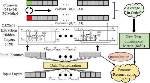
The long short-term memory can process and predict continuous time series with unknown sizes (Du et al., 2021; Wu et al., 2021). For the advantages, we propose a PM-LSTM neural network to achieve accurate parallel prediction. The framework includes three parts: sample dataset procession, multi-parameter adjustment value prediction via the PM-LSTM, and relationship model reasoning, which is shown in Figure 6.

Figure 6. The total framework of a parallel prediction model based on PM-LSTM.

2.2.1. Sample dataset procession

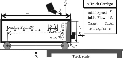
The industrial loading dataset usually has some high-error data because of discontinuous braking reload or parameters rough acquisition. To avoid adverse impacts and supplement the missing data of the raw dataset, we provide the new loading reference standards and an abnormal data procession method. The detailed process is described as follows:

1. Let $L_F$ represents the carriage wheelbase value, and $L_T$ is the carriage length. The target loading value is presented as $M_G$, the target loading time is $T_G$, the target loading height is $H_G$, and the empty carriage weight is $G_0$. The distance from each loading point to the rear wheel is $L_I$, $I\in [1,N-1]$, where $N$ denotes the number of loading points. $x_1,x_2,\dots ,x_{N-1}=L_F/(N-1)$ represent the distance between two adjacent loading points. In the first loading area, the initial truck speed and belt conveyor flow meet the Formula (15). The actual loading value is represented as $m_1$, and the target loading value is $m_1^{\mathrm{\prime }}=M_G/(n-1)$, so the error ($\mathrm{△}{m}_1$) between actual and the target is described in Formula (16) and (17): (15) $\begin{array}{rl}& \{\begin{array}{c}{V}_1=L_F/T_G\\ Q_1=M_G/T_G\end{array}\end{array}$(15) (16) $\begin{array}{rl}& m_1=\frac{2L_F{F}_1}{(L_F+L_T-x_1)\ast g}\end{array}$(16) (17) $\begin{array}{rl}& \mathrm{△}{m}_1={m_1}^{\mathrm{\prime }}-m_1\end{array}$(17) where $V_1$ denotes the initial truck speed and $Q_1$ denotes the initial belt conveyor flow. $F_1$ is the pressure value of the track scale in the first loading area. $g$ is 9.8 $m/s^2$.

2. Let $m_I^{\mathrm{\prime }}=m_1^{\mathrm{\prime }}+\mathrm{△}{m}_{I-1}$,$I>(1,N-1]$, denote the target loading value of the $I-th$ loading area. $\mathrm{△}{m}_{I-1}\text{ = }{m}_{I-1}^{\mathrm{\prime }}-m_{I-1}$ is the loading error between the actual and target value in $(I-1)-th$ loading area. The relative time consumption is $T_J,J\in [1,N-1]$, $F_I$ is the pressure value of the track scale in the $I-th$ loading area, and the material loading height of each area is denoted as $H_J,J\in [1,N-1]$. The schematic diagram for intuitive description is shown in Figure 7.

Figure 7. The schematic diagram of parameters.

Based on the calculation of the Formula (18) to (21), the sample dataset for relevant parallel LSTM model training is obtained, such that: (18) $\begin{array}{rl}& m_I=\frac{2(F_I-F_{I-1})L_F}{(L_F+L_T)-I{x}_I}\end{array}$(18) (19) $\begin{array}{rl}& \mathrm{\Delta }{m}_I=m_I^{\mathrm{\prime }}-m_I\end{array}$(19) (20) $\begin{array}{rl}& V_I=\frac{x_I}{T_I},Q_I=\frac{{m^{\mathrm{\prime }}}_I}{T_I}\end{array}$(20) (21) $\begin{array}{rl}& \mathrm{\Delta }{V}_I\text{ = }{V}_I-V_{I-1},\mathrm{\Delta }{Q}_I\text{ = }{Q}_I-Q_{I-1}\end{array}$(21) where $V_I$ denotes the truck speed and $Q_I$ denotes the belt conveyor flow in $I-th$ loading area. $\mathrm{\Delta }{V}_I$ and $\mathrm{\Delta }{Q}_i$ are the target adjustment value of the parameters for $I-th$ loading area.

2.2.2. Multi-parameter adjustment value prediction via the PM-LSTM

In this paper, the input data acquired by the above collection method contains seven features:

$S_{input}=[T,V,Q,H,m^{\mathrm{\prime }},m,\mathrm{△}m]$ (22)

1. To eliminate the adverse data effect and accelerate gradient descent, we adopt a data normalisation method based on the Z-Score function. Further, we process the input features using the following procedure, which can be formulated as: (23) $S_{input}^{\mathrm{\prime }}=\frac{(S_{input}-{\overline{S}}_{input})}{\delta }$(23) where ${\overline{S}}_{input}$ is the average value of the sample dataset, $S_{input}^{\mathrm{\prime }}$ denotes the normalised dataset, and $\delta$ is the standard deviation of the dataset.

2. The PM-LSTM model includes an input layer, an extraction hidden layer (LSTM-1), an inference hidden layer (LSTM-2), three fully connected layers, and an output layer. Considering the repetitive sub-unit structure of the LSTM, the single-cell contains several gates (i.e. input gate, forget gate, and output gate) to track the time-series information (Çınar & Tuncer, 2021; Zhang, Yu, et al., 2021). The relative formulas of statue information updates are described in Formula (24). (24) $\{\begin{array}{c}{f}_t=\sigma (W_f\cdot [h_{t-1},x_k^t]+b_f)\\ i_t=\sigma (W_i\cdot [h_{t-1},x_k^t]+b_i)\\ c_t=f_t{c}_{t-1}+i_t\tanh (W_c{x}_k^t+W_f{h}_{t-1}+b_c)\\ o_t=\sigma (W_o\cdot [h_{t-1},x_k^t]+b_o)\\ h_t=o_t\tanh (c_t)\end{array}$(24) where $f_t$ is the forgetting door, $i_t$ is the input gate, $c_t$ is the cell state at the time $t$, $o_t$ is the output gate, $h_t$ is the weight coefficient matrix, $b$ is the offset number, and $W_f$,$W_i$,$W_c$ are the training parameter, $\sigma$ is the activation function, $\tanh$ is the activation function.

3. Based on the time-series data processing capability of the LSTM-1 (Zhang, Yu, et al., 2021), the extracted features of multi-parameter (i.e. $Features-v$ and$Features-q$) are obtained. Furthermore, to explore further and synthesise the extracted features of the feature matrix extracted by the LSTM-1, the FC method is proposed in Formula (25). The FC method can average the hidden relationship and quantify the characteristics among different multi-adjustment parameters. It is based on the order sub-element crossover and value averaging of the changed feature vector. In addition, the detailed process of feature extraction by the FC method is shown in Figure 8. First, single element crossover in two feature vectors is used to change the original feature relationship. Second, the new hidden characteristics among the different parameters are acquired, which calculates the average value of the feature vector as the sub-element of the reconstructed vectors. Third, the new two-dimensional matrix of the multi-parameter features can be obtained by the sequential exchange and averaging operation. Namely, we calculate the average values of each new column vector as the relative elements and reshape as a restructuring multi-parameter extraction matrix. The shape of the new two-dimensional matrix is set to 64*2. Finally, we combine the initial features and the two-dimensional matrix as a feature reconstruction matrix. The shape of the feature reconstruction matrix is 71*2, which is expressed in Formula (26). (25) $\begin{array}{rl}& {\lambda }_{feature-v,i}\iff {\lambda }_{feature-q,i},i\in [1,64]\\ & \Rightarrow averag{e}_v(Features-v({\lambda }_{feature-q,i})),averag{e}_q(Features-q({\lambda }_{feature-v,i}))\\ & \Rightarrow (S_{input-v,1},S_{input-v,2},\dots ,S_{input-v,64}),(S_{input-q,1},S_{input-q,2},\dots ,S_{input-q,64})\\ & \Rightarrow (S_{input-v},S_{input-q})\end{array}$(25) (26) $\begin{array}{rl}& S_V=[S_{input}^{\mathrm{\prime }},S_{input-v}],S_Q=[S_{input}^{\mathrm{\prime }},S_{input-q}]\end{array}$(26) where $\lambda$ is the element of the feature matrix extracted by the LSTM-1. $S_{input-v}$ and $S_{input-q}$ are the input matrix of the LSTM-2, which are used to predict the adjustment value of the multi parameters.

   The LSTM-2 is adopted to parallelly predict the adjustment values of multi-parameter, which is based on the reconstructed features with the FC method. Namely, the LSTM-2 uses the 71 feature elements in the first matrix row to predict the adjustment values of the speed parameter. The other features in the second matrix row is for the adjustment values of the flow parameter. Further, we adopt two general dense layers to reduce the data dimension. Also, we convert the data dimension to obtain the predicted outputs parallelly. The related prediction principle can also be described in Formula (24). The output of the model is described in Formula (27). (27) $S_{output}=[\mathrm{\Delta }{V}_I^{\mathrm{\prime }},\mathrm{\Delta }{Q}_I^{\mathrm{\prime }}]$(27) where $\mathrm{\Delta }{V}_I^{\mathrm{\prime }}$, and $\mathrm{\Delta }{Q}_I^{\mathrm{\prime }}$ denote the predicted adjustment value of the truck speed and belt conveyor flow, respectively.

4. We use the Parallel Root Mean Square Error (PRMSE) to evaluate the proposed model. The evaluation metric measures the accuracy by the subtle deviation, which is defined as follows: (28) $PRMSE=\frac{1}{2}(\sqrt{\frac{1}{R}\sum _{z=1}^R{(S_z^V-S_z^{\mathrm{\prime }V})}^2}+\sqrt{\frac{1}{R}\sum _{z=1}^R{(S_z^Q-S_z^{\mathrm{\prime }Q})}^2})$(28) where $R$ denotes the number of the dataset instances. $S_z^V$ and $S_z^{\mathrm{\prime }V}$ represent the actual and predicted adjustment value of speed parameter with $z-th$ instance, respectively. $S_z^Q$ and $S_z^{\mathrm{\prime }Q}$ are the actual and predicted adjustment value of the flow parameter.

2.2.3. Relationship model derivation

Let $\mathrm{\Delta }m$ denotes the target loading compensation of each loading area, the truck speed adjustment value is $\mathrm{\Delta }{V}^{\mathrm{\prime }}$, and the adjustment value of belt conveyor flow is $\mathrm{\Delta }{Q}^{\mathrm{\prime }}$. The relationship among the $\mathrm{\Delta }{V}^{\mathrm{\prime }}$, $\mathrm{\Delta }{Q}^{\mathrm{\prime }}$, and $\mathrm{\Delta }m/dt$ presents a spatial linear relationship. When the relative parameters meet the condition of $\mathrm{\Delta }{V}^{\mathrm{\prime }}\ne 0$ and $\mathrm{\Delta }{Q}^{\mathrm{\prime }}\ne 0$, the relationship among these parameters can be described in Formula (29). Through the analysis of the time units for ($\mathrm{\Delta }{V}^{\mathrm{\prime }}\mathrm{\Delta }{Q}^{\mathrm{\prime }}$), we can find that the relationship among the flow adjustment value, the speed adjustment value, and the time interval can be expressed as $(\mathrm{\Delta }{V}^{\mathrm{\prime }}\mathrm{\Delta }{Q}^{\mathrm{\prime }})\propto t$. Thus, we assume the time cost of each relative loading area satisfies $t=\mu \cdot (\mathrm{\Delta }{Q}^{\mathrm{\prime }}\mathrm{\Delta }{V}^{\mathrm{\prime }})$, $\mu$ is a constant, the formula is shown in Formula (30). The final model expression is shown in Formula (31). (29) $\begin{array}{rl}& \frac{d\mathrm{\Delta }m}{dt}=\frac{d\mathrm{\Delta }m}{d(\mu \cdot (\mathrm{\Delta }{Q}^{\mathrm{\prime }}\mathrm{\Delta }{V}^{\mathrm{\prime }}))}\text{ = }\zeta (\alpha \cdot \mathrm{\Delta }{Q}^{\mathrm{\prime }}+\beta \mathrm{\Delta }{V}^{\mathrm{\prime }}),(\mathrm{\Delta }{Q}^{\mathrm{\prime }}\ne 0\mathrm{\&}\mathrm{\Delta }{V}^{\mathrm{\prime }}\ne 0)\end{array}$(29) (30) $\begin{array}{rl}\mathrm{\Delta }m& =\int \int \mu \cdot \zeta (\alpha \cdot \mathrm{\Delta }{Q}^{\mathrm{\prime }}+\beta \mathrm{\Delta }{V}^{\mathrm{\prime }})d\mathrm{\Delta }{Q}^{\mathrm{\prime }}d\mathrm{\Delta }{V}^{\mathrm{\prime }}\\ & \Rightarrow =\int \int (\mu \cdot \zeta \cdot \alpha \cdot \mathrm{\Delta }{Q}^{\mathrm{\prime }})d\mathrm{\Delta }{Q}^{\mathrm{\prime }}d\mathrm{\Delta }{V}^{\mathrm{\prime }}+\int \int (\mu \cdot \zeta \cdot \beta \cdot \mathrm{\Delta }{V}^{\mathrm{\prime }})d\mathrm{\Delta }{Q}^{\mathrm{\prime }}d\mathrm{\Delta }{V}^{\mathrm{\prime }}\\ & \Rightarrow \mathrm{\Delta }m=(\frac{\mu \cdot \zeta \cdot \alpha }{2}\text{)(}\mathrm{\Delta }{Q}^{\mathrm{\prime }}{\text{)}}^2(\mathrm{\Delta }{V}^{\mathrm{\prime }})+\text{(}\frac{\mu \cdot \zeta \cdot \beta }{2}\text{)(}\mathrm{\Delta }{Q}^{\mathrm{\prime }}\text{)}(\mathrm{\Delta }{V}^{\mathrm{\prime }}{)}^2\text{ + }{\rho }_3\end{array}$(30) (31) $\begin{array}{rl}& \mathrm{\Delta }m\text{ = }{\rho }_1\ast (\mathrm{\Delta }{Q}^{\mathrm{\prime }}{\text{)}}^2(\mathrm{\Delta }{V}^{\mathrm{\prime }})+{\rho }_2\ast \text{(}\mathrm{\Delta }{Q}^{\mathrm{\prime }}\text{)}(\mathrm{\Delta }{V}^{\mathrm{\prime }}{)}^2\text{ + }{\rho }_3\end{array}$(31) where $\zeta$ denotes a spatial coefficient, $\alpha$, $\beta$ are the two-dimensional plane coefficients, ${\rho }_1\text{ = (}\mu \cdot \zeta \cdot \alpha \text{)/2}$, ${\rho }_2\text{ = (}\mu \cdot \zeta \cdot \beta \text{)/2}$, ${\rho }_3$ are constant coefficients. In addition, we adopt the prediction values via the PM-LSTM to fit the parameters ${\rho }_1$, ${\rho }_2$, ${\rho }_3$. Namely, the correctness of the model inference derivation can be verified by whether the real values can be calculated. Among them, we need to consider the relationship between coordination parameters under special conditions. when$\mathrm{\Delta }{V}^{\mathrm{\prime }}\ne 0$,$\mathrm{\Delta }{Q}^{\mathrm{\prime }}\text{ = }0$, the time cost only depend on the speed parameter, we can assume that the relationship between speed adjustment value with the time cost satisfies $t=\mu \cdot (\mathrm{\Delta }{V}^{\mathrm{\prime }})$. Thus, the relationship formula can be described in Formula (32). Similarly, when$\mathrm{\Delta }{V}^{\mathrm{\prime }}=0$,$\mathrm{\Delta }{Q}^{\mathrm{\prime }}\ne 0$, and the time cost satisfies $t=\mu \cdot (\mathrm{\Delta }{Q}^{\mathrm{\prime }})$, the relationship formula can be described in Formula (33). Further, we will verify the hypothesis by the Experiment 2. (32) $\begin{array}{rl}& \frac{d\mathrm{\Delta }m}{dt}=\frac{d\mathrm{\Delta }m}{d({\mu }^{\mathrm{\prime }}\cdot (\mathrm{\Delta }{V}^{\mathrm{\prime }}))}\text{ = }{\zeta }^{\mathrm{\prime }}({\beta }^{\mathrm{\prime }}\mathrm{\Delta }{V}^{\mathrm{\prime }}\text{ + }{\theta }_1)\\ & \Rightarrow \mathrm{\Delta }m={\rho }_4(\mathrm{\Delta }{V}^{\mathrm{\prime }}{)}^2\text{ + }{\rho }_5(\mathrm{\Delta }{V}^{\mathrm{\prime }})\text{ + }{\rho }_6\end{array}$(32) (33) $\begin{array}{rl}& \mathrm{\Delta }m={\rho }_7(\mathrm{\Delta }{Q}^{\mathrm{\prime }}{)}^2\text{ + }{\rho }_8(\mathrm{\Delta }{Q}^{\mathrm{\prime }})\text{ + }{\rho }_9\end{array}$(33) where ${\theta }_1$ is a constant related to $\mathrm{\Delta }{V}^{\mathrm{\prime }}$. ${\rho }_4=(({\mu }^{\mathrm{\prime }}\cdot {\zeta }^{\mathrm{\prime }}\cdot {\beta }^{\mathrm{\prime }})/2)$, ${\rho }_5=(({\mu }^{\mathrm{\prime }}\cdot {\zeta }^{\mathrm{\prime }}\cdot {\theta }_1)/2)$, ${\rho }_6$, ${\rho }_7$, ${\rho }_8$, ${\rho }_9$ are constant coefficients which need to be calculated by the prediction values.

Figure 8. The diagram of the features extraction process.

3. Experiments

3.1. Experiment 1: the material bins allocation method comparison

In this experiment, the relevant training dataset of daily bins allocation is collected from the Huaibei Coal Mine Co. Ltd in Anhui Province, China. To ensure the effectiveness of comparison, we use the same dataset for model training and fuzzy rule bases design, which comes from the daily bins allocation process. We compare the HFA model with the GA-BPNN (Wang et al., 2021), GA-SVR (Ji et al., 2021), and GA-LSTM (Kara, 2021) to verify the allocation effect. The number of bins is 4. The parameters of the proposed HFA method are as follows: The number of fuzzy rule bases in the first layer is 9. The number of the fuzzy rule bases in other layers is 6. The number of fuzzy rules in each base is 100. The weight of fuzzy rules is 1. The connection method of elements in rules is “and”. We select 100 data with different bin storages as the test dataset. The parameters of each neural model are listed in Table 1.

Table 1. Parameters setting of each neural network model.

Model	Initial scale	Max generation	Mutation rate	Mutation scale	Crossover rate
GA	50	200	0.16	100	0.4
Model	Learning Rate	Network Layer	Neurons Number	Epochs	Kernel
BPNN	0.01	4	5/50/10/4	500	–
SVR	–	3	5/100/4	Tol<1*e^−3	RBF Kernel
LSTM	0.01	4	5/128/64/4	500	–

where $R^2=1-{\sum }_{i=1}^m{(y_i-{y^{\mathrm{\prime }}}_i)}^2/{\sum }_{i=1}^m{(y_i-\overline{y})}^2$ is the regression coefficient, $\overline{y}=({\sum }_{i=1}^m{y}_i)/m$, $MAE=({\sum }_{i=1}^m|y_i-{y^{\mathrm{\prime }}}_i|)/m$ is the mean absolute error, $RMSE=\sqrt{({\sum }_{i=1}^m{(y_i-{y^{\mathrm{\prime }}}_i)}^2)/m}$ is the root mean square error, $y_i$ is the target sum value of all bins, $y_i^{\mathrm{\prime }}$ is the predictive calculation value, $\overline{y}$ is the average calculation value.

Table 2 indicates that the evaluation metrics of our proposed method are better than that of other models, the R² value is about 0.932, the prediction loss of the proposed model is lowest (RMSE: 1.107, and MAE: 0.763). Table 3 shows that our proposed-HFA can accurately achieve the target value while ensuring that the allocation of each bin is reasonable. The predicted calculation value can get 69.90 t. Namely, the material bins allocation can be well optimised in the industrial loading process. Further, the bins allocation value of each model with fixed storage value is shown in Table 4, which calculates for the different target values. The sum of calculation of the HFA method is highest among all listed models (i.e. HFA vs GA-BPNN: 1.035; HFA vs GA-SVR: 1.052; HFA vs GA-LSTM: 1.019).

Table 2. Comparison metrics results of all contrast models.

Model	RMSE	MAE	R^2
GA-BPNN	1.543	1.355	0.919
GA-SVR	2.074	1.661	0.891
GA-LSTM	1.214	0.887	0.925
Proposed-HFA	1.107	0.763	0.932

Table 3. Comparison results with the target value (70 ton) and different bins storage value.

Model	$b_1$/ratio/storage	$b_2$ /ratio/ storage	$b_3$ /ratio/ storage	$b_4$ /ratio/ storage	Calculation value (t)	Consumption time (s)
Proposed-HFA	10.16 /0.145/30	4.71 /0.067/10	24.47/0.349/60	30.59/0.437/90	69.93	4.13
GA-BPNN	15.27/0.221/30	3.21 /0.047/10	13.26/0.192/60	37.24/0.540/90	68.98	7.65
GA-SVR	14.35/0.213/30	3.82/0.057/10	12.56/0.187/60	36.54/0.543/90	67.27	6.62
GA-LSTM	15.18/0.220/30	4.22/0.061/10	14.59/0.211/60	35.16/0.508/90	69.15	5.87
Proposed-HFA	12.50 /0.179/40	12.45 /0.178/40	22.65/0.253/40	22.35/0.247/40	69.95	4.34
GA-BPNN	12.97/0.185/40	21.15 /0.302/40	9.16/0.131/40	25.84/0.369/40	69.12	6.87
GA-SVR	12.49/0.184/40	20.61/0.305/40	10.16/0.151/40	24.36/0.360/40	67.62	7.02
GA-LSTM	12.48/0.180/40	21.36/0.308/40	10.42/0.150/40	25.18/0.363/40	69.44	5.41
Proposed-HFA	8.84 /0.126/50	8.87 /0.127/60	22.76/0.325/80	29.41/0.420/90	69.88	4.29
GA-BPNN	5.49/0.078/50	12.62 /0.180/60	22.96/0.328/80	28.17/0.402/90	69.24	6.56
GA-SVR	5.75/0.084/50	12.83/0.187/60	21.92/0.319/80	28.15/0.410/90	68.65	6.93
GA-LSTM	5.92/0.085/50	12.96/0.186/60	22.82/0.328/80	27.87/0.401/90	69.57	5.33

Table 4. Detail bins allocation value with fixed storage value for the different target value.

Methods	The HFA allocation method					The GA-BPNN allocation method
Target(t)	$b_1$(30)	$b_2$(50)	$b_3$(70)	$b_4$(80)	Sum(t)	$b_1$(30)	$b_2$(50)	$b_3$(70)	$b_4$(80)	Sum(t)
50	3.18	12.23	13.87	20.65	49.93	9.62	14.24	10.47	12.31	46.64
55	5.56	11.86	19.44	17.82	54.68	8.41	12.67	11.34	20.62	53.04
60	7.61	12.85	22.19	16.32	58.97	4.77	10.86	16.37	26.25	58.25
65	2.20	22.41	19.27	21.03	64.91	4.03	12.82	19.28	25.99	62.12
70	2.15	15.74	24.41	27.65	69.95	3.35	14.67	21.35	29.62	68.99
Methods	The GA-SVR allocation method					The GA-LSTM allocation method
Target(t)	$b_1$(30)	$b_2$(50)	$b_3$(70)	$b_4$(80)	Sum(t)	$b_1$(30)	$b_2$(50)	$b_3$(70)	$b_4$(80)	Sum(t)
50	9.84	10.26	11.77	13.39	45.26	10.19	15.19	9.88	13.49	48.72
55	8.92	13.71	10.03	19.17	51.83	9.17	12.89	10.11	21.34	53.51
60	5.02	8.64	15.79	27.72	57.17	5.17	9.67	16.52	27.13	58.49
65	4.26	13.62	17.33	26.84	62.05	4.43	13.07	18.61	26.76	62.87
70	3.76	16.38	19.65	28.47	68.26	3.86	16.23	20.77	28.42	69.28

3.2. Experiment 2: the accurate prediction effect of MAVP model

In this experiment, we take the 70(t)-capacity-carriage of the truck as the research object. The relative loading data collected from May 1st, 2020 to Dec 1st, 2020 are employed to run simulations. The loading reference standards are used to select the training dataset. The sample dataset selection standards for relevant parameters are shown in Table 5.

Table 5. The carriage parameters and dataset selection standards.

Standards	Definition	Value
Loading error	${\sum }_{i=1}^{118}{m}_i-M_G$	$\pm 1.50$ t
Loading Height-error	$H-H_G(2.8m)$	$\pm 0.20$ m
Standard Loading Time	–	240 s
Loading Capacity	$m_i\in [m^{\mathrm{\prime }}\pm 0.100]$	0.593 t±0.100 t
Loading points of Truck	–	118
Target Loading Value	$M_G$	70 t

To verify the accuracy of the MAVP model based on PM-LSTM neural network, we use the Intel i7-8700 CPU, the NVIDIA GTX 1080ti, the 16GB of memory, and the training process runs in the Python 3.8 programming environment. The sample data is 20,000, the epoch value of the LSTM-1 is 500, the number of extractions hidden nodes is 128, the learning rate of the LSTM-1 is 0.001. The epoch value of the LSTM-2 is 1000, the batch size of the neural network is 50, the loss function in the PM-LSTM is MSE, the number of inference hidden nodes is 64/32, and the dropout value of the PM-LSTM is 0.2. The neuron numbers of the fully connected layers are 32/16/2. Figure 9(a) shows that all training loss-epoch curves with different initial learning rates for LSTM-2. Figure 9(b) is the Logarithmic curve fitting of Figure 9(a), which makes it smoother and intuitively reflects the average loss value of the training effect. Additionally, the results of the detailed comparison information are shown in Table 6.

Figure 9. (a) The results of training loss for each learning rate (b) The fitting curve of comparison results.

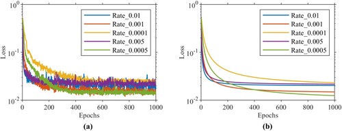
Table 6. The loss results of each initial learning rate for MAVP model.

Learning_rate	Training_Loss	Validation_Loss	PMSE
1e-2	0.0186	0.0239	0.0223
5e-3	0.0180	0.0228	0.0187
1e-3	0.0155	0.0177	0.0169
5e-4	0.0127	0.0142	0.0134
1e-4	0.0228	0.0284	0.0257

Figure 9(a) and (b) show that both curve convergence range and training precision value with the learning rate (5e-4) are superior to others. The downward trend curve in the early 200 epochs is obvious and inconsistent because the training dataset has different adaptability to the training process of each learning rate. Further, Table 6 provides the relevant loss value of the final epoch.

In the paper, we built the relationship model with the learning rate 5e-4. The detail and schematic diagram of the relationship model among $\mathrm{\Delta }m$, $\mathrm{\Delta }{V}^{\mathrm{\prime }}$, and $\mathrm{\Delta }{Q}^{\mathrm{\prime }}$ are shown in Figure 10 (a) and (b). To calculate the assumption parameter values in Formula 32 and 33, we fit the relationship model with the prediction data of the MAVP model. Thus, the function of the relationship model among the multi-parameter and the target loading compensation in Figure 10(a) is expressed as follows: $\mathrm{\Delta }m\text{ = }-1.47\ast {10}^7\ast (\mathrm{\Delta }{Q}^{\mathrm{\prime }}{\text{)}}^2(\mathrm{\Delta }{V}^{\mathrm{\prime }})+4.83\ast {10}^8\ast \text{(}\mathrm{\Delta }{Q}^{\mathrm{\prime }}\text{)}(\mathrm{\Delta }{V}^{\mathrm{\prime }}{)}^2\text{ + }2.4\ast {10}^{-4}$where boundary conditions satisfy as follows: when$\mathrm{\Delta }{V}^{\mathrm{\prime }}=0$ and $\mathrm{\Delta }{Q}^{\mathrm{\prime }}\ne 0$, $\mathrm{\Delta }m\text{ = }-\text{4}\text{.203}\ast {10}^5\ast (\mathrm{\Delta }{Q}^{\mathrm{\prime }}{\text{)}}^2-69.852\ast \text{(}\mathrm{\Delta }{Q}^{\mathrm{\prime }}\text{)}-0.0395$, and when $\mathrm{\Delta }{V}^{\mathrm{\prime }}\ne 0$ and $\mathrm{\Delta }{Q}^{\mathrm{\prime }}=0$, $\mathrm{\Delta }m\text{ = }-\text{2}\text{.041}\ast {10}^7\ast (\mathrm{\Delta }{Q}^{\mathrm{\prime }}{\text{)}}^2\text{ + }1.297\ast {10}^4\ast \text{(}\mathrm{\Delta }{Q}^{\mathrm{\prime }}\text{)}-0.776$.

Figure 10. (a) The diagram of the relationship model-1 (b) The diagram of the relationship model-2.

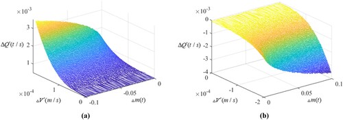
Concurrently, the function of the relationship model in Figure 10(b) is expressed as follows: $\mathrm{\Delta }m\text{ = }-1.52\ast {10}^7\ast (\mathrm{\Delta }{Q}^{\mathrm{\prime }}{\text{)}}^2(\mathrm{\Delta }{V}^{\mathrm{\prime }})+4.76\ast {10}^8\ast \text{(}\mathrm{\Delta }{Q}^{\mathrm{\prime }}\text{)}(\mathrm{\Delta }{V}^{\mathrm{\prime }}{)}^2-3.7\ast {10}^{-4}$where boundary conditions satisfy as follows: when $\mathrm{\Delta }{V}^{\mathrm{\prime }}=0$ and $\mathrm{\Delta }{Q}^{\mathrm{\prime }}\ne 0$, $\mathrm{\Delta }m\text{ = }-\text{3}\text{.109}\ast {10}^7\ast (\mathrm{\Delta }{Q}^{\mathrm{\prime }}{\text{)}}^2\text{ + }5.318\ast {10}^3\ast \text{(}\mathrm{\Delta }{Q}^{\mathrm{\prime }}\text{)}-0.0164$, and when $\mathrm{\Delta }{V}^{\mathrm{\prime }}\ne 0$ and $\mathrm{\Delta }{Q}^{\mathrm{\prime }}=0$, $\mathrm{\Delta }m\text{ = }1.054\ast {10}^7\ast (\mathrm{\Delta }{Q}^{\mathrm{\prime }}{\text{)}}^2\text{ + }2.087\ast {10}^3\ast \text{(}\mathrm{\Delta }{Q}^{\mathrm{\prime }}\text{) + }0.134$.

3.3. Application results

In this paper, we apply the above-provided relationship model via the PM-LSTM in the MACCs and compare it with the conventional MPLC system to verify the superior performance in industrial loading. The primary configuration in the Huaibei coal mine is listed in Table 7, and actual loading diagrams of the system are shown in Figure 11 (a) and (b).

Figure 11. (a) The diagram of the system console (b) The diagram of loading monitoring parameters.

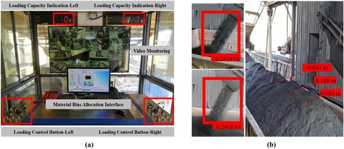
Table 7. The major configuration of the industrial loading.

Device	Model	Number	Unit	Origin
Master console	LYZK-2	2	set	Jiangsu
Control cabinet	ILNS-200	2	station	Jiangsu
Wheeled distance collector	LCD-2-3	2	station	Jiangsu
Vehicle position recogniser	PZ-M51P	2	set	Jiangsu
Wheel detector	LYL-G-1	8	set	Jiangsu
Vehicle number recognition device	LYJRF34A	2	set	Jiangsu
Coal falling sensor	LYMW-2W	20	set	Jiangsu
PLC cabinet	SELF MADE	2	set	Anhui
Explosion-proof motor	YBBP-4-55	2	station	Anhui

Based on the above configuration, we collected the material loading data of the selected 50 carriages from Jan 1st, 2021 to Jan 31th, 2021. The average metrics (i.e. actual material load, time consumption) of each carriage are shown in Figure 12 (a) and (b). Table 8 shows the load variance and average capacity of each loading group. The results indicate that all carriages’ material loading effect is nearly 69 t, and the average time consumption of the loading process is close to 235 s. It means that the industrial loading process based on the MACCs can get good performance.

Figure 12. (a)  The effect of actual material loading (b) The effect of actual time consumption.

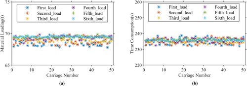
Table 8. The variance and mean value of actual material loading and time consumption in each group.

	Actual material load(t)			Actual time consumption(s)
Group	Variance (σ)	Average (υ)	Group	Variance (σ)	Average (υ)
1	0.3042	68.8788	1	3.6087	234.5263
2	0.2146	69.02824	2	3.2507	235.0765
3	0.1086	69.1019	3	1.9396	235.1256
4	0.0528	69.4011	4	1.1247	235.2778
5	0.0112	69.4566	5	0.5264	235.2541
6	0.0104	69.4559	6	0.4891	235.2289

The historical data of the carriage (i.e. No.1653599) from Dec 1st, 2020 to Dec 31th, 2020 is collected from the coal mine. The comparison results of actual loading based on the MAVP model and conventional MPLC system are shown in Figure 13. The MACC system outperforms the conventional MPLC system, and the actual material loading capacity based on the MACCs is more stable and accurate, about 69.4 t. The time consumption is about 230 s, which is significantly less than the contrast system.

Figure 13. (a) The actual loading comparison results of systems (b) The loading time consumption results of systems.

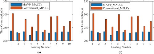
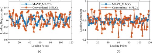
Figure 14(a) and (b) show that the comparison results of loading height error and loading capacity in a continuous process. The loading height-error and loading capacity of the MACCs for each loading area satisfy the indicators in Table 3 (i.e. Area Loading Height-error and Area Loading Capacity). Namely, the loading capacity of each loading point belongs to [0.493, 0.693 t], and the absolute value of the loading height-error is less than 0.2 m. Namely, the optimised industrial loading based on MACCs has a good effect. In addition, the material loading balance compared with the conventional MPLCs is increased (i.e. absolute average height-error: 0.092 m vs 0.169 m, the standard deviation of loading capacity: 0.057 t vs 0.113 t).

Figure 14. (a) Height errors of each loading point (b) Capacity errors of each loading point.

3.4. Discussion and analysis

In this paper, the discussion and analysis of the experimental and applicational results are as follows:

1. The HFA method indicates better bins allocation ability for industrial loading. Because the fuzzy toolbox has a strong logic inference and calculation ability, we can use our proposed HFA method to optimise the bins allocation ratio and reduce allocation time consumption. The hierarchical fuzzy allocation guarantees the accuracy of the target loading value, and the evaluation formula further selects the most reasonable bins allocation ratio. The reason is that the different kinds of fuzzy rule bases in each layer can promote the fuzzy approximation target value within the allowance range. During the fuzzy calculation process in each layer, adding a single bin at a time can simplify the logic or time complexity.

2. The MAVP model based on PM-LSTM and FC method can further achieve regression accuracy and robustness for the long time series. Because of the memory cell accumulator and formidable extraction ability, the forward neural network LSTM-1 can be adopted as a feature extractor to sequence inputs. It means that the LSTM extracts subsequent features of the sequence and selectively merges them with the initial time features (Duguma et al., 2021;  Zhang, Zhang, et al., 2021). With the help of the FC method, the hidden and comprehensive relationship among the adjustment parameters can be described as a two-dimensional feature matrix. Due to the method orderly adopting the average feature value substitution to integrate and reconstruct the multi-parameter independent features, the LSTM-2 can predict the multi-target parameters with low loss value.

3. The relationship among target loading compensation and multi parameters can be well fitted. Based on the theoretical derivation and proof of the relationship model, we can get the collaborative relationship between the adjustment values of multi-parameter and the target compensation value, which is first mentioned in the industrial loading field. Because of the high-precision prediction of adjustment parameters via the MAVP model, the relationship model's coefficients can be accurately calculated.

4. Conclusion

This paper proposes a HFA method and the MAVP model applied in the MACCs for optimising the bins allocation ratio and achieving accurate parameters prediction. In addition, the relationship model among the target loading compensation and adjustment values of multi parameters are derived and well built. Experimental and applicational results demonstrate that the MACCs can significantly solve the industrial loading problems of conventional MPLCs (i.e. unreasonable bin allocation strategy and dangerous eccentric load). It also can dramatically improve the loading efficiency and reduce the workload of the coal mining workers. However, the HFA method has the limitation in that the computational complexity of the strategy and the number of rule sets will suddenly increase with the increase of bins number. In the future, we will combine the resource scheduling algorithm with the HFA method to optimise computational consumption. Further, we want to explore the application of the more precisive MAVP model in the rail-mounted industrial loading field for collaborative control.

Disclosure statement

No potential conflict of interest was reported by the author(s).

Additional information

Funding

This work was supported by National Natural Science Foundation of China: [Grant Number No.51675003,No.51874010]; National key R&D project (intelligent dispatching technology for all mine personnel and materials): [Grant Number No.2020YFB1314103].

References

- Che, P., Liu, Y., Che, L., & Lang, J. (2020). Co-Optimization of generation Self-Scheduling and coal supply for Coal-Fired power plants. IEEE Access, 8, 110633–110642. https://doi.org/10.1109/access.2020.2989514
- Çınar, A., & Tuncer, S. A. (2021). Classification of normal sinus rhythm, abnormal arrhythmia and congestive heart failure ECG signals using LSTM and hybrid CNN-SVM deep neural networks. Computer Methods in Biomechanics and Biomedical Engineering, 24(2), 203–214. https://doi.org/10.1080/10255842.2020.1821192
- Du, J., Vong, C., & Chen, C. L. P. (2021). Novel efficient RNN and LSTM-like architectures: Recurrent and gated broad learning systems and their applications for text classification. IEEE Transactions on Cybernetics, 51(3), 1586–1597. https://doi.org/10.1109/TCYB.2020.2969705
- Duguma, D. G., Kim, J., Lee, S., Jho, N., Sharma, V., & You, I. (2021). A lightweight D2D security protocol with request-forecasting for next-generation mobile networks. Connection Science, 1–25. https://doi.org/10.1080/09540091.2021.2002812
- Han, Y., Li, C., Zhang, W., & Ahmad, H. G. (2020). Impulsive consensus of multiagent systems with limited bandwidth based on encoding–decoding. IEEE Transactions on Cybernetics, 50(1), 36–47. https://doi.org/10.1109/TCYB.2018.2863108
- He, Z., Zhou, Z., Gan, L., Huang, J., & Zeng, Y. (2019). Chinese entity attributes extraction based on bidirectional LSTM networks. International Journal of Computational Science and Engineering, 18(1), 65. https://doi.org/10.1504/IJCSE.2019.096988
- Jani, M., Garg, P., & Gupta, A. (2020). Performance analysis of a mixed cooperative PLC–VLC system for indoor communication systems. IEEE Systems Journal, 14(1), 469–476. https://doi.org/10.1109/JSYST.2019.2911717
- Ji, Y., Xu, K., Zeng, P., & Zhang, W. (2021). GA-SVR algorithm for improving forest above ground biomass estimation using SAR data. IEEE Journal of Selected Topics in Applied Earth Observations and Remote Sensing, 14, 6585–6595. https://doi.org/10.1109/JSTARS.2021.3089151
- Kara, A. (2021). Multi-step influenza outbreak forecasting using deep LSTM network and genetic algorithm. Expert Systems with Applications, 180, 115153. https://doi.org/10.1016/j.eswa.2021.115153
- Krupa, P., Limon, D., & Alamo, T. (2021). Implementation of model predictive control in programmable logic controllers. IEEE Transactions on Control Systems Technology, 29(3), 1117–1130. https://doi.org/10.1109/TCST.2020.2992959
- Liang, H., Liu, G., Zhang, H., & Huang, T. (2021). Neural-network-based event-triggered adaptive control of nonaffine nonlinear multiagent systems with dynamic uncertainties. IEEE Transactions on Neural Networks and Learning Systems, 32(5), 2239–2250. https://doi.org/10.1109/TNNLS.2020.3003950
- Mackenzie, J., Roddick, J. F., & Zito, R. (2019). An evaluation of HTM and LSTM for short-term arterial traffic flow prediction. IEEE Transactions on Intelligent Transportation Systems, 20(5), 1847–1857. https://doi.org/10.1109/TITS.2018.2843349
- Mou, L., Zhao, P., Xie, H., & Chen, Y. (2019). T-LSTM: A long short-term memory neural network enhanced by temporal information for traffic flow prediction. IEEE Access, 7, 98053–98060. https://doi.org/10.1109/ACCESS.2019.2929692
- Qiao, F., Ma, Y., Zhou, M., & Wu, Q. (2020). A novel rescheduling method for dynamic semiconductor manufacturing systems. IEEE Transactions on Systems, Man, and Cybernetics: Systems, 50(5), 1679–1689. https://doi.org/10.1109/TSMC.2017.2782009
- Shu, X., Zhang, L., Sun, Y., & Tang, J. (2021). Host–parasite: Graph LSTM-in-LSTM for group activity recognition. IEEE Transactions on Neural Networks and Learning Systems, 32(2), 663–674. https://doi.org/10.1109/TNNLS.2020.2978942
- Srivastava, T., Vedanshu, & Tripathi, M. M. (2020). Predictive analysis of RNN, GBM and LSTM network for short-term wind power forecasting. Journal of Statistics and Management Systems, 23(1), 33–47. https://doi.org/10.1080/09720510.2020.1723224
- Sun, L., & Huo, W. (2016). Adaptive fuzzy control of spacecraft proximity operations using hierarchical fuzzy systems. IEEE/ASME Transactions on Mechatronics, 21(3), 1629–1640. https://doi.org/10.1109/TMECH.2015.2494607
- Wang, L., Zhou, H., Yang, J., Xiong, Y., She, J., & Chen, W. (2021). A decision support system for tobacco cultivation measures based on BPNN and GA. Computers and Electronics in Agriculture, 181, 105928. https://doi.org/10.1016/j.compag.2020.105928
- Wu, S., Liu, Y., Zou, Z., & Weng, T. (2021). S_I_LSTM: Stock price prediction based on multiple data sources and sentiment analysis. Connection Science, 1–19. https://doi.org/10.1080/09540091.2021.1940101
- Xue, H., Huynh, D. Q., & Reynolds, M. (2021). PoPPL: Pedestrian trajectory prediction by LSTM with automatic route class clustering. IEEE Transactions on Neural Networks and Learning Systems, 32(1), 77–90. https://doi.org/10.1109/TNNLS.2020.2975837
- Yu, R., Chen, Y., Han, B., & Zhao, H. (2021). A hierarchical control design framework for fuzzy mechanical systems with high-order uncertainty bound. IEEE Transactions on Fuzzy Systems, 29(4), 820–832. https://doi.org/10.1109/TFUZZ.2020.2965913
- Zhang, S., Yu, H., & Zhu, G. (2021). An emotional classification method of Chinese short comment text based on electra. Connection Science, 1–20. https://doi.org/10.1080/09540091.2021.1985968
- Zhang, S., Zhang, Z., Chen, Z., Lin, S., & Xie, Z. (2021). A novel method of mental fatigue detection based on CNN and LSTM. International Journal of Computational Science and Engineering, 24(3), 290. https://doi.org/10.1504/IJCSE.2021.115656
- Zhao, Z., Liu, S., Zhou, M., Guo, X., & Qi, L. (2020). Decomposition method for new single-machine scheduling problems from steel production systems. IEEE Transactions on Automation Science and Engineering, 17(3), 1–12. https://doi.org/10.1109/TASE.2019.2953669
- Zhou, Z., & Xu, H. (2021). Large-scale multiagent system tracking control using mean field games. IEEE Transactions on Neural Networks and Learning Systems, 32(5), 1–9. https://doi.org/10.1109/TNNLS.2021.3071109