Using active learning selection approach for cross-project software defect prediction

Abstract

Cross-project defect prediction (CPDP) technology can effectively ensure software quality, which plays an important role in software engineering. When encountering a newly developed project with insufficient training data, CPDP can be used to build defect predictors using other projects. However, CPDP does not take into account the prior knowledge of the target items and the class imbalance in the source item data. In this paper, we design an active learning selection algorithm for cross-project defect prediction to alleviate the above problems. First, we use clustering and active learning algorithms to filter and label some representative data from the target items and use these data as prior knowledge to guide the selection of source items. Then, the active learning algorithm is used to filter representative data from the source items. Finally, the balanced cross-item dataset is constructed using the active learning algorithm, and the defect prediction model is built. In this article, we selected 10 open-source projects by using common defect prediction models, active learning algorithms, and common evaluation metrics. The results show that the proposed algorithm can effectively filter the data, solve the class imbalance problem in cross-project data, and improve the defect prediction performance.

KEYWORDS:

• Active learning
• cross-project
• software defect prediction
• transfer learning

1. Introduction

With the continuous advancement of science and technology, the use of software has spread in all walks of life and is closely related to life. Once there is a problem with the software, it will behave abnormally, and even bring about a catastrophic disaster in severe cases (Wong et al., 2010, 2017). Software defects are the direct cause of software problems. In the early stages of software development, we can use software defect prediction technology to lock down potential defect modules in advance, thereby reducing the impact of software defects (Li et al., 2019; Wong et al., 1998, 2000). Software defect prediction technology can build a software defect prediction model by mining historical warehouse information combined with machine learning and other methods. In this way, more resources are effectively applied to the defective modules, which effectively ensures the quality of the software.

At present, within-project defect prediction (WPDP) algorithms have attracted the attention of many researchers. Defect prediction models are built with machine learning methods (Kitchenham et al., 2007). In real-world scenarios, new development projects often encounter some problems, such as insufficient training data and high labelling costs (Menzies et al., 2010). Cross-project defect prediction (CPDP) has become an important research direction (Li et al., 2017). However, CPDP constructs defect classifiers by other items and does not take into account the prior knowledge of the target item and the defect patterns between the source and target items (He et al., 2012). Therefore, this paper uses an active learning algorithm to construct a priori knowledge from the target items to guide the selection of source items.

In this paper, we propose an algorithm for data filtering which uses the active learning selection approach for cross-project defect prediction (ALSA). In the first step, the target items are aggregated into multiple clusters by a clustering algorithm, from which representative data is filtered and manually annotated. In the second step, 20% of the data from the target items is screened and manually labelled by combining active learning algorithms, and the labelled data is used as prior knowledge. In the third step, data is screened from the source items based on prior knowledge, and then the screened data and prior knowledge are combined into an enhanced training set by data fusion, and a defect prediction model is constructed by the Naive Bayes method. In the fourth step, considering the class imbalance problem of the screened data, an active learning algorithm is used for data balancing (Kim et al., 2020).

In order to verify the effectiveness of the proposed method in this paper, we investigate the following questions:

1. How does the defect prediction performance of methods that use active learning for data filtering compare to methods that do not use data filtering? Which active learning method yields the best performance?

Effective training data is a strong guarantee for implementing defect predictors. The traditional method constructs a defect prediction model from source item data without considering the prior knowledge of the target item, which makes it difficult to match the defect pattern between the source item and the target item. The active selection method screens data from the source items based on the prior knowledge of the target items and combines prior knowledge to form an enhanced dataset. To answer this question, we use the CPDP approach without data filtering for comparison. Then, by comparing different active learning strategies, we try to find a strategy that allows the model to perform optimally.

1. There is still a class imbalance problem with the data filtered from the source project. How effective is it to use active learning methods to solve the problem? What is the optimal sampling rate?

When there is an imbalance in the data, the classification model will focus more on most categories of data, which will directly affect the performance of the model. Random undersampling is a classical method to solve the imbalance problem. However, the traditional random undersampling method may lead to the loss of data containing important information. Using active learning methods can retain the data with a high contribution and remove the data with a low contribution (Ge et al., 2020). To answer this question, this paper compares multiple imbalance methods and then tries to find an optimal balance ratio based on active learning algorithms.

1. Compared with traditional WPDP, how does the proposed method perform?

Turhan et al. (2013) pointed out that WPDP is the best method in the practice of software defect prediction, which can get ideal performance. Therefore, the effectiveness of the method in this paper can be verified by comparing the performance with WPDP.

To verify the validity of ALSA experiments, this paper is based on 10 open source projects. The final results show that the proposed method outperforms the CPDP method without data filtering, and the best performance can be obtained by using an uncertainty sampling strategy; the active balancing algorithm has better performance compared with the traditional methods for solving class imbalance, and the ALSA method can be a strong competitor to the WPDP method.

The main contribution of this paper is to change the traditional idea of passive data selection by using a priori knowledge combined with an active classifier to filter the data. Another contribution is the active balance method, which is an optimisation of the undersampling method and is suitable for solving imbalance problems. These methods will provide good guidance for the selection of source and target terms.

The rest of the paper is structured as follows. The second section introduces the background of cross-project software defect prediction technology and active learning technology; the third section introduces the ALSA method and details of the target project screening stage and the source project screening stage combined with pseudocode; and the fourth section concludes. The fourth section describes the experimental data, indicators, models, and settings, among other things. The fifth section presents and analyses the results of the experiment. The remaining chapters introduce the validity of the experiment, conclusions, and future work.

2. Background and related work

2.1. Cross-project defect prediction technology

In real-world scenarios, CPDP is a powerful solution to the lack of traditional data. A number of open source datasets for software defect prediction have been used for research. Due to the problem of data drift caused by various factors between projects, building the model directly from the source project cannot obtain better performance. Transfer learning is applied to fields with similar targets but different feature spaces and distributions. It can be compatible with more data and is widely used in image processing, natural language processing, and other fields.

In recent years, the research of transfer learning combined with cross-project defect prediction has become more and more abundant, which effectively alleviates a series of problems caused by data drift. In the field of software defect prediction, we can transfer the software defect knowledge learned from the source project to the target project space, which is beneficial to the construction of software defect prediction models. The existing research literature is divided into research based on feature transfer and research based on software module transfer.

The main idea of feature migration-based research is to make the source and target project data have similar distribution spaces and to maximise the retention of data features that conform to independent and identical distribution conditions. He et al. (2015) pointed out that the migration method based on feature selection is used to obtain software defect features that satisfy both source and target projects. In this way, the optimal feature subset can be obtained on the premise of preserving the data features. Then, combined with the machine learning classification algorithm, a cross-project software defect prediction model is built. In the process of pre-processing the source project, this paper adopts the migration method based on feature selection, which effectively utilises the software defect information in the source project and the target project.

The reference (Nam et al., 2013) adopts a feature map-based migration method, which minimises the distance by means of data distribution and maps the source item and the target item into the same space. When researchers found that changing the range of control features through pre-learning methods such as normalisation would have a certain impact on the model, they proposed the TCA+ method. The transfer method based on feature mapping is suitable for data that is quite different from the field, and usually conducts analysis and research on dimension reduction and mathematics. The reference (Cruz & Ochimizu, 2009) studies the features of both the source item and the target item at the same time through the feature transformation transfer method. The logarithmic transformation method is adopted to optimise the quality of the data and reduce the influence of noise in the data, thus improving the performance of the software defect prediction model.

Based on instance migration, the research idea is to migrate software module instances to modules with rich software defect information. The reference (Turhan et al., 2009) proposes the Burak filtering method, which uses the KNN algorithm to filter similar data from source items according to the target item. The Burak filtering method gets good performance, but only passively in the source item. It does not consider inter-data characteristics in the filtering process. According to the idea of the Burak algorithm, this paper uses information-rich data as prior knowledge to guide the selection of target and source items. The reference (Menzies et al., 2012) aggregates data into multiple clusters by clustering, and then selects data with high correlation as a unit to build a local software defect prediction model.

Traditional cross-project defect prediction uses feature transfer and software module transfer based methods to construct models. These approaches process the software data based on the distribution characteristics between the source and target projects, thus reducing the differences between projects. However, the CPDP does not take into account the priori knowledge of the target project and the imbalance of cross-project data.

2.2. Active learning technology

In recent years, massive amounts of data have been emerging, but the cost of manual annotation is expensive. How to reduce the cost of labelling has become a difficult problem. So active learning technology appeared in front of people’s eyes. Active learning has two functions. The first one is the filtering function. It can filter out the data with high contributions to the modality. The second is the annotation function. It can use labelled data to build a model to judge unlabelled data, and provide labels for unlabelled data. Traditional machine learning methods build models from labelled data, which is passive learning. Through active learning, the model can interact with the training data during the training process, actively select training samples, and provide timely feedback. Figure 1 shows the difference between active mode and passive mode.

Figure 1. Active mode and passive mode.

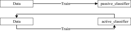
The process of active learning is as follows: The first step is to build a data pool. The data pool contains an initial label set L and an unlabelled set U. Usually, the initial label set needs to be manually labelled. In the second step, we build the model using the initial set of labels and then filter the data from the unlabelled set through an active learning strategy. The data filtered here is the data with the hightest contribution to the model. The third step is to add the filtered data to the initial label set L. The fourth step is to use the initial label set L for training. Iterate according to the above steps until the set conditions are met.

Common active learning strategies are as follows:

1. Uncertainty-based sampling strategy: This is the most widely used strategy to filter out the most uncertain data in a sample. Such data generally contains a large amount of information.

2. Committee-based query strategy: Similar to the ensemble learning algorithm, it can construct multiple classifiers from the current version to vote on and then select the data with the most votes. Such algorithms run slower.

3. Density-based sampling strategy: Such algorithms sample according to the density scale of the data and are not affected by the classifier (Zemmal et al., 2021).

In recent years, active learning has been applied to the field of software defect prediction. Most of them work within the project and can achieve better results. Lu et al. combined cross-version software defect prediction with active learning to achieve data augmentation between similar versions (2014). Yuan et al. (2020) combined cross-item defect prediction with active learning for the first time. He combines active learning with a feature map-based transfer learning approach. This method effectively solves the problems of large differences in data distribution and high labelling costs.

3. Method

In this chapter, the overall framework of the ALSA algorithm is first introduced, and then the target item and source item filtering methods are introduced in detail.

3.1. The framework of ALSA

The Figure 2 shows the overall flow of the algorithm.

Figure 2. The ALSA algorithm flow.

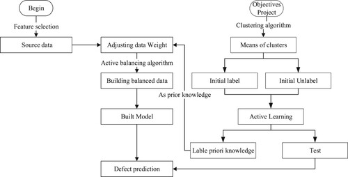
The ALSA algorithm consists of two phases: the target item selection phase and the source item selection phase. In the target item selection phase, in order to filter out the representative data in the target items, the K-medoids method is used to aggregate the data into multiple clusters and select the centre of each cluster for manual annotation (Xu et al., 2021). When the annotated data contains two categories, it is filtered and manually annotated from the target items in combination with the active learning method. In the source item selection phase, the annotated data in the target items is used as prior knowledge, and then filtered from the source items based on prior knowledge. Finally, the active learning algorithm is used to solve the imbalance problem of the selected data and construct the defect prediction model.

3.2. The details of ALSA

We describe the experimental procedure in Algorithm 1 and Algorithm 2.

1. Target project selection stage.

Table

Algorithm 1 Target project selection stage
Input:
Unlabeled data(U), the weights of the labeled data (α), the number cluster(β), Target data(T)
Output:
Labeled data
1:	label = NULL, unlabel = U
2:	CLUS1,CLUS2 = Kmedoids(T,β)
3:	prior = CLUS1 + CLUS2
4:	AL = active learning(prior)
5:	label = AL(unlabel, α)
6:	Label = label1∪label2
7:	Return Label

The target item selection algorithm is an algorithm that can filter data based on the characteristics between items. The algorithm can filter out the data with high contributions, label them, and finally get a certain number of labelled data sets. The algorithm uses a combination of clustering algorithms and active learning algorithms. The clustering algorithm is an unsupervised learning algorithm, so the clustering algorithm is used to select representative data from the target items.

The steps of the algorithm are as follows: First, the target items are aggregated into multiple clusters using the K-medoids algorithm, and then the cluster centre data is selected for manual annotation. When the labelled data contains both defective and non-defective items, a combination of active learning algorithms is used to select the target items. The active learning algorithm can construct active learners based on the labelled data, and then select samples with a high contribution from the unlabelled data and perform manual labelling. Finally, the labelled data is added to the initial labelled dataset and the next round of selection is performed (Bengar et al., 2021).

When the filtered data reaches α times the number of target items, the search is stopped and the final label set is obtained. According to (Xu et al., 2018), it is an acceptable cost range to control the number of data annotations within 20% of the total. In this experiment, we set α to 0.2.

1. source project selection stage

Table

Algorithm 2 Source project selection stage
Input:
Source data(S), Target data(T) source item filter data weight(u),
imbalance ratio l (l = majority/minority)
Output:
Training dataset
1:   S’ = feature transfer(S,T)
2:   AL = active learning(Lable)
3:   Which(weight = u and Imbalanceratio = l)
4:   Data[1, … ,n] = S[n]
5:   S'' = AL(S',u)
6:   R = rank(S'')
7:   Ddefect = Defect distinction (R)
8:   Dno_defect = Defect distinction (R) * I
9:   Train = Ddefect ∪Dno_defect
10:  Return Train

The source item selection algorithm is an algorithm that filters based on prior knowledge of target items. It can filter out the source project data with a high contribution according to the characteristics of the data and solve the imbalance problem in the data. Finally, it is combined with prior knowledge to form an enhanced data set to build a software defect prediction model (Bhosle & Kokare, 2020).

• In the first step, the characteristics of the source project and the target project are compared. Source item data for the same features is preserved through a feature selection-based transfer method.

• In the second step, an active learner is constructed based on prior knowledge of the target item.

• In the third step, the active learner is used to filter the source projects. According to the Burak algorithm, the number of samples selected from the source project is an integer multiple of the target project. In this experiment, the number of filters is set to be u times the target item, and the optimal weight is selected.

• In the fourth step, considering the class imbalance problem of the filtered data, the combined active learning algorithm ranks the data according to their contribution to the model. We can count the number of defective modules as D_defect. Based on the ranking data, we add the defective modules to the training set, and then select the top D_{no_defect} non-defective modules to add to the training set. Finally, combined with prior knowledge, an enhanced dataset is formed to build a software defect prediction model.

In this paper, the method of using active learning to solve the imbalance problem is denoted as ALSA-BL, and the method before balancing is denoted as ALSA-IM.

4. Empirical setup

4.1. Benchmark datasets

This experiment selects 10 NASA datasets from the PROMISE database (Shepperd et al., 2013). The data comes from NASA and is an open source software metrics dataset. For the convenience of empirical research, this experiment selects 10 items for research. Table 1 shows the specific information on this dataset. It includes the project name, software language, number of samples, number of features, and software defect rate.

Table 1. Data set.

Data	Language	Examples	Attributes	Defect(%)
CM1	C	505	38	48
KC1	C++	1162	22	25.3
KC3	Java	324	40	13.0
MC1	C	1952	39	1.8
MC2	C++	155	40	32.9
MW1	C	375	38	7.5
PC1	C	919	22	6.5
PC2	C	5589	37	0.41
PC3	Java	1409	38	10.5
PC4	C++	1270	38	13.9

4.2. Evaluation metrics

Software defect prediction is a binary classification problem. A small number of defective modules in the classification learning task are defined as positive examples, and a large number of modules without defects are defined as negative examples. From this, the confusion matrix is defined as shown in Table 2.

1. Prediction rate(PD)and False positive rate(PF)

Table 2. Software defect confusion matrix.

Module case	Defective module	No defect modules
Defective module	TP(correct positive class)	FN(false negative class)
No defect modules	FP(wrong positive class)	TN(correct negative class)

The software defect dataset satisfies the “two and eight distribution law”. There are fewer defective modules, and there is a serious imbalance in the data. Evaluation indicators such as accuracy rate cannot directly reflect the performance of the model, so the confusion matrix can be used to make a more intuitive analysis. If the software defect prediction model has a high PD and a low PF, it means that this model can accurately distinguish defective software modules. According to the definition of the confusion matrix, (PD) and (PF) are: (1) $\begin{array}{rl}PD& =\frac{TP}{TP+FN}\end{array}$(1) (2) $\begin{array}{rl}PF& =\frac{FP}{FP+TN}\end{array}$(2)

1. AUC

The ROC curve is an effective graphical method for measuring PD and PF. The ROC curve is measured by the enclosed area, which is the AUC. The value of AUC can directly reflect the quality of the model. The larger the value, the larger the area and the better the performance. Combining PD and PF for calculation, the result of AUC can be obtained. The AUC of the most ideal software defect prediction model is 1. (3) $AUC={\int }_0^{1}PDdPF$(3)

1. Precision and F1

The F1 value can directly reflect the stability of the model. Precision can reflect the proportion of defective modules in the number of predictions. Experiments using F1 and precision metrics can make accurate judgments on software defect prediction models.

In this experiment, Scikit-learn (0.19.2) and Python 3.6 are used for experiments. The operating environment is an Ubuntu 16.04 server with an Intel(R) Xeon(R) CPU E5-2630v4 processor and 256G of memory. Because it involves many projects and algorithms, the multi-threaded method is used to optimise the experiment.

4.3. Experimental design

The Naive Bayes classifier has shown a good effect in software defect prediction. In this experiment, Naive Bayes is used to construct the defect prediction model. An active learning classifier is a combination of active learning strategies and machine learning classifiers. The active learning strategy selected in the experiment is the sampling strategy based on uncertainty, the LR classifier. After filtering out data from source items, we consider the impact of different weights on model performance. The experiment is inspired by Burak’s method, and the value of u is set to 2, 4, 6, 8, and 10.

For the first question mentioned above, we chose one of the 10 projects as the target project and the rest as the source project. Among them, each item will be used as a target item. The experiment adopts the traditional cross-project software defect prediction method. After feature selection on the source item, the source item is used to directly build a software defect prediction model (Too & Rahim Abdullah, 2020). Because building active learning classifiers is a combination of active learning strategies and machine learning classifiers. Active learning experiments in a cross-item context employ a combined policy and classifier approach.

In response to the second problem above, we propose an active balance method and explore the balance rate when the model reaches the optimum. The experiments are compared using the traditional random undersampling method, the traditional random oversampling method, and the Somte algorithm.

In the third problem, WPDP uses cross-validation to construct a defect prediction model, thus ensuring the fairness of the experiment.

5. Results and discussion

According to the questions raised above, the experimental results are presented and analysed in this section.

RQ1: How does the defect prediction performance of methods that use active learning for data filtering compare to methods that do not use data filtering? Which active learning method yields the best performance?

Table 3 and Figure 3 show the experimental results of cross-project software defect prediction based on the ALSA method and traditional cross-project software defect prediction. Table 4 and Figure 4 show the experimental results for different active learning algorithms. Cross-project software defect prediction based on the ALSA algorithm has a higher prediction rate for both the ALSA method and the traditional method compared with traditional cross-project software defect prediction. While ensuring the high prediction rate, the ALSA method has a lower false positive rate, which can indicate the better generalisation performance of the ALSA method. The cross-project software defect prediction based on the ALSA algorithm outperforms the traditional method in terms of accuracy, AUC, and F1 performance.

Figure 3. Experimental results of different indicators.

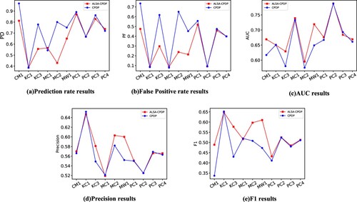
Figure 4. Experimental results of different active learning algorithms.

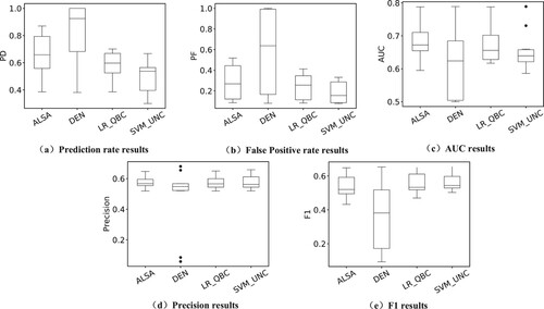
Table 3. Experimental results of different indicators.

	ALSA-CPDP					CPDP
Data	PD	PF	AUC	Precision	F1	PD	PF	AUC	Precision	F1
CM1	0.812	0.475	0.669	0.570	0.489	0.969	0.736	0.617	0.566	0.337
KC1	0.386	0.087	0.650	0.647	0.648	0.386	0.084	0.651	0.652	0.652
KC3	0.556	0.298	0.629	0.581	0.577	0.778	0.618	0.580	0.549	0.430
MC1	0.565	0.086	0.739	0.519	0.516	0.543	0.078	0.733	0.521	0.520
MC2	0.429	0.238	0.595	0.603	0.597	0.800	0.651	0.575	0.582	0.508
MW1	0.650	0.213	0.719	0.600	0.610	0.750	0.452	0.649	0.552	0.473
PC1	0.870	0.519	0.676	0.551	0.432	0.891	0.557	0.667	0.550	0.411
PC2	0.667	0.091	0.788	0.525	0.525	0.667	0.092	0.787	0.525	0.524
PC3	0.828	0.459	0.684	0.566	0.485	0.862	0.475	0.693	0.569	0.480
PC4	0.737	0.399	0.669	0.566	0.513	0.720	0.398	0.661	0.563	0.511
AVG	0.650	0.287	0.682	0.573	0.539	0.737	0.414	0.661	0.563	0.485

Table 4. Experimental results of different active learning algorithms.

Indicator	PD	PF	AUC	Precision	F1
ALSA	0.650	0.287	0.682	0.573	0.539
DEN	0.819	0.590	0.615	0.475	0.357
LR_QBC	0.586	0.242	0.672	0.573	0.557
SVM_UNC	0.496	0.187	0.655	0.576	0.564

Through the analysis of the results, the ALSA method can filter out data with similar defect patterns through the prior knowledge of the target project. Enhanced datasets composed of filtered data and prior knowledge outperform the entire source project data. This shows that the ALSA algorithm retains the samples that contribute more to the defect prediction model and also filters out some noisy data. This verifies the effectiveness of the ALSA algorithm. The algorithm provides a solution for data screening of cross-project software defect prediction.

In our proposed ALSA method, an LR classifier based on an uncertainty sampling strategy is adopted. In the context of cross-project software defect prediction, we denote the density-based sampling strategy as DEN, the algorithm of the committee sampling strategy based on the LR classifier as LR_QBC, and the algorithm of the uncertainty sampling strategy based on the SVM classifier as SVM_UNC. According to the idea of the Burak algorithm, ALSA sets the number of filtered items from the source to be 10 times the number of target items. In comparative experiments, we investigate the performance of LR classifier-based uncertainty sampling strategies with different weights. The source item data is weighted 1–10 times as much as the target item data. Through experiments, the model can obtain the best performance when the amount of filtered source item data is 10 times that of the target item.

Compared with other algorithms, the DEN algorithm has a very high false alarm rate while having a high prediction rate. The performance of the DEN algorithm is unstable, and the performance of Precision and F1 is lower than that of ALSA and CPDP. Analysis of the reasons suggests that a large number of defect-free modules and some noise affect the screening of defective modules. The overall performance of the LR_QBC algorithm and the SVM_UNC algorithm is better than that of DEN. F1 performs better and outperforms the ALSA algorithm, PD and AUC are inferior to the ALSA algorithm. An interpretable reason is that these two algorithms have a deep data mining layer and can show better performance (Liu et al., 2021).

Based on the findings above, we answer RQ1:

1. In summary, the cross-project software defect prediction method based on the ALSA algorithm outperforms the traditional cross-project software defect prediction method.

2. The combination of active learning strategy and classifier is the key to determining the performance of the model, and among various active learning algorithms, the ALSA algorithm shows the best performance.

RQ2: There is still a class imbalance problem with the data filtered from the source project. How effective is it to use active learning methods to solve the problem? What is the optimal sampling rate?

Table 5 and Figure 5 show the effect of different classes of imbalance methods on the results. Among them, ALSA-IM indicates that the imbalance problem is not solved, and ALSA-BL indicates that the imbalance problem is solved using an active learning method. When selecting the data with a high contribution from the source items, it was found that the data still had imbalance problems. The comprehensive performance of the ALSA-BL method was better than random undersampling. The method in this paper is an optimisation of undersampling (Pelayo & Dick, 2007). The problem of randomly deleting data in a random undersampling algorithm is improved by selecting samples according to the ranking of data contributions to modularity.

Figure 5. Performance of imbalance method.

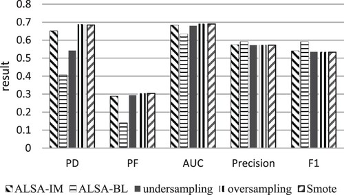
Table 5. Performance of imbalance method.

Indicator	PD	PF	AUC	Precision	F1
ALSA-IM	0.650	0.287	0.682	0.573	0.539
ALSA-BL	0.406	0.139	0.633	0.590	0.579
Undersampling	0.651	0.294	0.678	0.571	0.534
Oversampling	0.688	0.304	0.692	0.573	0.534
Smote	0.684	0.304	0.690	0.572	0.533

By actively selecting data, the best match can be found. The validity of the ALSA method is verified here. When the data is small, the method of over-sampling is usually used. The overall performance of the random oversampling and the smote algorithm is close to that of ALSA. This may be due to the low rate of imbalance in the data being screened (Devi et al., 2019). Compared with the two methods of oversampling, ALSA can obtain the lowest false positive rate while guaranteeing a high prediction rate. It is more widely used in software defect prediction. ALSA can serve as a powerful competitive approach to solving imbalance problems.

From Table 5 and Figure 6, we can understand the performance of the ALSA algorithm and different imbalanced methods. At the same time, the problem of the general equilibrium ratio in the ALSA method is explored. From Table 6, we can see the effect of the balance rate of different weights on the performance. Practice found that when the ratio of defective modules to non-defective modules was 1:3, the overall performance reached its best. When the imbalance rate increased from 1:1 to 1:3, the overall performance showed an upward trend. Overall performance tends to decline at 1:4, so ALSA is at its best at 1:3. One explanation is that the test data in the target project is highly imbalanced, so it is better to have high performance when the source project data meets similar distribution conditions.

Figure 6. Experimental results of different active learning algorithms.

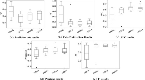
Table 6. Model metrics based on different weights.

Indicator	PD	PF	AUC	Precision	F1
Ratio1	0.539	0.508	0.515	0.506	0.371
Ratio2	0.341	0.211	0.565	0.571	0.520
Ratio3	0.406	0.139	0.633	0.590	0.579
Ratio4	0.425	0.161	0.632	0.581	0.570

Based on the findings above, we answer RQ2:

The ALSA method has the best overall performance and can effectively solve the imbalance problem. The best performance is obtained when the ratio of the number of defective data to the number of non-defective data is 1:3.

RQ3: Compared with traditional WPDP, how does the proposed method perform?

From Table 7 and Figure 7, we can see the performance results of the WPDP algorithm and the balanced cross-project software defect prediction based on the ASLA method. WPDP is the most desirable method for software defect prediction. In this paper, WPDP is used as a baseline to compare with the cross-project software defect prediction method based on the ASLA algorithm to explore the answer to the third question.

Figure 7. WPDP and ALSA algorithm indicator chart.

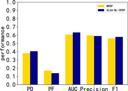
Table 7. Various indicators based on WPDP and ALSA.

	ALSA-BL-CPDP					WPDP
Data	PD	PF	AUC	P	F1	PD	PF	AUC	P	F1
CM1	0.594	0.293	0.650	0.570	0.557	0.333	0.103	0.615	0.609	0.612
KC1	0.183	0.02	0.581	0.725	0.606	0.369	0.094	0.637	0.652	0.644
KC3	0.444	0.191	0.627	0.600	0.608	0.333	0.116	0.609	0.623	0.615
MC1	0.522	0.06	0.731	0.526	0.534	0.265	0.039	0.613	0.522	0.631
MC2	0.457	0.222	0.617	0.627	0.620	0.364	0.099	0.632	0.695	0.636
MW1	0.450	0.101	0.674	0.630	0.647	0.556	0.157	0.699	0.616	0.635
PC1	0.565	0.261	0.652	0.554	0.538	0.328	0.065	0.531	0.626	0.628
PC2	0.333	0.043	0.645	0.525	0.535	0.125	0.038	0.544	0.512	0.515
PC3	0.264	0.097	0.584	0.574	0.578	0.899	0.897	0.501	0.501	0.202
PC4	0.246	0.102	0.572	0.567	0.569	0.242	0.071	0.585	0.614	0.596
AVG	0.406	0.139	0.633	0.590	0.579	0.381	0.168	0.607	0.597	0.561

The results of the two methods can be represented visually in the figure. The software defects based on ALSA are compared with WPDP, and the software defect prediction model constructed by using the ALSA method shows better performance on PD and AUC. In terms of the remaining metrics, WPDP exhibits better experimental results. Through the analysis of the experimental results, the WPDP method uses data from the project, which is a strong guide for the construction of defect models. Although the data filtered through the source project is closer to the data contained in the project, there are still some differences.

Based on the findings above, we answer RQ3:

ALSA and WPDP also show good results. ALSA methods can be augmented with datasets derived from source projects, which can be a powerful competing method in software defect prediction.

6. Threats to validity

This section discusses the external and internal validity of the experiment.

In terms of external validity, there are many data sets in the field of software defect prediction. The public NASA data set used in this paper has been widely used to ensure the representativeness of experiments.

The internal validity reflects the correctness of the experimental results. Common modules in Python are used for data processing in code construction, and the scikit-learn learning package and common hyperparameters are used to build the model. The analysis of the five evaluation indicators allows the accuracy and stability of the model to be considered, and therefore the correctness of the results can be guaranteed. In this paper, the traditional CPDP and the ideal WPDP methods are used as the baseline to make the experiment more convincing. Combining multiple evaluation indexes to analyze the experimental results can ensure the correctness of the results.

In this paper, the use of traditional cross-project software defect prediction methods and intra-project software defect prediction methods are used as baselines that can make the experiments more convincing.

7. Conclusion and future work

In this paper, we propose a cross-project active selection method for software defect prediction, including target and source project selection phases. In the target project selection phase, a combination of clustering algorithms and active learning algorithms is used, and then the data with a high contribution from the target project is filtered for labelling. In the source project selection phase, the annotated data is used as prior knowledge to filter the source projects. Considering the problem of data imbalance, the active learning method is used for balancing. This is a method to optimise the traditional random undersampling method. Finally, a software defect prediction model is constructed using the enhanced dataset.

The proposed method in this paper provides an idea for data filtering in software defect prediction. The method uses active patterns to filter the data and rank the data in terms of contribution, so as to select high-quality data. The augmented dataset is constructed by combining prior knowledge so as to solve the problem of software defect pattern matching. The effectiveness of the proposed method is verified by comparing it with classical software defect prediction methods. However, the proportion of labelled data in the target items is not considered in this paper. The cost of labelling the data is different when constructing a priori knowledge. Also, the impact of feature mapping on the experiments is not considered.

In the future, we hope to conduct in-depth research on the following three aspects: In the first aspect, considering software defect prediction in practical application scenarios, the cost of manual annotation is high. We hope to study the aspects of data acquisition, annotation cost, and algorithm complexity. In the second aspect, we would like to use more active learning methods for research. In the third aspect, we would like to use more models to build the base classifier.

Disclosure statement

No potential conflict of interest was reported by the author(s).

Additional information

Funding

This work is supported by the Xinjiang Tianshan Youth Project of China [grant number: 2020Q019], the National Natural Science Foundation of China [grant number: 61562087], and the Doctoral Scientific Research Foundation of Xinjiang Normal University [grant number: XJNUBS1905].

References

- Bengar, J. Z., van de Weijer, J., Twardowski, B., & Raducanu, B. (2021). Reducing label effort: Self-supervised meets active learning. In 2021 IEEE/CVF International conference on computer vision workshops (ICCVW).https://doi.org/10.1109/iccvw54120.2021.00188
- Bhosle, N., & Kokare, M. (2020). Random forest-based active learning for content-based image retrieval. International Journal of Intelligent Information and Database Systems, 13(1), 72–88. https://doi.org/10.1504/IJIIDS.2020.108223
- Cruz, A. E. C., & Ochimizu, K. (2009). Towards logistic regression models for predicting faultprone code across software projects. 2009 3rd international symposium on empirical software engineering and measurement. https://doi.org/10.1109/esem.2009.5316002
- Devi, D., Biswas, S. K., & Purkayastha, B. (2019). Learning in presence of class imbalance and class overlapping by using one-class SVM and undersampling technique. Connection Science, 31(2), 105–142. https://doi.org/10.1080/09540091.2018.1560394
- Ge, J., Chen, H., Zhang, D., Hou, X., & Yuan, L. (2020). Active learning for imbalanced ordinal regression. IEEE Access, 8, 180608–180617. https://doi.org/10.1109/ACCESS.2020.3027764
- He, P., Li, B., Liu, X., Chen, J., & Ma, Y. (2015). An empirical study on software defect prediction with a simplified metric set. Information and Software Technology, 59, 170–190. https://doi.org/10.1016/j.infsof.2014.11.006
- He, Z., Shu, F., Yang, Y., Li, M., & Wang, Q. (2012). An investigation on the feasibility of cross-project defect prediction. Automated Software Engineering, 19(2), 167–199. https://doi.org/10.1007/s10515-011-0090-3
- Kim, Y. Y., Song, K., Jang, J., & Moon, I. C. (2020). LADA: Look-ahead data acquisition via augmentation for active learning. arXiv preprint arXiv:2011.04194.
- Kitchenham, B. A., Mendes, E., & Travassos, G. H. (2007). Cross versus within-company cost estimation studies: A systematic review. IEEE Transactions on Software Engineering, 33(5), 316–329. https://doi.org/10.1109/TSE.2007.1001
- Li, Y., Huang, Z., Wang, Y., & Fang, B. (2017). Evaluating data filter on cross-project defect prediction: Comparison and improvements. IEEE Access, 5, 25646–25656. https://doi.org/10.1109/ACCESS.2017.2771460
- Li, Y., Wong, W. E., Lee, S. Y., & Wotawa, F. (2019). Using tri-relation networks for effective software fault-proneness prediction. IEEE Access, 7, 63066–63080. https://doi.org/10.1109/ACCESS.2019.2916615
- Liu, W., Hu, E. W., Su, B., & Wang, J. (2021). Using machine learning techniques for DSP software performance prediction at source code level. Connection Science, 33(1), 26–41. https://doi.org/10.1080/09540091.2020.1762542
- Lu, H., Kocaguneli, E., & Cukic, B. (2014). Defect prediction between software versions with active learning and dimensionality reduction. 2014 IEEE 25th international symposium on software reliability engineering. https://doi.org/10.1109/issre.2014.35
- Menzies, T., Butcher, A., Cok, D., Marcus, A., Layman, L., Shull, F., Turhan, B., & Zimmermann, T. (2012). Local versus global lessons for defect prediction and effort estimation. IEEE Transactions on Software Engineering, 39(6), 822–834. https://doi.org/10.1109/TSE.2012.83
- Menzies, T., Milton, Z., Turhan, B., Cukic, B., Jiang, Y., & Bener, A. (2010). Defect prediction from static code features: Current results, limitations, new approaches. Automated Software Engineering, 17(4), 375–407. https://doi.org/10.1007/s10515-010-0069-5
- Nam, J., Pan, S. J., & Kim, S. (2013). Transfer defect learning. 2013 35th international conference on software engineering (ICSE). https://doi.org/10.1109/icse.2013.6606584
- Pelayo, L., & Dick, S. (2007). Applying novel resampling strategies to software defect prediction. NAFIPS 2007 - 2007 annual meeting of the North American fuzzy information processing society. https://doi.org/10.1109/nafips.2007.383813
- Shepperd, M., Song, Q., Sun, Z., & Mair, C. (2013). Data quality: Some comments on the NASA software defect datasets. IEEE Transactions on Software Engineering, 39(9), 1208–1215. https://doi.org/10.1109/TSE.2013.11
- Too, J., & Rahim Abdullah, A. (2020). Binary atom search optimisation approaches for feature selection. Connection Science, 32(4), 406–430. https://doi.org/10.1080/09540091.2020.1741515
- Turhan, B., Menzies, T., Bener, A. B., & Di Stefano, J. (2009). On the relative value of cross-company and within-company data for defect prediction. Empirical Software Engineering, 14(5), 540–578. https://doi.org/10.1007/s10664-008-9103-7
- Turhan, B., Mısırlı, A. T., & Bener, A. (2013). Empirical evaluation of the effects of mixed project data on learning defect predictors. Information and Software Technology, 55(6), 1101–1118. https://doi.org/10.1016/j.infsof.2012.10.003
- Wong, W. E., Debroy, V., Surampudi, A., Kim, H., & Siok, M. F. (2010). Recent catastrophic accidents: Investigating how software was responsible. 2010 fourth international conference on secure software integration and reliability improvement. https://doi.org/10.1109/ssiri.2010.38
- Wong, W. E., Horgan, J. R., Syring, M., Zage, W., & Zage, D. (1998). Applying design metrics to a large-scale software system. Proceedings ninth international symposium on software reliability engineering (Cat. No.98TB100257). https://doi.org/10.1109/issre.1998.730891
- Wong, W. E., Horgan, J. R., Syring, M., Zage, W., & Zage, D. (2000). Applying design metrics to predict fault-proneness: A case study on a large-scale software system. Software: Practice and Experience, 30(14), 1587–1608. https://doi.org/10.1002/1097-024X(20001125)30:14<1587::AID-SPE352>3.0.CO;2-1
- Wong, W. E., Li, X., & Laplante, P. A. (2017). Be more familiar with our enemies and pave the way forward: A review of the roles bugs played in software failures. Journal of Systems and Software, 133, 68–94. https://doi.org/10.1016/j.jss.2017.06.069
- Xu, F., Zhao, H., Zhou, W., & Zhou, Y. (2021). Cost-sensitive regression learning on small dataset through intra-cluster product favoured feature selection. Connection Science, 34(1), 104–123. https://doi.org/10.1080/09540091.2021.1970719
- Xu, Z., Liu, J., Luo, X., & Zhang, T. (2018). Cross-version defect prediction via hybrid active learning with kernel principal component analysis. 2018 IEEE 25th international conference on software analysis, evolution and reengineering (SANER). https://doi.org/10.1109/saner.2018.8330210
- Yuan, Z., Chen, X., Cui, Z., & Mu, Y. (2020). ALTRA: Cross-project software defect prediction via active learning and tradaboost. IEEE Access, 8, 30037–30049. https://doi.org/10.1109/ACCESS.2020.2972644
- Zemmal, N., Azizi, N., Sellami, M., Cheriguene, S., & Ziani, A. (2021). A new hybrid system combining active learning and particle swarm optimisation for medical data classification. International Journal of Bio-Inspired Computation, 18(1), 59–68. https://doi.org/10.1504/IJBIC.2021.117427