Anomaly detection of industrial state quantity time-Series data based on correlation and long short-term memory

ABSTRACT

Anomaly detection of multi-dimensional time-series data is a key research area, and the analysis of control, switching, and other state signals (i.e., industrial state quantity time series) is of particular importance to the operational sciences. When only the limited values of industrial state quantities are taken in the discrete set, there is no continuous change trend, making it difficult to achieve good results when applying analogue anomaly detection methods directly. In this study, assuming a correlation between the time series of state and analogue quantities in industrial systems, a model for anomaly detection in state quantity time-series data is built through a correlation supported by long short-term memory, and the model is verified using real physical process data. These results demonstrate that the proposed method is superior to extant industrial time-series models. Thus far, no studies focusing on the anomaly detection of two-state quantity time-series outliers have been performed. We believe that the research problem addressed herein and the proposed method contribute an interesting design methodology for the anomaly detection of time-series data in IIoT.

KEYWORDS:

• Anomaly detection
• long short-term memory
• machine learning
• model based
• time series of state quantity

1. Introduction

Over the past decade, owing to advancements in informatisation and interconnection, global industries have developed in leaps and bounds. Following the introduction of a variety of intelligent information systems (Wang, 2017a), the intelligent production mode of the industrial internet of things (IIoT), comprising sensors, controllers, intelligent instruments, etc. (Sisinni et al., 2018), has gradually taken shape. In this mode, industrial production activities have served as the carrier and production source of industrial time-series data and have fuelled the application of big data technology (National Manufacturing Strategy Advisory Committee, 2015; Zhang et al., 2016). The analysis and mining of these industrial multi-dimensional time-series data make it possible to control, analyse, decide, and plan the running state of systems, as well as diagnose, alert, dispose, and repair the monitored faults while predicting hidden troubles. In view of the abnormalities in operational data quality defects, equipment failures, performance degradation, and external environmental changes (Lee, 2015; Li, Ni, et al., 2017), a positive cycle of the generation, extraction, and application of effective industrial knowledge (Ding et al., 2020) has come into being via the above processes, particularly in terms of industrial big data (Wang, 2017b). Currently, IIoT time-series data can be classified into two categories: analogue and finite states. Analogue quantities represent the continuous physical changes in a system, such as changes in temperature, pressure, voltage, and current. A time series of finite states refers to equipment that can be in exactly one of a finite number of states at any given time. This paper chiefly analyses the two-state quantity of finite states, such as with a switch.

Presently, numerous detection methods have been proposed for the IIoT anomaly detection of analogue-quantity time series. A survey (Chalapathy & Chawla, 2019) shows the wide application of machine learning in real-world anomaly detection. Moreover, the advantages of long short-term memory (LSTM) units in predicting time series data are leveraged for the IIoT anomaly detection of analogue-quantity time series. Liu, Kumar, et al. (2020) introduced a new on-device federated-learning-based deep anomaly detection framework with a high communication efficiency for sensing time-series data in IIoT based on the convolutional neural network–long short-term memory (AMCNN-LSTM) network. They also introduced an attention mechanism (AM) to improve the performance of this framework (Liu, Garg, et al., 2020).

However, the mentioned methods did not consider the two-state quantity time-series data in IIoT. In some industrial production activities, such as a rocket launch, the requirements for the accuracy of control flow during the launch process are critical. The characteristics of two-state quantity time-series data, which correspond to the control flow, have become increasingly important. Moreover, these time series not only directly reflect the working, fault, and health conditions of equipment, but they also provide essential information for understanding operational conditions and locating system faults. However, two-state quantity time-series data differ from those of analogue quantities, and there is no inherent law of increasing or decreasing trends. The correlation between the series of two-state quantities is subject to the correlation between their corresponding physical quantities. Moreover, because physical processes require a certain response time (e.g. switching a device on or off), there is a time lag between the influence of the state time-series data and the related analogue quantity in the system, making it more difficult (or time consuming) to identify abnormal patterns of two-state quantity time-series data. Through research and analysis, the principal difficulties in research on anomaly detection of industrial time series of two-state quantities are summarised as follows:

• Unlike analogue-quantity time-series data, there is no increase or decrease in the time series of the two-state quantity.

• Unlike analogue-quantity time-series data, the statistical information of the time series of the two-state quantity has a poor effect on the detection of the series.

As shown in Figure 2, when a switch control signal undergoes a change, the change in the corresponding physical quantity is collected by the sensor after a certain delay. Different switches result in different time delays, making it difficult to statistically calculate correlations that accurately reflect the relationship between two-state and analogue-quantity time-series data. In an industrial process, two-state quantity time series do not inherently have obvious change rules, whereas two-state quantity time-series data and their corresponding analogue-quantity time series are heterogeneous. Thus, it is impossible to achieve an ideal detection effect by simply applying the analogue prediction model, which is demonstrated concretely in the experimental section of this paper. By making a general observation of extant methods for time-series anomaly detection, whether based on statistical methods (Enders, 2008) or machine learning (Gao et al., 2002; Qiao et al., 2002; Wang et al., 2006; Zhang et al., 2003), anomaly detection is achieved by analysing and correlating the change rules of the statistical analogue quantity series. Thus, the detection effect of the two-state quantity time series is unsatisfactory. Although machine learning using long short-term memory (LSTM) (Malhotra et al., 2015) has been employed for similar problems, the methods implement anomaly detection using an LSTM unit (Hochreiter & Schmidhuber, 1997) for prediction. Experimental results obtained using such methods reveal poor performance in the anomaly detection of two-state quantity time-series data. From the analysis of a real rocket launch tower, herein, we propose anomaly detection for two-state quantity time-series data based on correlation and LSTM, wherein the correlation is determined using the basic laws of the physical system. Requirements for the control process and LSTM are utilised to learn the rules of interaction between the time series of two-state and correlated analogue quantities. Empirical evaluation shows that the proposed method can efficiently detect anomalies in two-state quantity time series data.

The main contributions of this study can be summarised as follows:

• The proposed method leverages the LSTM and correlation, which are determined by the basic laws of the physical system and requirements for the control process, to achieve the anomaly detection of two-state quantity time-series outliers.

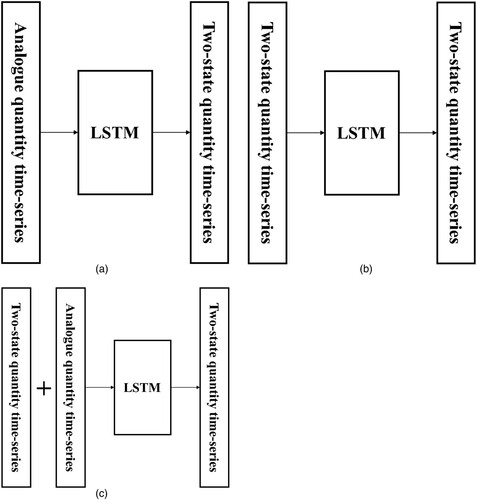
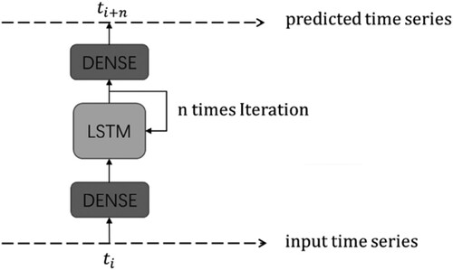
• The proposed method utilises LSTM to learn not only the tendency of time series but also the relationship between the two-state and correlated analogue quantity time series, as shown in Figure 1(c). Figure 1(b) and (c) show two direct applications of LSTM.

• The proposed method is compared with AR, naive, and direct application of LSTM, to show its efficiency.

Figure 1. The differences between the LSTM unit application, the proposed method, and the traditional ways. (a) Utilized LSTM to learn the relationship between the two-state quantity time series and correlated analogue quantity time series. (b) Direct applications of LSTM with only the two-state quantity time series. (c) Direct applications of LSTM with the two-state quantity time series and correlated analogue quantity time series.

Thus far, no studies focusing on the anomaly detection of two-state quantity time-series outliers have been performed. We believe that the research problem addressed herein and the proposed method contribute an interesting design methodology for the anomaly detection of time-series data in IIoT.

The remainder of this paper is organised as follows. Section 2 discusses relevant theories and definitions, concrete models, and related algorithms that support the study. Section 3 elaborates on the setup, analysis, and results of the experiments, and Section 4 summarises the findings and postulates the scope for future research.

2. Related works

In the literature, there are three primary methods for detecting time-series data anomalies (Mehrotra et al., 2017). One is the similarity-measurement-based method, which involves data representation and similarity calculation to find corresponding anomalies (Park & Kim, 2017). The second involves time-series data clustering and assigning an anomaly score to each data pattern. The third method is model based (Li, Pedrycz, et al., 2017; Ren et al., 2017).

2.1. Similarity-measurement-based method

The similarity-measurement-based method consists of two stages: data representation and similarity measurement. There are many data representation methods, such as piecewise linear representation, which involves selecting some important data points from the original data, connecting these points head-to-tail with line segments, and using line segments to fit the data (Shang & Sun, 2010). This method has good performance and data volume reduction, but it ignores detailed information. The piecewise aggregate approximation method divides time-series data into sub-sequences of equal length and represents each by its mean, which may result in information loss of the data-changing tendency (Nakamura et al., 2013). The symbolic aggregate approximation method represents time-series data as characters. It divides the range space distribution of the data into several subrange spaces of equal probability (Kolozali et al., 2016). Different subrange spaces are represented by different characteristics. The disadvantage of this method is that the character operation rules must be defined. Discrete Fourier transform and discrete wavelet transform methods transform time-series data from the time domain to the frequency domain and represent the data as features of the frequency domain (Chaovalit et al., 2011; Dwivedi & Subba Rao, 2011). The singular value decomposition method represents time-series data using matrix transformations (Varasteh Yazdi & Douzal-Chouakria, 2018).

2.2. Clustering-based method

The clustering-based method involves clustering time-series data and assigning an anomaly score to each pattern according to the revealed cluster centres. The classic fuzzy C-means clustering method clusters and reconstructs time-series data according to the revealed clustering centres. Reconstruction errors between the original time-series data and the reconstructed data are utilised to assign corresponding anomaly scores to each pattern in the time series (Izakian et al., 2015). The corresponding cluster centroids obtained by the K-means clustering method are utilised as patterns for computationally efficient distance-based detection of anomalies in new monitoring data (Münz et al., 2007). Rank-based algorithms provide a promising approach for anomaly detection (Huang et al., 2012) because the concept of modified rank is introduced, and a clustering algorithm for anomaly detection is provided.

2.3. Model-based method

There are various models for anomaly detection, such as auto regression (AR) and moving average (MA); the ARMA model is a mixture of these two. Using ARMA, it is assumed that there are no anomalies in the training data and that a model is trained to establish a model and threshold value. The prediction values for each set of test data are made available from the model, and anomalies are determined according to the threshold value (Van Der Voort et al., 1996). LSTM is a classical neural network model used for anomaly detection. Like ARMA, LSTM (Karim et al., 2018) requires training data and is more widely used than ARMA. A Markov model trains a classical model with training data so that one can obtain the initial probability, the state transition matrix, and its threshold value (Ren et al., 2017). Because the Markov model analyses each datum in the process of anomaly detection, it is suitable for detecting point anomalies and has high detection accuracy. However, owing to the nature of time-series data, an anomaly often does not appear in the form of a single point (Li, Pedrycz, et al., 2017 ). When an anomaly occurs at a data point, the data before and after this anomaly are abnormal, providing a pattern anomaly. Moreover, Liu, Kumar, et al. (2020) introduced a new communication-efficient on-device federated learning deep anomaly detection framework for sensing time-series data in IIoT via the Convolutional Neural Network-Long Short-Term Memory (AMCNN-LSTM). They also introduced Attention Mechanism (AM) to improve the performance of this framework (Liu, Garg, et al., 2020). Unfortunately, these methods mentioned above are not designed for state-quantity time series. To address this problem, we propose a new LSTM model with correlation.

3. Proposed method

3.1. Anomaly detection of two-state time series

There exist correlations between two-state (e.g. control and echo signals) and analogue-quantity time series (e.g. physical signals). Two-state quantity time-series anomaly detection can be achieved by studying the laws of these correlations. However, there is a time lag between the two-state and analogue-quantity time series, as displayed in Figure 2.

Figure 2. Time lag in the correlation between the time series of two-state quantity composed of a two-state control signal and an analogue quantity reflecting the physical quantity change corresponding to two-state control signals. (a) Switching process for switching in a space tower. (b) Switching on the process. (c) Switching off the process.

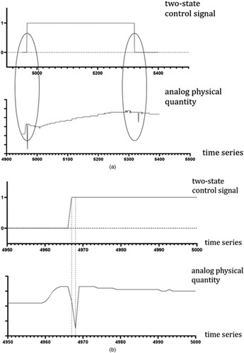
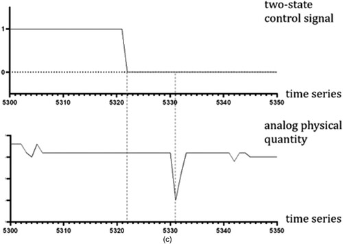
Figure 2(a) shows the process of opening and closing a switch in the space launch tower. When the switch is turned on, it inevitably causes the corresponding pipeline pressure to change. As shown in Figure 2(b) and (c), there are temporal delays with the changes of the control signal from zero to one and vice versa.

These observations suggest that a study of this correlation will reflect a time series rather than a one-to-one mapping. Based on this, LSTM, which has advantages in predicting time series data, is utilised to learn this correlation so that the outlier of the time series of the two-state quantity can be detected.

3.2. Basic definition

Definition 1 (set of time points): T is a set of time points, denoted as $T=\{t_i{\}}_{i=1}^N$, where N is the number of time points.

Definition 2 (time series of two-state quantity): The time series of the two-state quantity is a series of control signals and return signals of zero and one. The two-state quantities are sampled and captured by sensors. A time series of two-state quantities with a length of N is expressed as S = ($s_1$,$s_2$,$s_1$, … , $s_N$), in which each element is a binary group, $s_i$ = ($x_i$, $t_i$), $x_i$ is zero or one, and $t_i$ is the time recording point. For any integers, i and j, if i < j, the $\text{n }{t}_i$<$t_j$.

Definition 3 (time-series group of two-state quantity): S is a time-series set of two-state quantities containing K sets with the same time point, T, denoted as S = {${\mathit{S}}_1$, ${\mathit{S}}_2$, ${\mathit{S}}_3$, … , ${\mathit{S}}_{\mathit{k}}$,}. S is the time-series group of the two-state quantity of the K^th dimension.

Definition 4 (time series of analogue quantity): The time series of analogue quantity is a series of continuous data points sampled and captured by sensors. A time series of analogue quantity with length N is expressed as S = ($s_1$, $s_2$, $s_1$, … , $s_N$), where each element is a binary group, $s_i$ = ($x_i$, $t_i$), $x_i$ is a real value, and $t_i$ is the time recording point. For any integers, i and j, if i < j, then $t_i$<$t_j$.

Definition 5 (time-series group of analogue quantity): S is a time-series set of two-state quantities containing K sets with the same time point, T, which is denoted as S = {${\mathit{S}}_1$, ${\mathit{S}}_2$, ${\mathit{S}}_3$, … , ${\mathit{S}}_{\mathit{k}}$,}. S is the time-series group of the two-state quantity of the Kth dimension.

Definition 6 (time-series segment): The time interval of the set, T[i:j] (i < j<N), refers to the collection of all time points from $t_i$ to $t_j$ (including and $t_i$ and $t_j$) intercepted from the set of time points, T, where T[i:j]∈T.

Definition 7 (normal and abnormal modes of the time series of two-state quantity): S is the time-series group of two-state quantity of K dimensions on the set of time points, T, and the zero and one arrangement of K-dimensional vector elements of S at time point t is the mode of S at time point t, where t ∈ T. The mode that exists in S without errors is the normal mode, whereas the mode that does not exist is the abnormal mode.

Definition 8 (outlier of the time-series group of two-state quantity): The anomaly of the time-series group of two-state quantity chiefly covers two situations:

• When the time-series group of the two-state quantity appears in the anomaly model on ${\text{T}}_1$ at the set of time points, it is said that the time series of the two-state quantity has an outlier at ${\text{T}}_1$.

• Assuming the time-series group of the two-state quantity on ${\text{T}}_1$ at the set of time points should be Model 1, but the actual time-series group of two-state quantity is Model 2 on this time-series segment, it is said that the time series of two-state quantity has an outlier on ${\text{T}}_1$.

3.3. Method of anomaly detection

In this study, the machine learning model is trained to learn the correlation function, F(S) = s, between analogue and two-state quantity time series, where S represents the analogue-quantity time-series group in a certain segment, and s represents the two-state quantity time-series group at a time point. Using the learned correlation function, F, the two-state quantity time-series group can be predicted from the analogue-quantity time-series group after undergoing anomaly detection. Finally, it can be determined whether the actual value belongs to the outlier of the two-state time-series group by comparing the differences between the predicted and actual values. Because the outlier of the two-state quantity time-series group is detected using the correlation between the two-state and analogue-quantity time-series groups, it includes the two outliers of the two-state quantity time-series group, as per Definition 8.

3.4. Introduction to the model

3.4.1. Introduction to LSTM

An LSTM is a special kind of recurrent neural network that can be used to learn long-term dependencies. LSTM performs well and is extensively used with natural language models in which historical information must be considered. An LSTM network is recursive, with a chain repeating neural networks. Because there may be a lag of unknown duration between important events in a time series, the LSTM network is highly suitable for classification, processing, and prediction. Wu et al. (2022) and Gao et al. (2021) utilised LSTM to achieve prediction in stock and missing data respectively. Zhang et al. (2021) utilised LSTM to achieve detection in mental fatigue. Further, by controlling the number of recursions, an LSTM can adapt to unlimited scenarios with different timing rules. Experiments on the dataset of a real rocket launch suggest that the LSTM network can be used to efficiently learn the complex correlations between analogue and two-state time series in this dataset.

3.4.2. Introduction to the machine learning model structure

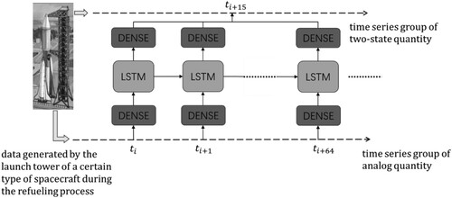
The machine learning model proposed in this study comprises two fully connected layers and a common LSTM unit. The analogue-quantity time-series group in the training dataset is normalised as input to the LSTM unit after weight allocation through a fully connected layer. After iterative calculations, x is output and integrated into the predicted value, s, through the last fully connected layer. The model is trained by calculating the mean square error (MSE) of the predicted value, s, and the actual value of the corresponding two-state quantity time-series group in the training dataset as the loss value. Meanwhile, the activation functions of the two fully connected layers in the model use the Relu () function because the value of the analogue-quantity time series generally takes a linear change, and the occurrence probability of a zero or one state in the industrial two-state quantity time-series group has no clear rule. In view of the characteristics of actual industrial datasets, to learn the correlation rule between the analogue and two-state quantity series, this study uses the analogue-quantity time-series group at T[$t_i$: $t_{i+64}$] as training input. This takes the two-state quantity time-series group at $t_{i+15}$ as the corresponding actual value for one operation and extracts the relationship between the analogue-quantity time-series group of the set of time points from $t_i$ to $t_{i+64}$ and the two-state quantity time-series group at $t_{i+15}$, in which the selected set of time points from $t_i$ to $t_{i+64}$ and time point $t_{i+15}$ is designed by observing the actual data, as displayed in Figure 3. The model training and detection algorithm of the outlier is demonstrated in detail in Algorithm 1.

Figure 3. The framework of the proposed anomaly detection. LSTM, long short-term memory. (a) Precision (P). (b) Recall (R).

Table

Algorithm 1. Model training.

Input: ${\mathit{S}}_1$, ${\mathit{S}}_2$

1: ${\mathit{S}}_1$, ${\mathit{S}}_2$ = Train_dataset

# where ${\mathit{S}}_1$ is time-series group of two-state quantity, ${\mathit{S}}_2$ is time-series group of analogue quantity

2: N = length(${\mathit{S}}_1$)

3. Mem = Init()

# Use public LSTM model to initialise Mem

4. For i in range(0,N-64):

5.  For j in range(0,64):

6.   Input + =  ${\mathit{S}}_1$ [i + j]

7.   Y, Mem = Model(Input)

8. Loss = mse(Y, ${\mathit{S}}_2$ [i+15])

9. Backward()

Output: Model

3.4.3. Introduction to anomaly detection algorithm

In this study, the prediction function, F(), based on the correlation between the two-state quantity time-series group and its corresponding analogue-quantity time-series group is acquired by training the model from Section 3.4.2. The anomaly detection algorithm is shown in Algorithm 2. First, the analogue-quantity time-series group in the set of time points, T, to be detected is grouped per the time period of T[$t_i$: $t_{i+64}$] (i∈[0,N],T∈T) as the input of function F () to obtain the corresponding predicted value, x. By calculating the MSE between the predicted value, x, and the value, s, to be detected in the corresponding two-state quantity time series, it is judged whether the detected value, s, is abnormal.

The analysis of the time and space complexity of Algorithm 2, which is utilised to achieve the anomaly detection of two-state quantity time-series outliers, is as follows. Algorithm 2 includes two parts: (i) the prediction part and (ii) the anomaly judgement part. Both these parts have the same time complexity, i.e. O(n). Thus, the time complexity of Algorithm 2 is O(n). The space complexity of these two parts is O(1).

Table

Algorithm 2. Outlier calculation method.

Input: ${\mathit{S}}_1$, ${\mathit{S}}_2$

1: ${\mathit{S}}_1$, ${\mathit{S}}_2$ = Train_dataset

# where S_1 is time-series group of two-state quantity, ${\mathit{S}}_2$ is time-series group of analogue quantity

2. N = length(${\mathit{S}}_1$)

3. Anomaly =

# Anomaly is used to record time points of outlier

4. For i in range(0,N-64):

5.  For j in range(0,64):

6.   Input = ${\mathit{S}}_1$ [i + j]

7.  Y = Model(Input)

# Model is the well-trained anomaly detection model

8.  Loss = mse(Y, ${\mathit{S}}_2$ [i + 15])

9.  If (Loss > 0.1):

10.   Anomaly.append(i + 15)

11. Return Anomaly Output: Anomaly

4. Experimental verification

4.1. Experimental definition

4.1.1. Dataset

In this study, the tower data of a new type of domestic rocket prior to launch were used for the experiment. We used the data of the first two of the last three tasks as the training set. The data included the 29-dimensional analogue-quantity time-series group and the 12-dimensional two-state quantity time-series group. There were 42,262 time points collected for each task, and 126,786 time points were collected for the three tasks.

4.1.2. Algorithms for comparison

In the experiment, we performed all algorithms mentioned above as a correlation and LSTM-based anomaly detection (CLAD) process. To objectively verify the performance of this method, we implemented three time-series anomaly detection methods as benchmark algorithms and performed performance comparison experiments. The AR algorithm (Enders, 2008) is a basic algorithm of series anomaly detection based on statistics, which maintains a dynamic window with a length, k, and it calculates the mean, variance, and other statistical characteristic values of the series in the window to predict whether the actual data value of the (k+1) window conforms to the prediction of the algorithm. If not, it is deemed an anomaly. The traditional LSTM anomaly detection (LSTM-AD) algorithm (Malhotra et al., 2015) predicts the time series using the LSTM unit and determines the outlier by calculating the distance between the predicted and actual value, as shown in Figures 1(b), 1(c) and 4. The naive model, which utilises previous data to predict the subsequent data, is the simplest prediction model, but it is efficient. In the experiment, the LSTM unit from the keras package is leveraged to develop the mentioned LSTM-related methods. There is one hyperparameter: N, the number of nodes in the hidden layer and its default value is 70 at which CLAD performs best.

Figure 4. Long short-term memory (LSTM) anomaly detection algorithm model. (a) Correct time series of two-state quantity. (b) Predicted time series generated via CLAD. (c) Predicted time series generated via LSTM-AD-S.

4.1.3. Calculation index

There are two categories of objectives classified in this study; positive and negative instances include normal and abnormal data, respectively. Taking the time-series group as an instance unit, the experimental results can be classified into the following four categories:

1. True positives (TP): the number of instances that are normal and detected as normal by the algorithm.

2. False positives (FP): the number of instances that are abnormal but detected as normal by the algorithm.

3. False Negatives (FN): the number of instances that are normal but detected as abnormal by the algorithm.

4. True Negatives (TN): the number of instances that are abnormal and detected as abnormal by the algorithm.

5. Precision (P): $P=\frac{TP}{TP+FP}$

6. Recall (R): $R=\frac{TP}{TP+FN}$

7. f1 score: $f1=2\ast \frac{P\ast R}{P+R}$

8. True Positive Rate (TPR): $TPR=\frac{TP}{TP+FN}$

9. False Positive Rate (FPR): $FPR=\frac{FP}{FP+TN}$

After classifying the results, we can evaluate the performance of the algorithm by calculating the accuracy and recall rates. At 42,262 time points in the test set, the researcher randomly set abnormal instances in the 12-dimensional two-state quantity time series and made five test groups. The numbers of abnormal instances in the test groups were 12,000, 14,000, 16,000, 18,000, and 20,000, respectively.

4.2. Effectiveness of the algorithm

This study tested the influence of the total number of abnormal instances on the three given methods. In the experiment, the AR algorithm was used to directly act on the test group. Two groups of experiments were conducted to guarantee fairness in the amounts of information when using LSTM-AD. In the first group, only the two-state quantity time-series group was used as the input series (hereinafter referred to as LSTM-AD-S). In the second group, both two-state and analogue-quantity time-series groups were used as input (hereinafter referred to as LSTM-AD-D).

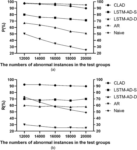
The experimental results are shown in Figure 5. Primarily, with the increase in the total number of abnormal data, both P and R values of the AR algorithm are low, indicating the worst performance. Conversely, with the increase in the total number of abnormal data, both P and R values exhibited a clear decrease, suggesting that the AR algorithm cannot be used to extract the characteristics of the zero-to-one two-state quantity time series. Further, the P value of the CLAD algorithm is close to that of the naive model; specifically, the P value difference is 1.1% on average, and the R value of CLAD is 31.5% higher than that of the naive model on average. Compared with the traditional LSTM-AD-S algorithm, the CLAD algorithm proposed in this study resulted in higher P and R values. With the increasing number of abnormal instances, the accuracy of both the LSTM-AD-S and CLAD algorithms decreased, but the P value of the CLAD algorithm remained above 89.8%, and the R value was stable between 89.7% and 92.3%. This indicates that the detection strategy based on correlation between the corresponding two-state and analogue-quantity time-series groups designed in this study maintained a stable detection effect with excellent performance under complex data conditions of numerous anomalies. Finally, comparing the experimental results of LSTM-AD-S and LSTM-AD-D, it can be observed that in the case of LSTM-AD-D, two-state and analogue-quantity time-series groups were input into the LSTM-AD model simultaneously, in contrast to only using the two-state quantity time-series group as the input; thus, this model was provided with a larger amount of information. However, as the data structures of the two-state and analogue-quantity time-series groups were heterogeneous, the outlier detection performance of LSTM-AD-D was inferior to that of LSTM-AD-S, which only received the two-state quantity time-series group as the input. Specifically, in the five experimental groups, the P value of LSTM-AD-D was 13.3% lower than that of LSTM-AD-S, and the R value was 10.1% lower than the average. This reveals that the LSTM prediction network was not effective for direct outlier detection in heterogeneous data.

Figure 5. Experimental results.

In Figure 6, the receiver operating characteristic (ROC) of CLAD, LSTM-AD-S, LSTM-AD-D, and AR is shown, and the area under the curve (AUC) is presented in Table 1, in which the average P, average R, and f1 score are listed. In conclusion, the proposed CLAD is efficient in the anomaly detection of industrial two-state quantity time-series data. In Table 2, the performance of CLAD with different N is shown. The results show that CLAD is not sensitive to the hyperparameter, N, in the range from 50 to 110 with the best performance at 70 and decreases obviously when N is less than 30. Moreover, from Figure 7, it is observed that the predicted time series generated by CLAD are more similar to the correct time series of the two-state quantity than those generated by LSTM-AD-S.

Figure 6. ROC results.

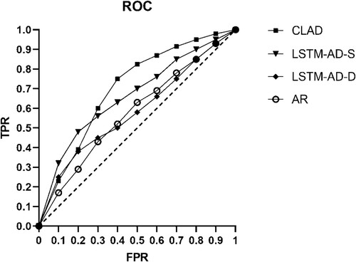
Figure 7. Time series of two-state quantity generated via LSTM-AD-S, LSTM-AD-D, and CLAD on three certain time-series segments.

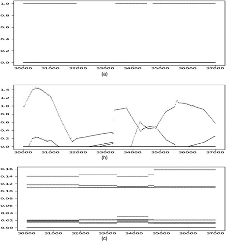
Table 1. Average precision, average recall, f1 score, and AUC of CLAD, LSTM-AD-S, LSTM-AD-D, AR, and naive.

Method	Average precision (%)	Average recall (%)	f1 score	AUC
CLAD	94.4	91.1	0.927	0.742
LSTM-AD-S	75.1	68.9	0.719	0.705
LSTM-AD-D	59.3	58.5	0.589	0.627
AR	36.4	26.7	0.308	0.619
Naive	96.5	59.6	0.737	–

Table 2. Average precision, average recall, and f1 score of CLAD with different hyperparameter, N.

N	Average precision (%)	Average recall (%)	f1 score
10	72.4	70.1	0.712
30	87.2	84.5	0.858
50	94.2	90.7	0.924
70	94.4	91.1	0.927
90	93.8	90.1	0.919
110	90.4	89.2	0.898

5. Conclusion

This paper solved the anomaly detection problem of zero-to-one time-series data based on correlation and LSTM machine modelling and respectively introduced a new model structure and anomaly detection algorithm. With several experiments on datasets from a real manufacturing industry, this study verified that the proposed method can be used to address the problem of anomaly detection of industrial two-state quantity time-series data in a limited way, and its accuracy and efficiency are significantly better than existing methods based on statistics and LSTM. Future research directions include improving the network structure and developing unsupervised or weakly supervised models, as well as boosting the learning performance of the model by enhancing the public LSTM unit or combining other functional units, such as variational autoencoders and generative adversarial networks.

Disclosure statement

No potential conflict of interest was reported by the author(s).

Additional information

Funding

This work was supported by the Independent and open subject fund [grant number 202101-10] from State Key Laboratory of High-Performance Computing and the National Key Research and Development Program of China [grant number 2018YFB0204301].

Notes on contributors

Mingxin Tang

Mingxin Tang, B.Sc., is currently a master's student at the College of Computer, National University of Defence Technology. His main research interests include artificial intelligence. E-mail: [email protected]

Wei Chen

Wei Chen, Ph.D., is a Professor of the College of Computer, National University of Defence Technology. Her main research interests include computer system structure and artificial intelligence. E-mail: [email protected]

Wen Yang

Wen Yang, Ph.D., is currently a senior engineer at the Key Laboratory of Space Launching Site Reliability Technology. His research interests include industrial big data, industrial intelligence, and prognostics health management. E-mail: [email protected]

References

- Chalapathy, R., & Chawla, S. (2019). Deep learning for anomaly detection: A survey. arXiv preprint arXiv:1901.03407.
- Chaovalit, P., Gangopadhyay, A., Karabatis, G., & Chen, Z. (2011). Discrete wavelet transform-based time series analysis and mining. ACM Computing Surveys, 43(2), 1–37. https://doi.org/10.1145/1883612.1883613
- Ding, X. O., Yu, S. J., Wang, M. X., Wang, H. Z., Gao, H., & Yang, D. H. (2020). Anomaly detection on industrial time series based on correlation analysis. Ruan Jian Xue Bao/Journal of Software, 31(3), 726–747 (in Chinese). https://doi.org/10.13328/j.cnki.jos.005907
- Dwivedi, Y., & Subba Rao, S. (2011). A test for second-order stationarity of a time series based on the discrete Fourier transform. Journal of Time Series Analysis, 32(1), 68–91. https://doi.org/10.1111/j.1467-9892.2010.00685.x
- Enders, W. (2008). Applied econometric time series. John Wiley & Sons.
- Gao, B., Ma, H. Y., & Yang, Y. H. (2002). Hmms (hidden Markov models) based on anomaly intrusion detection method. In Bo Gao, Hui-Ye Ma, & Yu-Hang Yang (Eds.), Proceedings of the international conference on machine learning and cybernetics, 1 (pp. 381–385).
- Gao, K., Chang, C.-C., & Liu, Y. (2021). Predicting missing data for data integrity based on the linear regression model. International Journal of Embedded Systems, 14(4), 355–362. https://doi.org/10.1504/IJES.2021.117946
- Hochreiter, S., & Schmidhuber, J. (1997). Long short-term memory. Neural Computation, 9(8), 1735–1780. https://doi.org/10.1162/neco.1997.9.8.1735
- Huang, H., Mehrotra, K., & Mohan, C. K. (2012). Algorithms for detecting outliers via clustering and ranks. Lecture Notes in Computer science, Proceedings of the International Conference on industrial, engineering, and other Applications of Applied intelligent systems (pp. 20–29). Berlin, Heidelberg: Springer. https://doi.org/10.1007/978-3-642-31087-4_3.
- Izakian, H., Pedrycz, W., & Jamal, I. (2015). Fuzzy clustering of time series data using dynamic time warping distance. Engineering Applications of Artificial Intelligence, 39, 235–244. https://doi.org/10.1016/j.engappai.2014.12.015
- Karim, F., Majumdar, S., Darabi, H., & Chen, S. (2018). LSTM fully convolutional networks for time series classification. IEEE Access, 6(99), 1662–1669. https://doi.org/10.1109/ACCESS.2017.2779939
- Kolozali, S., Puschmann, D., Bermudez-Edo, M., & Barnaghi, P. (2016). On the effect of adaptive and nonadaptive analysis of time-series sensory data. IEEE Internet of Things Journal, 3(6), 1084–1098. https://doi.org/10.1109/JIOT.2016.2553080
- Lee, J. (2015). Industrial big data: The revolutionary transformation and value creation in INDUSTRY 4.0 era (B. H. Qiu, Trans.). China Machine Press. (in Chinese).
- Li, J., Ni, J., & Wang, A. Z. (2017). From big data to intelligent manufacturing. Shanghai Jiao Tong University Press. (in Chinese).
- Li, J., Pedrycz, W., & Jamal, I. (2017). Multivariate time series anomaly detection: A framework of hidden Markov models. Applied Soft Computing, 60, 229–240. https://doi.org/10.1016/j.asoc.2017.06.035
- Liu, Y., Garg, S., Nie, J., Zhang, Y., Xiong, Z., Kang, J., & Hossain, M. S. (2020). Deep anomaly detection for time-series data in industrial IoT: A communication-efficient on-device federated learning approach. IEEE Internet of Things Journal, 8(8), 6348–6358. https://doi.org/10.1109/JIOT.2020.3011726
- Liu, Y., Kumar, N., Xiong, Z., Bryan Lim, W. Y., Kang, J., & Niyato, D. (2020). Communication-efficient federated learning for anomaly detection in industrial internet of things. Globecom 2020–2020 IEEE Global Communications Conference, Taipei, Taiwan.
- Malhotra, P., Vig, L., Shroff, G., & Agarwal, P. (2015). Long short-term memory networks for anomaly detection in time series. Proceedings of the European symposium on artificial neural networks, Computational intelligence, and machine learning (pp. 89–94).
- Mehrotra, K. G., Mohan, C. K., & Huang, H. (2017). Anomaly detection principles and algorithms. Springer International Publishing.
- Münz, G., Li, S., & Carle, G. (2007). Traffic anomaly detection using k-means clustering. Proceedings of the GI/ITG workshop MMBnet (pp. 13–14).
- Nakamura, T., Taki, K., Nomiya, H., Seki, K., & Uehara, K. (2013). A shape-based similarity measure for time series data with ensemble learning. Pattern Analysis and Applications, 16(4), 535–548. https://doi.org/10.1007/s10044-011-0262-6
- National Manufacturing Strategy Advisory Committee. (2015). Made in China 2025. Technology road map for key areas (in Chinese).
- Park, J. W., & Kim, D. Y. (2017). Standard time estimation of manual tasks via similarity measure of unequal scale time series. IEEE Transactions on Human-Machine Systems, 48(3), 241–251. https://doi.org/10.1109/THMS.2017.2759809
- Qiao, Y., Xin, X. W., Bin, Y., & Ge, S. (2002). Anomaly intrusion detection method based on HMM. Electronics Letters, 38(13), 663–664. https://doi.org/10.1049/el:20020467
- Ren, H., Ye, Z., & Li, Z. (2017). Anomaly detection based on a dynamic Markov model. Information Sciences, 411, 52–65. https://doi.org/10.1016/j.ins.2017.05.021
- Shang, F. H., & Sun, D. C. (2010). PLR based on time series tendency turning point. Application Research of Computers, 6, 27.
- Sisinni, E., Saifullah, A., Han, S., Jennehag, U., & Gidlund, M. (2018). Industrial internet of things: Challenges, opportunities, and directions. IEEE Transactions on Industrial Informatics, 14(11), 4724–4734. https://doi.org/10.1109/TII.2018.2852491
- Van Der Voort, M., Dougherty, M., & Watson, S. (1996). Combining Kohonen maps with Arima time series models to forecast traffic flow. Transportation Research Part C: Emerging Technologies, 4(5), 307–318. https://doi.org/10.1016/S0968-090X(97)82903-8
- Varasteh Yazdi, S. V., & Douzal-Chouakria, A. (2018). Time warp invariant kSVD: Sparse coding and dictionary learning for time series under time warp. Pattern Recognition Letters, 112, 1–8. https://doi.org/10.1016/j.patrec.2018.05.017.
- Wang, J. M. (2017a). White paper on big data technology and application in China’s industry. Alliance of Industrial Internet (in Chinese).
- Wang, J. M. (2017b). Summary of industrial big data technology. Big Data Research, 6, 3–14. https://doi.org/10.11959/j.issn.2096-0271.2017057. (in Chinese with English abstract ).
- Wang, M., Zhang, C., & Yu, J. (2006). Native API based windows anomaly intrusion detection method using SVM. Proceedings of the IEEE International Conference on Sensor Networks 1:6.
- Wu, S., Liu, Y., Zou, Z., & Weng, T. (2022). S_I_LSTM: Stock price prediction based on multiple data sources and sentiment analysis. Connection Science, 34(1), 44–62. https://doi.org/10.1080/09540091.2021.1940101
- Zhang, J., Qin, W., Bao, J. S., et al. (2016). Big data in manufacturing industry. Shanghai Science and Technology Press (in Chinese).
- Zhang, S., Zhang, Z., Chen, Z., Lin, S., & Xie, Z. (2021). A novel method of mental fatigue detection based on CNN and LSTM. International Journal of Computational Science and Engineering, 24(3), 290–300. https://doi.org/10.1504/IJCSE.2021.115656
- Zhang, X., Fan, P., & Zhu, Z. (2003). A new anomaly detection method based on hierarchical HMM. Proceedings of the 4th International Conference on Parallel and Distributed Computing, Applications, and Technologies (pp. 249–252).