Multi-Semantic Alignment Graph Convolutional Network

ABSTRACT

Graph Convolutional Network (GCN) is a powerful emerging deep learning technique for learning graph data. However, there are still some challenges for GCN. For example, the model is shallow; the performance is poor when labelled nodes are severely scarce. In this paper, we propose a Multi-Semantic Aligned Graph Convolutional Network (MSAGCN), which contains two fundamental operations: multi-angle aggregation and semantic alignment, to resolve two challenges simultaneously. The core of MSAGCN is the aggregation of nodes that belong to the same class from three perspectives: nodes, features, and graph structure, and expects the obtained node features to be mapped nearby. Specifically, multi-angle aggregation is applied to extract features from three angles of the labelled nodes, and semantic alignment is utilised to align the semantics in the extracted features to enhance the similar content from different angles. In this way, the problem of over-smoothing and over-fitting for GCN can be alleviated. We perform the node clustering task on three citation datasets, and the experimental results demonstrate that our method outperforms the state-of-the-art (SOTA) baselines.

KEYWORDS:

• Graph convolutional network
• multi-semantic alignment
• semantic alignment
• GCN

View correction statement:

Correction

1. Introduction

GCN is a powerful graph data tool that can naturally integrate node information and topology. It has many suitable application scenarios, such as social networks (Bian et al., 2020; J. Hu et al., 2021), knowledge tracing (Song et al., 2022, 2021; Y. Yang et al., 2021), traffic prediction (N. Hu et al., 2021; Zhao et al., 2022), and environmental monitoring (Chang et al., 2021). In addition, GCN is also widely used in computer vision (Tan et al., 2020), recommender systems (Wang et al., 2019), and natural language processing (Mishra et al., 2019).

The basic process of GCN is to aggregate node information iteratively from local graph neighbourhoods and propagate it through the graph after feature transformation. It is usually grouped into two methods: spatial convolution and spectral convolution. The spatial convolution method defines the convolution operation on the spatial relations of the nodes, learning and updating the representation from their neighbourhoods. For example, Hamilton et al. (2017) proposed a generic induction framework, GraphSAGE, which exploits node feature information to generate node embeddings for unknown data. Atwood and Towsley (2016) designed diffusion convolutional neural networks (DCNN) that learn diffusion-based representations from graph-structured data and utilise them for node classification. Monti et al. (2017) suggested a unified framework called MoNet that generalises convolutional neural network architectures to non-Euclidean domains. In addition, Veličković et al. (2017) included a graph attention network (GAT) that assigns personalised weights to neighbouring nodes by stacking layers in which nodes can participate in their neighbourhood features.

On the other hand, the spectral convolution method implements the convolution operation on the topological map using spectral map theory. For example, Bruna et al. (2013) first proposed a CNN network that extended to graphs based on spectral graph theory. Then, Defferrard et al. (2016) suggested the ChebNet model, which reduces the computational complexity by defining the filter as a Chebyshev polynomial of the diagonal matrix of the eigenvectors. Based on the previous work, Kipf and Welling (2016) introduced a simple and effective layer propagation method with a first-order approximation to simplify the calculation method. In addition, Wu et al. (2019) designed a simple graph convolution (SGC) that captures higher-order information in a graph by a single linear function.

Despite its remarkable success, GCN has two significant limitations. The first limitation is that GCN performance weakens when there are few labelled nodes in each class, and it can easily lead to an over-fitting phenomenon. GCN propagates features through the graph structure, and labels cannot propagate the whole graph when the nodes are sparse. The second limitation is that most of the existing GCN is usually shallow, and Kipf and Welling (2016) showed that the most optimal performance was obtained with a 2-layer model. Q. Li et al. (2018) explained that the essence of GCN is to make a linear combination of each node's neighbouring features and its features. When there are too many stacking layers, the features of nodes aggregate too many neighbouring features, which can lead to the over-smoothing problem, i.e. the nodes become similar to each other and similar between classes. M. Liu et al. (2020) demonstrated that GCN could lead to the over-fitting phenomenon for indistinguishable features of nodes while expanding the perceptual field by stacking multiple hidden layers.

Graph structure-based propagation is to deliver the labelled node's features to the unlabelled nodes, making the features for nodes in the same class similar. Unfortunately, GCN's graph propagation is insufficient (Xu et al., 2019) and often leads to over-fitting and over-smoothing. In recent research, semantic information of nodes has been of particular interest. For example, M. Liu et al. (2020) proposed Deep Adaptive Graph Neural Network (DAGNN) by decoupling representation transformation and propagation entanglement to self-adaptively merge semantic information from large receptive fields. Chen et al. (2020) suggested an extension of the vanilla GCN model called GCNII, which employs constant mapping to store the input information directly. Pei et al. (2020) designed a geometric aggregation scheme (Geom-GCN), which maps nodes as a vector in continuous space and finds neighbours and aggregates them, capturing long-range dependencies in the graph. M. Liu et al. (2021) introduced a non-local aggregation method for capturing remote dependencies from node features. In addition, X. Yang et al. (2021) proposed a self-supervised semantic alignment graph convolutional network (SelfSAGCN) that extracts semantic information from labelled nodes and overcomes the over-smoothing problem by aligning the node features obtained from various angles. Inspired by this work, we attempt to explore feature semantics from three perspectives: node, feature, and graph structure, alleviating the over-fitting and over-smoothing problems.

In this paper, we propose a multi-angle semantic aligned graph convolutional network (MSAGCN) that contains two fundamental operations: multi-angle aggregation and semantic alignment. Specifically, we first aggregate and capture semantic information layer by layer for labelled nodes from three perspectives: node, feature, and graph structure, respectively, and then semantic alignment operation similarises the learned semantic mappings. Multi-angle aggregation can obtain different semantics from multiple contextual settings, and semantic alignment can help us reinforce the similarity in the different semantics. In this way, the problem of over-smoothing can be effectively mitigated. Notably, when labelled nodes are severely scarce, semantic alignment can transfer the semantics learned from labelled nodes to unlabelled nodes, further improving the model's performance.

In summary, the main contributions of our work are two-fold:

• We propose a Multi-Semantic Alignment Graph Convolutional Network model that uses multi-angle aggregation and semantic alignment techniques to mitigate the over-fitting and over-smoothing problems.

• We evaluate MSAGCN on three citation network datasets, and the experimental results demonstrate that it outperforms SOTA methods on the classification task.

2. Related work

Usually, GCN maps the features of nodes into the low-latitude space by multiple graph convolution layers. The mapping consists of two primary operators: node aggregation operator and feature transformation operator. Node aggregation operator enhances the representation for the target node by fusing the features of neighbouring nodes. For example, different aggregation methods are proposed for different connection behaviours, such as local node similarity (Kipf & Welling, 2016) and structural similarity (Donnat et al., 2018). In addition, the sampling content can be of all neighbouring nodes (Kipf & Welling, 2016) or a fixed number of neighbouring nodes (Hamilton et al., 2017). It is worth noting that different aggregation methods obtain different information. For example, the average pool operation obtains common attributes (Kipf & Welling, 2016), whereas the maximum pool operation obtains the most salient features (Hamilton et al., 2017). Feature transformation operator is the mapping of the input features into the low latitude space, and its transformation method is one of the topics of current research, such as feature cross-fusion (Feng et al., 2021) and random overlay features (Zhu et al., 2020). GCN's current primary research approach is to take full advantage of the graph's topology, node features, and labelling information. For example, Qin et al. (2021) jointly enhanced model performance with given and estimated labels. Feng et al. (2021) designed a cross-feature graph convolution operator for arbitrary-order feature cross-modelling. L. Yang et al. (2019) exploited the relationship between topology and features to leverage latent information by jointly optimising the network topology and learning the parameters of a fully connected network. Qin et al. (2022) utilises a feature recommendation strategy to optimise node features and improve model performance. In addition, research on the semantic information of nodes has received increasing attention. For example, Pei et al. (2020) and M. Liu et al. (2021) proposed non-local aggregators to capture the remote dependencies of node features. Lin et al. (2020) incorporated metric learning into a graph-based semi-supervised learning paradigm. X. Yang et al. (2021) extracted semantic information from labelled nodes and then assisted label propagation through alignment operations. In addition, many works in graph representation learning methods utilise node attributes to enhance node feature representations to address the problem of sparsely labelled data (J. H. Li et al., 2021; Z. Liu et al., 2021; Pan et al., 2021).

Recently, some work has attempted to mitigate or solve the over-smoothing problem allowing the model depth not to be limited to shallow. Q. Li et al. (2018) proved that GCN processing is a particular symmetric form of Laplace smoothing, and the essence is to make a linear combination of each node's neighbouring features and its features. When layers are over-stacked, node features aggregate too many neighbouring features, resulting in the over-smoothing problem, in which nodes become similar. Xu et al. (2018) utilised layer aggregation to enable the final representation of nodes to fuse information from different layers adaptively. Rong et al. (2019) removed edges from the graph at random to alleviate the effects of over-smoothing. Klicpera et al. (2018) relieved the over-smoothing phenomenon by employing the Personalised PageRank matrix. Klicpera et al. (2019) generalised Personalised PageRank to any intent diffusion process. In addition, X. Yang et al. (2021) designed an identity aggregation method to capture semantic information from nodes with truth labels and employed a semantic alignment operation to guide graph propagation. Based on the work of X. Yang et al. (2021), we extract semantic information from three perspectives of nodes, features, and graph structure to assist the propagation of labels in the graph, further alleviating the problems of over-smoothing and over-fitting. It is worth noting that aggregating features from different angles and aligning the semantics can strengthen the similar parts and obtain a better representation of node embeddings.

3. Preliminary knowledge

Before describing the details of the model, we initially present some of the notations used in each section. Bold uppercase $\mathit{X}$ and lowercase $\mathit{x}$ denote matrices and vectors, respectively, and all vectors are in column form. We provide a list of commonly used terms and symbols in Table 1.

Table 1. Symbols commonly used in our paper.

Symbols	Descriptions
$\mathit{G}=(\mathit{X},\mathit{A})$	A graph.
n	Number of nodes in the graph.
$d_m,l_m(m=0,1,2,\dots ,M)$	The representation dimension of the input node at the mth level.
$\mathit{X}=[{\mathit{x}}_1,{\mathit{x}}_2,\dots ,{\mathit{x}}_n{]}^T\in {\mathbb{R}}^{n\times d_0}$	The features of the graph.
$\mathit{A}\in {\mathbb{R}}^{n\times n}$	The adjacency matrix of the graph.
${\mathit{W}}^{(m)}\in {\mathbb{R}}^{d_m\times d_{m+1}},{\mathit{Q}}^{(m)}\in {\mathbb{R}}^{l_0\times l_{m+1}}$	The trainable weight matrix.
${\mathit{I}}_n\in {\mathbb{R}}^{n\times n},{\mathit{I}}_{\mathit{g}}\in {\mathbb{R}}^{d_0\times d_0}$	The identity matrix.
$\mathit{D}\in {\mathbb{R}}^{n\times n}$	The degree matrix.
$\mathit{Y}\in {\mathbb{R}}^{n\times c}$	The label matrix.
$\mathit{U}\in {\mathbb{R}}^{d_0\times d_0}$	The excess matrix.
$\sigma (\cdot )$	The nonlinear activation function.
${\mathit{C}}_j(\cdot )$	The class-centred of class j.
$sed(\cdot )$	The function calculates the squared Euclidean distance between matrices.

Then, we briefly review the basics of GCN (Kipf & Welling, 2016). Graph G can usually be expressed as $\mathit{G}=(\mathit{X},\mathit{A})$, where $\mathit{X}=[{\mathit{x}}_1,{\mathit{x}}_2,\dots ,{\mathit{x}}_n{]}^T\in {\mathbb{R}}^{n\times d_0}$ denotes the feature matrix and $\mathit{A}\in {\mathbb{R}}^{n\times n}$ indicates the adjacency matrix. $\mathit{A}$ is applied to encode whether there is a connection between node i and node j. If there is a connection, then ${\mathit{A}}_{ij}=1$. If not, ${\mathit{A}}_{ij}=0$. The basic process of GCN is to map the input into the low-latitude space by stacking several hidden layers and then connecting an output layer that performs the learning task. Given $\mathit{X}$ and $\mathit{A}$, the propagation process of GCN can be described as: (1) $\begin{array}{rl}& {\mathit{H}}^{(0)}=\mathit{X}\\ & {\mathit{H}}^{(m+1)}=\sigma \left({\tilde{\mathit{D}}}^{-\frac{1}{2}}\tilde{\mathit{A}}{\tilde{\mathit{D}}}^{-\frac{1}{2}}{\mathit{H}}^{(m)}{\mathit{W}}^{(m)}\right),(m=0,1\dots ,\mathrm{M}-1)\end{array}$(1) where ${\mathit{H}}^{(m+1)}\in {\mathbb{R}}^{n\times d_{m+1}}$ represents the input of the $(m+1)$th hidden layer, which is the output of the mth hidden layer transformed by the nonlinear activation function $\sigma (\cdot )$. ${\mathit{W}}^{(m)}\in {\mathbb{R}}^{d_m\times d_{m+1}}$ indicates the trainable weight matrix of the mth layer. In addition, ${\tilde{\mathit{D}}}^{-\frac{1}{2}}\tilde{\mathit{A}}{\tilde{\mathit{D}}}^{-\frac{1}{2}}$ is obtained by normalising ${\mathit{I}}_n+{\mathit{D}}^{-\frac{1}{2}}\mathit{A}{\mathit{D}}^{-\frac{1}{2}}$, where ${\mathit{I}}_n$ and $\mathit{D}$ indicate the identity matrix and degree matrix, respectively. For ease of description, let $\tilde{\mathit{P}}={\tilde{\mathit{D}}}^{-1/2}\tilde{\mathit{A}}{\tilde{\mathit{D}}}^{-1/2}$. The propagation rule of GCN can be described as: (2) ${\mathit{H}}^{(m+1)}=\sigma \left(\tilde{\mathit{P}}{\mathit{H}}^{(m)}{\mathit{W}}^{(m)}\right)$(2) The feature representation of the node ${\mathit{H}}^{(M)}$ is obtained after stacking multiple hidden layers, and then the final output for the node classification task is achieved by the softmax activation function. Let ${\mathit{H}}^{\mathrm{out}}=\mathrm{softmax}({\mathit{H}}^{(M)})\in {\mathbb{R}}^{n\times c}$, and c is the number of classes in a specific task. In addition, let the label matrix be $\mathit{Y}\in {\mathbb{R}}^{n\times c}$, if ${\mathit{Y}}_{ik}=1$ means the label of node i is k. Otherwise, ${\mathit{Y}}_{ik}=0$. In order to train the weight matrix ${\mathit{W}}^{(m)}$, the loss function can be defined as the cross-entropy of the classification task, which can be described as follows: (3) $L_{Semi-GCN}=-\sum _{i\in R}\sum _{k=1}^c{\mathit{Y}}_{ik}\ln {\mathit{H}}_{ik}^{out}$(3) where R denotes the set of nodes with actual labels.

4. Multi-semantic aligned graph convolutional network

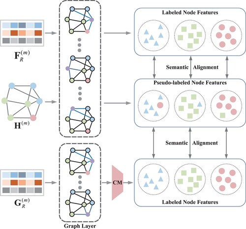
In this section, we propose a Multi-Semantic Aligned Graph Convolutional Network (MSAGCN). The single-layer processing flow of the model is illustrated in Figure 1. The semantic information is first obtained by aggregation from three perspectives of nodes, features, and graph structure, and then aligned by class-centred similarity, which is jointly utilised to solve the problem of over-smoothing and over-fitting of GCN.

Figure 1. Describes the mth layer process of MSAGCN. The three inputs of the convolution layer are ${\mathit{H}}^{(m)}$, ${\mathit{G}}_R^{(m)}$, and ${\mathit{F}}_R^{(m)}$. The three outputs are a pseudo-labelled node feature and two labelled node features. CM in the figure indicates Conversion Module, i.e. ${\mathit{G}}_R^{(m)}$ needs to be transformed after passing through the convolution layer.

4.1. Multi-angle aggregation

MSAGCN has three different inputs to implement multi-angle aggregation operations. The first perspective is graph structure aggregation, i.e. aggregation of features from the graph structure perspective. Given the adjacency matrix $\mathit{A}$ and the identity matrix $\mathit{X}$, the propagation rule can be described as: (4) $\begin{array}{rl}& {\mathit{H}}^{(0)}=\mathit{X}\\ & {\mathit{H}}^{(m+1)}=\sigma \left(\tilde{\mathit{P}}{\mathit{H}}^{(m)}{\mathit{W}}^{(m)}\right)(m=0,1,2,\dots ,M-1)\end{array}$(4) The second perspective is feature aggregation, which is only an aggregation of features from the feature perspective. Given the feature matrix $\mathit{X}$, its propagation rule can be described as: (5) $\begin{array}{rl}& {\mathit{F}}^{(0)}=\mathit{X}\\ & {\mathit{F}}^{(m+1)}=\sigma \left({\mathit{I}}_{\mathit{n}}{\mathit{F}}^{(m)}{\mathit{W}}^{(m)}\right)(m=0,1,2,\dots ,M-1)\end{array}$(5) The third perspective is the node aggregation, i.e. the nodes are aggregated from the feature perspective, and the node features for the current layer are obtained after processing by the CM module. Given a feature matrix $\mathit{X}$, its propagation rule can be described as: (6) $\begin{array}{rl}& {\mathit{G}}^{(0)}={\mathit{X}}^{\mathit{T}}\\ & {\mathit{G}}^{(m+1)}=\sigma \left({\mathit{I}}_{\mathit{g}}{\mathit{G}}^{(m)}{\mathit{Q}}^{(m)}\right)(m=0,1,2,\dots ,M-2)\\ & {\mathit{G}}_{cm}^{(\mathit{m}+\mathbf{1})}=\left(\mathit{A}\mathit{X}\mathit{U}{\mathit{G}}^{(m+1)}\right)(m=0,1,2,\dots ,M-2)\\ & {\mathit{G}}^{(M)}=\sigma \left(\tilde{\mathit{P}}{\mathit{G}}_{cm}^{(\mathit{M}-\mathbf{1})}{\mathit{W}}^{(M-1)}\right)\end{array}$(6) where ${\mathit{I}}_{\mathit{g}}\in {\mathbb{R}}^{d_0\times d_0}$ denotes the identity matrix ($d_0$ indicates the dimensionality of the node features.) and ${\mathit{Q}}^{(m)}\in {\mathbb{R}}^{l_0\times l_{m+1}}$ represents the trainable parameter matrix. ${\mathit{X}}^{\mathit{T}}$ means transposing the feature matrix, and ${\mathit{G}}_{cm}^{(\mathit{m})}$ is the conversion of the feature representation for the corresponding layer to the node representation, where $\mathit{U}\in {\mathbb{R}}^{d_0\times d_0}$ indicates the excess matrix. In addition, when $m\ne 0$, $d_m=l_m$. When m = 0, $d_0$ and $l_0$ represent the feature dimension and the number of nodes, respectively.

In summary, the outputs of MSAGCN are the features ${\mathit{H}}^{(M)}$, ${\mathit{F}}^{(M)}$, and ${\mathit{G}}^{(M)}$, respectively, and the final outputs obtained using softmax activation are ${\mathit{H}}^{\mathrm{out}}=\mathrm{softmax}({\mathit{H}}^{(M)})\in {\mathbb{R}}^{n\times c}$, ${\mathit{F}}^{\mathrm{out}}=\mathrm{softmax}({\mathit{F}}^{(M)})\in {\mathbb{R}}^{n\times c}$, and ${\mathit{G}}^{\mathrm{out}}=\mathrm{softmax}({\mathit{G}}^{(M)})\in {\mathbb{R}}^{n\times c}$. Finally, we train the parameters in the model by minimising the cross-entropy loss, and the loss function can be described as: (7) ${\mathcal{L}}_{Semi}=-\sum _{i\in R}\sum _{k=1}^c({\mathit{Y}}_{ik}\ln {\mathit{H}}_{ik}^{out}+{\mathit{Y}}_{ik}\ln {\mathit{F}}_{ik}^{out}+{\mathit{Y}}_{ik}\ln {\mathit{G}}_{ik}^{out})$(7) where R represents the set of nodes with actual labels. ${\mathit{Y}}_{ik}$ indicates the relationship between node i and label k. If the label of node i is k, then ${\mathit{Y}}_{ik}=1$, otherwise ${\mathit{Y}}_{ik}=0$.

With the increase of stacking layers, the features of nodes become similar or identical after transformation. The second and third terms in ${\mathcal{L}}_{Semi}$ can effectively alleviate this situation by aggregating from three perspectives.

4.2. Semantic alignment

Aggregation is performed from three perspectives: graph structure, features, and nodes, with ${\mathit{H}}^{(m)}$, ${\mathit{F}}^{(m)}$, and ${\mathit{G}}_{cm}^{(m)}$ denoting node features after convolution, respectively. As the convolution of three angles operates on the same feature matrix, we assume that the features of nodes in the same class should be similar after aggregation in the ideal case. In addition, we utilise the same network parameters in the last layer of the model to enable ${\mathit{G}}^{(M)}$ to to obtain guidance from ${\mathit{H}}^{(M)}$ and ${\mathit{F}}^{(M)}$. In conclusion, since neither ${\mathit{F}}^{(m)}$ nor ${\mathit{G}}^{(m)}$ produces over-smoothing when stacking more layers, we adopte ${\mathit{F}}^{(m)}$ and ${\mathit{G}}_{cm}^{(m)}$ as the guiding semantics for ${\mathit{H}}^{(m)}$. Meanwhile, let ${\mathit{F}}_R^{(m)}$ and ${\mathit{G}}_{cm,R}^{(m)}$ denote the semantic information extracted from R and utilise the semantic alignment operation to make the three perspectives semantics of nodes for the same class mapped nearby.

In semi-supervised learning, since the labels of most nodes are unknown, we utilise pseudo-labels to achieve semantic alignment during model training. We adopt the corresponding actual labels for ${\mathit{F}}_R^{(m)}$, ${\mathit{G}}_{cm,R}^{(m)}$ and the nodes with actual labels in ${\mathit{H}}^{(m)}$ as the class information. In contrast, for unlabelled nodes in ${\mathit{H}}^{(m)}$, the MSAGCN model assigns pseudo-labels to the nodes and employs class-centred similarity to alleviate the negative influence of pseudo-labels. The class-centred similarity can be described as: (8) ${\mathcal{L}}_{sema}=\sum _{j=1}^c\{\mathrm{sed}({\mathit{C}}_j\left({\mathit{F}}_R^{(m)}\right),{\mathit{C}}_j\left({\mathit{H}}^{(m)}\right))+\mathrm{sed}({\mathit{C}}_j\left({\mathit{G}}_{cm,R}^{(m)}\right),{\mathit{C}}_j\left({\mathit{H}}^{(m)}\right))\}$(8) where ${\mathit{C}}_j({\mathit{F}}_R^{(m)})$, ${\mathit{C}}_j({\mathit{H}}^{(m)})$, and ${\mathit{C}}_j({\mathit{G}}_{cm,R}^{(m)})$ denote the class-centred of class j belonging to ${\mathit{F}}_R^{(m)}$, ${\mathit{H}}^{(m)}$, and ${\mathit{G}}_{cm,R}^{(m)}$, respectively. The $sed(\cdot )$ function calculates the squared Euclidean distance between matrices. As with X. Yang et al. (2021), we adopt the class-centred alignment to mitigate the noise of ${\mathit{H}}^{(m)}$.

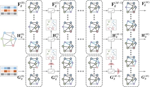
The overall framework of our proposed MSAGCN is illustrated in Figure 2, which utilises three semantic alignments per layer to mitigate the noise during graph propagation to alleviate the over-smoothing problem. In addition, the class-centred similarity for labelled and unlabelled nodes can provide supervised information for the classification task and improve the model's classification performance. The loss function for semantic alignment can be described as: (9) ${\mathcal{L}}_{Sema}=\sum _{m=1}^M\sum _{j=1}^c\{\mathrm{sed}({\mathit{C}}_j\left({\mathit{F}}_R^{(m)}\right),{\mathit{C}}_j\left({\mathit{H}}^{(m)}\right))+\mathrm{sed}({\mathit{C}}_j\left({\mathit{G}}_{cm,R}^{(m)}\right),{\mathit{C}}_j\left({\mathit{H}}^{(m)}\right))\}$(9) Combining the losses of both classification and semantic alignment, we can describe the total objective function as: (10) $\mathcal{L}={\mathcal{L}}_{\mathrm{Semi}}+\lambda {\mathcal{L}}_{\mathrm{Sema}}$(10) In order to improve the stability of the pseudo-label construction class-centred in the classification task, we first compute the respective class-centred ${\mathit{C}}_j({\mathit{F}}_R^{(m)})$, ${\mathit{C}}_j({\mathit{G}}_{cm,R}^{(m)})$, and ${\mathit{C}}_j({\mathit{H}}^{(m)})$ with the current layer features ${\mathit{F}}_R^{(m)}$, ${\mathit{G}}_{cm,R}^{(m)}$, and ${\mathit{H}}^{(m)}$ during each iteration. Then, the class-centred of the last iteration is added to the class-centred of the current layer to ensure stability. This can be described as follows: (11) $\begin{array}{rl}{\mathit{C}}_j^t\left({\mathit{F}}^{(m)}\right)& \leftarrow (1-\alpha ){\mathit{C}}_j^t\left({\mathit{F}}^{(m)}\right)+\alpha {\mathit{C}}_j^{(t-1)}\left({\mathit{F}}^{(m)}\right)\\ {\mathit{C}}_j^t\left({\mathit{H}}^{(m)}\right)& \leftarrow (1-\alpha ){\mathit{C}}_j^t\left({\mathit{H}}^{(m)}\right)+\alpha {\mathit{C}}_j^{(t-1)}\left({\mathit{H}}^{(m)}\right)\\ {\mathit{C}}_j^t\left({\mathit{G}}_{cm,R}^{(m)}\right)& \leftarrow (1-\alpha ){\mathit{C}}_j^t\left({\mathit{G}}_{cm,R}^{(m)}\right)+\alpha {\mathit{C}}_j^{(t-1)}\left({\mathit{G}}_{cm,R}^{(m)}\right)\end{array}$(11) where $\alpha \in [0,1)$ denotes the weighting factor. Finally, MSAGCN algorithm is shown in Algorithm 1.

Figure 2. The overall framework of MSAGCN. We obtain node features by aggregation from three perspectives: graph structure, features, and nodes, and then achieve similar features from the above perspectives layer by layer with semantic alignment.

4.3. Further analysis

The features of a node in the ideal environment can be utilised to determine its class. For the semi-supervised classification task, graph structure-based propagation can pass semantic information from labelled to unlabelled nodes because we assume that neighbouring nodes usually belong to the same class. However, M. Liu et al. (2020) proved that the class of nodes is determined by their features rather than their topology. Therefore, based on X. Yang et al. (2021), we add the filtering of nodes from the perspective of features and then obtain the node features from another perspective by transformation. Finally, we adopt the semantic alignment operation for feature learning during constraint graph propagation.

Moreover, we utilise semantic alignment operations to ensure that all obtained features are similar. In summary, we extract node features from different perspectives and drive all feature distributions to converge, which provides more constraints on node feature learning and improves performance.

5. Experiments

In this section, we will evaluate the performance of the proposed model by conducting extensive experiments on three benchmark citation datasets. In addition, we will provide some visualisations to help illustrate the results.

5.1. Datasets

We evaluate the proposed method on three benchmark citation datasets, including Cora (McCallum et al., 2000), Citeseer (Giles et al., 1998), and Pubmed (Sen et al., 2008). The Citation network represents the citation relationship between documents and documents. Nodes and labels represent documents and their topics. Features of nodes are the bag of words in the document content, and edges represent the mutual references between documents.

• Cora has 5429 edges and 2708 nodes. Seven class labels exist for nodes and 1433-dimensional feature vectors for each node.

• Citeseer has 4732 edges and 3327 nodes. Six class labels exist for nodes and 3707-dimensional feature vectors for each node.

• Pubmed is a more extensive citation network containing 44,338 edges and 19,717 nodes. Three class labels exist for nodes and 400-dimensional feature vectors for each node.

5.2. Baseline

We evaluate the model's performance in two aspects, so the baselines are divided into two categories. The first category is that the number of labelled nodes is severely scarce, and the second category is that stacking multiple layers leads to an over-smoothing phenomenon.

Category 1: the number of labelled nodes is severely scarce.

• GCN (Kipf & Welling, 2016) performs feature transformation by matrix mapping and node aggregation with pooling functions.

• GAT (Veličković et al., 2017) aggregates neighbouring nodes through a self-attention mechanism to achieve personalised weights.

• SGC (Wu et al., 2019) captures information of higher order in a graph by taking the Kth power of the graph convolution matrix.

• APPNP (Klicpera et al., 2018) combines PageRank with GCN to solve the limited range problem in the messaging model.

• ICGN (Q. Li et al., 2019) takes graph similarity as a signal on the graph and utilises low-pass graph filters to extract helpful data representations for classification.

• DAGNN (M. Liu et al., 2020) decouples feature transformation and propagation entanglement, allowing deep graph neural networks to utilise a sizeable receptive domain without causing performance degradation.

• Shoestring (Lin et al., 2020) combines metric learning into a semi-supervised learning paradigm for graphs.

• SelfSAGCN (X. Yang et al., 2021) learns the features of nodes from the same class in terms of both graph structure and semantics and maps nearby.

Category 2: stacking multiple layers leads to an over-smoothing phenomenon.

• DropEdge (Rong et al., 2019) randomly removes random edges from the graph to reduce the convergence speed of over-smoothing.

• ResGCN (G. Li et al., 2019) borrows from CNN by introducing residual/dense connectivity and dilation convolution to build deep convolutional networks.

• JKNet (Xu et al., 2018) proposes jumping knowledge networks (JK), allowing each node to exploit different neighbourhood ranges flexibly to achieve a better structure-aware representation.

• IncepGCN (Rong et al., 2019) extends convolutional networks by decomposing convolution and regularisation.

• GCNII (Chen et al., 2020) is an extension of vanilla GCN that utilises identity mapping and initial residuals to mitigate the over-smoothing problem.

• SelfSAGCN (X. Yang et al., 2021) learns the features of nodes from the same class in terms of both graph structure and semantics and maps nearby.

5.3. Setup

Our implementation of MSAGCN uses Pytorch¹ and adopts the public code of SelfSAGCN (X. Yang et al., 2021).² Our method's parameter settings are identical to those of SelfSAGCN (X. Yang et al., 2021) to ensure the comparison's fairness for the experimental results. We employ the Adam optimiser, with the learning rate set to 0.01, the dropout set to 0.5, the weight decay set to $5\mathrm{e}-4$, and the class-centred weighting factor set to 0.7. The λ ($\lambda \leftarrow \lambda (\frac{2}{1+{\mathrm{e}}^{-10\times p}}-1)$) is taken to mitigate the noise of pseudo-labels in the early stage of training, where p denotes the training period.

5.4. Performance comparison

We evaluated the performance of MSAGCN in the usual case (i.e. 20 labelled nodes per class). As shown in Table 2, our model performs relatively well in the usual case.

Table 2. Classification accuracy (%) for 20 labelled nodes per class.

Method	Cora	Citeseer	Pubmed
MLP	$61.6\pm 0.2$	$61.0\pm 0.3$	$74.2\pm 0.2$
GCN (Kipf & Welling, 2016)	$81.2\pm 0.4$	$71.1\pm 0.7$	$78.5\pm 1.0$
GAT (Veličković et al., 2017)	$83.1\pm 0.7$	$70.8\pm 0.9$	$71.1\pm 1.2$
APPNP (Klicpera et al., 2018)	$83.3\pm 2.4$	$71.8\pm 0.9$	$80.1\pm 1.3$
SGC (Wu et al., 2019)	$81.7\pm 0.6$	$71.3\pm 1.1$	$78.9\pm 1.3$
Shoestring (Lin et al., 2020)	$81.9\pm 2.1$	$69.5\pm 2.4$	$79.7\pm 4.5$
DAGNN (M. Liu et al., 2020)	$\mathbf{84.4}\pm 0.4$	$73.3\pm 0.7$	$80.5\pm 0.9$
SelfSAGCN (X. Yang et al., 2021)	$83.8\pm 0.5$	$73.5\pm 1.2$	$\mathbf{80.7}\pm 1.5$
MSAGCN	$84.0\pm 0.6$	$\mathbf{73.8}\pm 0.9$	$80.5\pm 1.2$

5.5. Model performance when labelled nodes are severely sparse

In this section, we evaluate the performance of MSAGCN under a severe scarcity of labelled nodes. Table 3 shows the performance of various models with 1, 2, and 5 labelled nodes per class, respectively.

Table 3. Classification accuracy (%) for the severe scarcity of labelled nodes per class on three datasets.

	1-label			2-label			5-label
Method	Cora	Citeseer	Pubmed	Cora	Citeseer	Pubmed	Cora	Citeseer	Pubmed
GCN (Kipf & Welling, 2016)	$43.1\pm 0.7$	$29.2\pm 0.9$	$51.5\pm 1.8$	$58.0\pm 0.6$	$40.5\pm 0.7$	$60.4\pm 2.3$	$69.1\pm 0.5$	$53.7\pm 0.9$	$68.4\pm 3.2$
GAT (Veličković et al., 2017)	$45.2\pm 0.6$	$32.5\pm 1.0$	$53.5\pm 2.3$	$59.7\pm 0.4$	$43.2\pm 0.7$	$62.2\pm 2.2$	$70.2\pm 0.3$	$55.2\pm 0.7$	$69.5\pm 1.1$
APPNP (Klicpera et al., 2018)	$45.2\pm 0.3$	$33.5\pm 1.2$	$52.3\pm 3.2$	$58.3\pm 0.7$	$50.1\pm 0.6$	$62.7\pm 1.3$	$71.2\pm 0.5$	$55.9\pm 0.9$	$70.7\pm 1.3$
SGC (Wu et al., 2019)	$44.5\pm 0.5$	$31.4\pm 0.9$	$55.2\pm 2.3$	$58.6\pm 0.5$	$45.8\pm 0.6$	$63.5\pm 2.9$	$69.5\pm 0.4$	$54.6\pm 0.8$	$71.4\pm 2.9$
ICGN (Q. Li et al., 2019)	$43.3\pm 0.5$	$35.0\pm 1.1$	$54.2\pm 1.5$	$63.5\pm 2.7$	$43.9\pm 1.9$	$62.6\pm 3.2$	$72.2\pm 2.5$	$55.9\pm 0.9$	$70.7\pm 1.3$
DAGNN (M. Liu et al., 2020)	$59.2\pm 0.4$	$45.2\pm 0.7$	$58.5\pm 2.4$	$65.6\pm 0.8$	$54.3\pm 0.8$	$65.3\pm 2.7$	$72.0\pm 0.4$	$58.1\pm 0.9$	$71.4\pm 2.2$
Shoestring (Lin et al., 2020)	$60.2\pm 0.9$	$52.2\pm 1.3$	$60.3\pm 6.1$	$68.3\pm 0.9$	$60.1\pm 1.3$	$63.5\pm 5.7$	$73.0\pm 1.2$	$64.2\pm 1.5$	$68.4\pm 6.3$
SelfSAGCN (X. Yang et al., 2021)	$63.5\pm 0.8$	$57.5\pm 3.7$	$65.0\pm 3.3$	$71.7\pm 0.6$	$68.3\pm 1.2$	$\mathbf{70.9}\pm 1.9$	$75.1\pm 0.7$	$71.9\pm 1.3$	$\mathbf{73.0}\pm 2.1$
MSAGCN	$\mathbf{65.2}\pm 0.7$	$\mathbf{60.1}\pm 2.1$	$\mathbf{67.7}\pm 2.2$	$\mathbf{73.1}\pm 0.5$	$\mathbf{69.5}\pm 1.7$	$70.7\pm 1.7$	$\mathbf{77.4}\pm 0.5$	$\mathbf{72.8}\pm 1.1$	$72.8\pm 1.6$

Table 3 shows the following observations:

• When labelled nodes are extremely rare, MSAGCN outperforms the baselines methods on the three benchmark datasets.

• Compared with the results of SelfSAGCN, MSAGCN does obtain better results. It illustrates that the aggregation from the third perspective can improve the learning ability of the model.

• The performance improvement is most significant when only one labelled node per class.

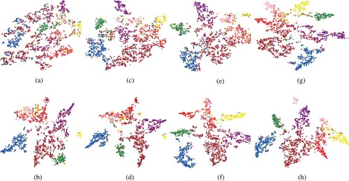
From these observations, it can be concluded that MSAGCN performs well when labelled nodes are severely scarce. When labelled nodes are severely scarce, aggregating features from different perspectives and aligning semantics could reinforce the similar parts and help improve the learning ability of the model. In addition, we visualise the distribution of different numbers of labelled node features on the Cora dataset in Figure 3 with t-SNE (Van der Maaten & Hinton, 2008) for better observation.

Figure 3. We employ different colours to identify different classes to visualise the discriminative capability of node features on the Cora dataset. The upper and lower parts represent the visualisation results of GCN and MSAGCN, respectively. (a) GCN:1-label. (b) MSAGCN:1-label. (c) GCN:2-label. (d) MSAGCN:2-label. (e) GCN:5-label. (f) MSAGCN:5-label. (g) GCN:20-label and (h) MSAGCN:20-label.

5.6. Model performance with different numbers of labelled nodes

For the completeness of the experiment, we evaluate the model's performance with various numbers of labelled nodes. Figure 4 illustrates the results in more detail.

Figure 4. Model performance with various numbers of labelled nodes.

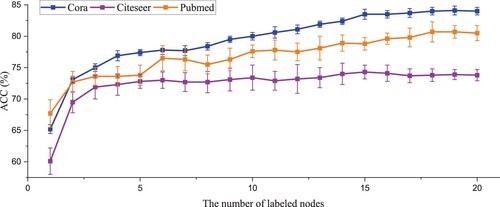
From Figure 4, we have the following observations:

• The performance increases significantly for both Cora and Pubmed datasets as the number of labelled nodes increases.

• The model performance improves dramatically as the number of labelled nodes per class increases from 1 to 2 in the Citeseer dataset. However, the performance increase is relatively small when the number of labelled nodes per class increases from 2 to 20.

From these observations, it can be concluded that MSAGCN performs well when labelled nodes are severely scarce. In addition, the model has relatively poor performance improvement on the Citeseer dataset due to its sizeable feature-to-node ratio, i.e. each feature corresponds to relatively few nodes.

5.7. Parameter analysis

In this section, we analyse the parameters in MSAGCN. Figure 5(a,b) show the influence of two hyperparameters on the model performance.

Figure 5. Influence of different hyperparameters on model performance. (a) Model performance with various balance weights $\mathit{\alpha }$ on the Cora dataset. (b) Model performance with various loss balance weights $\mathit{\lambda }$ on the Cora dataset. (a) $\mathit{\alpha }$ and (b) $\mathit{\lambda }$.

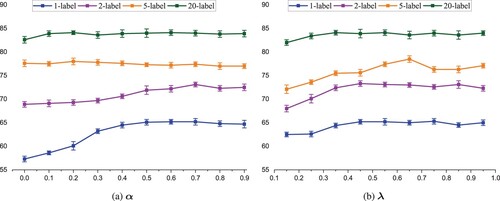
Figure 5 shows the following observations:

• Our model is not sensitive to $\mathit{\alpha }$ within the range $[0.3,0.9]$ based on investigating different balance weights alpha in Figure 5(a).

• Once the lambda exceeds 0.55 in a two-layer model, the parameter $\mathit{\lambda }$ has little effect on model performance in Figure 5(b).

• As shown in Figure 5, our model's performance is insensitive to the two hyperparameters when there are more labelled nodes per class.

5.8. model performance with multiple layers

In this section, we evaluate the performance results of the model with different hidden layers. Table 4 shows the model's performance with different numbers of hidden layers, the same as the SelfSAGCN setup, where we apply 20 labelled nodes per class for training.

Table 4. Classification accuracy (%) of the model on the three benchmark datasets with various numbers of layers.

	4-Layer			8-Layer			16-Layer
Method	Cora	Citeseer	Pubmed	Cora	Citeseer	Pubmed	Cora	Citeseer	Pubmed
GCN (Kipf & Welling, 2016)	$80.4\pm 0.4$	$67.6\pm 0.9$	$79.0\pm 1.2$	$69.5\pm 0.1$	$30.2\pm 0.3$	$61.2\pm 1.5$	$64.9\pm 1.4$	$18.3\pm 1.1$	$40.9\pm 0.7$
GCNdrop (Rong et al., 2019)	$82.0\pm 0.7$	$70.2\pm 0.8$	$79.1\pm 1.4$	$75.8\pm 0.4$	$61.4\pm 0.5$	$78.1\pm 0.7$	$75.7\pm 1.1$	$57.2\pm 0.9$	$78.5\pm 1.5$
JKNet (Xu et al., 2018)	$80.2\pm 0.5$	$68.7\pm 0.4$	$78.0\pm 1.0$	$80.7\pm 0.6$	$67.7\pm 0.3$	$78.1\pm 1.4$	$80.2\pm 1.0$	$69.8\pm 0.7$	$72.6\pm 1.4$
IncepGCN (Rong et al., 2019)	$77.6\pm 0.5$	$69.3\pm 0.6$	$77.0\pm 0.7$	$76.5\pm 0.8$	$68.4\pm 0.5$	$77.9\pm 1.2$	$81.7\pm 0.7$	$70.2\pm 0.9$	$74.9\pm 1.7$
ResGCN (G. Li et al., 2019)	$78.8\pm 0.6$	$70.5\pm 0.6$	$78.6\pm 1.5$	$75.6\pm 0.5$	$65.0\pm 0.4$	$78.1\pm 1.3$	$72.0\pm 0.8$	$66.5\pm 0.5$	$75.5\pm 1.0$
DAGNN (M. Liu et al., 2020)	$82.1\pm 0.5$	$68.5\pm 0.9$	$77.5\pm 0.9$	$83.2\pm 0.6$	$70.2\pm 0.4$	$78.4\pm 0.9$	$81.7\pm 0.8$	$68.4\pm 0.9$	$79.8\pm 1.0$
GCNII (Chen et al., 2020)	$82.0\pm 0.4$	$68.7\pm 0.4$	$78.6\pm 0.4$	$\mathbf{84.1}\pm 0.3$	$70.6\pm 0.5$	$\mathbf{79.4}\pm 0.6$	$\mathbf{84.6}\pm 0.8$	$\mathbf{72.9}\pm 0.9$	$\mathbf{80.2}\pm 1.0$
SelfSAGCN (X. Yang et al., 2021)	$82.3\pm 0.3$	$\mathbf{72.3}\pm 0.8$	$\mathbf{79.5}\pm 1.2$	$81.9\pm 0.5$	$71.0\pm 1.1$	$78.7\pm 1.3$	$80.5\pm 0.3$	$68.0\pm 1.2$	$78.1\pm 1.4$
MSAGCN	$\mathbf{83.0}\pm 0.6$	$\mathbf{72.3}\pm 0.6$	$79.3\pm 0.9$	$82.4\pm 0.7$	$\mathbf{71.3}\pm 0.8$	$78.0\pm 1.5$	$82.1\pm 0.5$	$68.9\pm 0.9$	$77.3\pm 1.3$

According to Table 4, we can observe that our algorithm performs best when we apply the 4-layer model. The results illustrate that our proposed model can strengthen the similar parts by aggregating features from different perspectives and aligning the semantics, which can partly alleviate the over-smoothing problem.

5.9. Limitations

In this section, we will discuss some of the limitations that exist in the model.

Rich information contained in the connection The current model of multi-angle extraction of features focuses only on whether the feature is included and ignores other important information, such as the frequency of feature occurrence. In addition, extracting the semantic information in a node from the feature perspective focuses only on whether the node is possessed or not, and ignores the structural information between nodes, i.e. ignores the potential nodes contained in the feature.

Feature-to-feature interaction The model considers the existence of cross-reference relationships between nodes and ignores the possibility of some relationship between features. For example, the features indicate similar or opposite meanings and the size of the range of features.

6. Conclusion

In this paper, we propose a Multi-Semantic Alignment Graph Convolutional Network (MSAGCN) to address the issues of over-fitting and over-smoothing. The method extracts semantic information from labelled nodes layer by layer with multi-angle aggregation operation and then processes the obtained node features by semantic alignment operation, effectively alleviating the over-fitting and over-smoothing of GCN. The proposal of MSAGCN has promoted the development and application of network topology research. In addition, we build the class-centred for unlabelled nodes with assigned pseudo-labels and gradually revise them to mitigate noise. As a result, the node features extracted from different angles are forced to converge, resulting in improved node classification. We evaluate the model on three benchmark datasets, demonstrating that our method outperforms SOTA methods on classification tasks. In the future, we will apply the method of MSAGCN to heterogeneous graphs, where the multi-angle aggregation is easier to find vital features in heterogeneous relationships.

Disclosure statement

No potential conflict of interest was reported by the author(s).

Correction Statement

This article was originally published with errors, which have now been corrected in the online version. Please see Correction http://dx.doi.org/10.1080/09540091.2022.2130588

Additional information

Funding

This work was supported by the Postgraduate Research & Practice Innovation Program of Jiangsu Province (KYCX21_0484).

Notes

1 https://pytorch.org

2 https://github.com/xdxuyang/SelfSAGCN

References

- Atwood, J., & Towsley, D. (2016). Diffusion-convolutional neural networks. Advances in neural information processing systems (Vol. 29). Curran Associates, Inc.
- Bian, T., Xiao, X., Xu, T., Zhao, P., Huang, W., Rong, Y., & Huang, J. (2020). Rumor detection on social media with bi-directional graph convolutional networks. In Proceedings of the AAAI conference on artificial intelligence (Vol. 34, No. 01, pp. 549–556). https://doi.org/10.1609/aaai.v34i01.5393
- Bruna, J., Zaremba, W., Szlam, A., & LeCun, Y. (2013). Spectral networks and locally connected networks on graphs. arXiv preprint arXiv:1312.6203. https://doi.org/10.48550/arXiv.1312.6203
- Chang, F., Ge, L., Li, S., Wu, K., & Wang, Y. (2021). Self-adaptive spatial-temporal network based on heterogeneous data for air quality prediction. Connection Science, 33(3), 427–446. https://doi.org/10.1080/09540091.2020.1841095
- Chen, M., Wei, Z., Huang, Z., Ding, B., & Li, Y. (2020). Simple and deep graph convolutional networks. In International Conference on Machine Learning (pp. 1725–1735). PMLR.
- Defferrard, M., Bresson, X., & Vandergheynst, P. (2016). Convolutional neural networks on graphs with fast localized spectral filtering. Advances in neural information processing systems (Vol. 29). Curran Associates, Inc.
- Donnat, C., Zitnik, M., Hallac, D., & Leskovec, J. (2018). Learning structural node embeddings via diffusion wavelets. In Proceedings of the 24th ACM SIGKDD international conference on knowledge discovery & data mining (pp. 1320–1329). Association for Computing Machinery. https://doi.org/10.1145/3219819.3220025.
- Feng, F., He, X., Zhang, H., & Chua, T. S. (2021). Cross-GCN: Enhancing graph convolutional network with k-Order feature interactions. IEEE Transactions on Knowledge and Data Engineering. https://doi.org/10.1109/TKDE.2021.3077524
- Giles, C. L., Bollacker, K. D., & Lawrence, S. (1998). CiteSeer: An automatic citation indexing system. In Proceedings of the third ACM conference on digital libraries (pp. 89–98). Association for Computing Machinery.
- Hamilton, W., Ying, Z., & Leskovec, J. (2017). Inductive representation learning on large graphs. In Advances in neural information processing systems (Vol. 30). Curran Associates, Inc.
- Hu, J., Wang, Z., Chen, J., & Dai, Y. (2021). A community partitioning algorithm based on network enhancement. Connection Science, 33(1), 42–61. https://doi.org/10.1080/09540091.2020.1753172
- Hu, N., Zhang, D., Xie, K., Liang, W., & Hsieh, M. Y. (2021). Graph learning-based spatial-temporal graph convolutional neural networks for traffic forecasting. Connection Science, 34(1), 429–448. https://doi.org/10.1080/09540091.2021.2006607.
- Kipf, T. N., & Welling, M. (2016). Semi-supervised classification with graph convolutional networks. arXiv preprint arXiv:1609.02907. https://doi.org/10.48550/arXiv.1609.02907
- Klicpera, J., Bojchevski, A., & Günnemann, S. (2018). Predict then propagate: Graph neural networks meet personalized pagerank. arXiv preprint arXiv:1810.05997. https://doi.org/10.48550/arXiv.1810.05997
- Klicpera, J., Weißenberger, S., & Günnemann, S. (2019). Diffusion improves graph learning. arXiv preprint arXiv:1911.05485. https://doi.org/10.48550/arXiv.1911.05485
- Li, G., Muller, M., Thabet, A., & Ghanem, B. (2019). Deepgcns: Can GCNs go as deep as CNNs ?. In Proceedings of the IEEE/CVF international conference on computer vision (pp. 9267–9276). IEEE.
- Li, J. H., Huang, L., Wang, C. D., Huang, D., Lai, J. H., & Chen, P. (2021). Attributed network embedding with micro-meso structure. ACM Transactions on Knowledge Discovery from Data (TKDD), 15(4), 1–26. https://doi.org/10.1145/3441486
- Li, Q., Han, Z., & Wu, X. M. (2018). Deeper insights into graph convolutional networks for semi-supervised learning. In Thirty-second AAAI conference on artificial intelligence. AAAI press.
- Li, Q., Wu, X. M., Liu, H., Zhang, X., & Guan, Z. (2019). Label efficient semi-supervised learning via graph filtering. In Proceedings of the IEEE/CVF conference on computer vision and pattern recognition (pp. 9582–9591). IEEE.
- Lin, W., Gao, Z., & Li, B. (2020). Shoestring: Graph-based semi-supervised classification with severely limited labeled data. In Proceedings of the IEEE/CVF conference on computer vision and pattern recognition (pp. 4174–4182). IEEE.
- Liu, M., Gao, H., & Ji, S. (2020). Towards deeper graph neural networks. In Proceedings of the 26th ACM SIGKDD international conference on knowledge discovery & data mining (pp. 338–348). Association for Computing Machinery. https://doi.org/10.1145/3394486.3403076.
- Liu, M., Wang, Z., & Ji, S. (2021). Non-local graph neural networks. IEEE Transactions on Pattern Analysis and Machine Intelligence. https://doi.org/10.1109/TPAMI.2021.3134200
- Liu, Z., Huang, C., Yu, Y., & Dong, J. (2021). Motif-preserving dynamic attributed network embedding. In Proceedings of the web conference 2021 (pp. 1629–1638). Association for Computing Machinery. https://doi.org/10.1145/3442381.3449821.
- McCallum, A. K., Nigam, K., Rennie, J., & Seymore, K. (2000). Automating the construction of internet portals with machine learning. Information Retrieval, 3(2), 127–163. https://doi.org/10.1023/A:1009953814988
- Mishra, P., Del Tredici, M., Yannakoudakis, H., & Shutova, E. (2019). Abusive language detection with graph convolutional networks. arXiv preprint arXiv:1904.04073. https://doi.org/10.48550/arXiv.1904.04073
- Monti, F., Boscaini, D., Masci, J., Rodola, E., Svoboda, J., & Bronstein, M. M. (2017). Geometric deep learning on graphs and manifolds using mixture model CNNs. In Proceedings of the IEEE conference on computer vision and pattern recognition (pp. 5115–5124). IEEE.
- Pan, G., Yao, Y., Tong, H., Xu, F., & Lu, J. (2021). Unsupervised attributed network embedding via cross fusion. . In Proceedings of the 14th ACM international conference on web search and data mining (pp. 797–805). Association for Computing Machinery. https://doi.org/10.1145/3437963.3441763.
- Pei, H., Wei, B., Chang, K. C. C., Lei, Y., & Yang, B. (2020). Geom-GCN: Geometric graph convolutional networks. arXiv preprint arXiv:2002.05287. https://doi.org/10.48550/arXiv.2002.05287
- Qin, J., Zeng, X., Wu, S., & Tang, E. (2021). E-GCN: Graph convolution with estimated labels. Applied Intelligence, 51(7), 5007–5015. https://doi.org/10.1007/s10489-020-02093-5
- Qin, J., Zeng, X., Wu, S., & Zou, Y. (2022). Feature recommendation strategy for graph convolutional network. Connection Science, 34(1), 1697–1718. https://doi.org/10.1080/09540091.2022.2080806
- Rong, Y., Huang, W., Xu, T., & Huang, J. (2019). Dropedge: Towards deep graph convolutional networks on node classification. arXiv preprint arXiv:1907.10903. https://doi.org/10.48550/arXiv.1907.10903
- Sen, P., Namata, G., Bilgic, M., Getoor, L., Galligher, B., & Eliassi-Rad, T. (2008). Collective classification in network data. AI Magazine, 29(3), 93–93. https://doi.org/10.1609/aimag.v29i3.2157
- Song, X., Li, J., Lei, Q., Zhao, W., Chen, Y., & Mian, A. (2022). Bi-CLKT: Bi-graph contrastive learning based knowledge tracing. Knowledge-Based Systems, 241(C), 108247–108247.
- Song, X., Li, J., Tang, Y., Zhao, T., Chen, Y., & Guan, Z. (2021). Jkt: A joint graph convolutional network based deep knowledge tracing. Information Sciences, 580(C), 510–523. https://doi.org/10.1016/j.ins.2021.08.100.
- Tan, Z., Yang, Y., Wan, J., Guo, G., & Li, S. Z. (2020). Relation-aware pedestrian attribute recognition with graph convolutional networks. In Proceedings of the AAAI conference on artificial intelligence (Vol. 34, No. 07, pp. 12055–12062). AAAI Press. https://doi.org/10.1609/aaai.v34i07.6883.
- Van der Maaten, L., & Hinton, G. (2008). Visualizing data using t-SNE. Journal of Machine Learning Research, 9(11), 2579–2605.
- Veličković, P., Cucurull, G., Casanova, A., Romero, A., Lio, P., & Bengio, Y. (2017). Graph attention networks. arXiv preprint arXiv:1710.10903. https://doi.org/10.48550/arXiv.1710.10903
- Wang, H., Lian, D., & Ge, Y. (2019). Binarized collaborative filtering with distilling graph convolutional networks. arXiv preprint arXiv:1906.01829. https://doi.org/10.48550/arXiv.1906.01829
- Wu, F., Souza, A., Zhang, T., Fifty, C., Yu, T., & Weinberger, K. (2019). Simplifying graph convolutional networks. In International conference on machine learning (pp. 6861–6871). PMLR.
- Xu, K., Li, C., Tian, Y., Sonobe, T., Kawarabayashi, K. I., & Jegelka, S. (2018). Representation learning on graphs with jumping knowledge networks. In International conference on machine learning (pp. 5453–5462). PMLR.
- Xu, K., Li, J., Zhang, M., Du, S. S., Kawarabayashi, K. I., & Jegelka, S. (2019). What can neural networks reason about?. arXiv preprint arXiv:1905.13211. https://doi.org/10.48550/arXiv.1905.13211
- Yang, L., Kang, Z., Cao, X., Jin, D., Yang, B., & Guo, Y. (2019). Topology optimization based graph convolutional network. In IJCAI (pp. 4054–4061). AAAI Press.
- Yang, X., Deng, C., Dang, Z., Wei, K., & Yan, J. (2021). SelfSAGCN: Self-supervised semantic alignment for graph convolution network. In Proceedings of the IEEE/CVF conference on computer vision and pattern recognition (pp. 16775–16784). IEEE.
- Yang, Y., Guan, Z., Li, J., Zhao, W., Cui, J., & Wang, Q. (2021). Interpretable and efficient heterogeneous graph convolutional network. IEEE Transactions on Knowledge and Data Engineering. https://doi.org/10.1109/TKDE.2021.3101356
- Zhao, C., Li, X., Shao, Z., Yang, H., & Wang, F. (2022). Multi-featured spatial-temporal and dynamic multi-graph convolutional network for metro passenger flow prediction. Connection Science, 34(1), 1252–1272. https://doi.org/10.1080/09540091.2022.2061915
- Zhu, Q., Du, B., & Yan, P. (2020). Self-supervised training of graph convolutional networks. arXiv preprint arXiv:2006.02380. https://doi.org/10.48550/arXiv.2006.02380