WAM to SeeSaw model for cancer therapy – overcoming LQM difficulties –

Abstract

Purpose

The assessment of biological effects caused by radiation exposure has been currently carried out with the linear-quadratic (LQ) model as an extension of the linear non-threshold (LNT) model. In this study, we suggest a new mathematical model named as SeaSaw (SS) model, which describes proliferation and cell death effects by taking account of Bergonie-Tribondeau’s law in terms of a differential equation in time. We show how this model overcomes the long-standing difficulties of the LQ model.

Materials and methods

We construct the SS model as an extended Wack-A-Mole (WAM) model by using a differential equation with respect to time in order to express the dynamics of the proliferation effect. A large number of accumulated data of such parameters as α and β in the LQ based models provide us with valuable pieces of information on the corresponding parameter $b_1$ and the maximum volume $V_m$ of the SS model. The dose rate $b_1$ and the notion of active cell can explain the present data without introduction of β, which is obtained by comparing the SS model with not only the cancer therapy data but also with in vitro experimental data. Numerical calculations are presented to grasp the global features of the SS model.

Results

The SS model predicts the time dependence of the number of active- and inactive-cells. The SS model clarifies how the effect of radiation depends on the cancer stage at the starting time in the treatment. Further, the time dependence of the tumor volume is calculated by changing individual dose strength, which results in the change of the irradiation duration for the same effect. We can consider continuous irradiation in the SS model with interesting outcome on the time dependence of the tumor volume for various dose rates. Especially by choosing the value of the dose rate to be balanced with the total growth rate, the tumor volume is kept constant.

Conclusions

The SS model gives a simple equation to study the situation of clinical radiation therapy and risk estimation of radiation. The radiation parameter extracted from the cancer therapy is close to the value obtained from animal experiment in vitro and in vivo. We expect the SS model leads us to a unified description of radiation therapy and protection and provides a great development in cancer-therapy clinical-planning.

Keywords:

• SeeSaw model
• WAM
• LQM
• radiotherapy
• dose rate
• risk estimation

1. Introduction

The study of radio-biology started just after the discovery of radioactivity in 1896. Scientists at that time assessed biological effects caused by radiation exposure from positive and negative aspects (Bodgi et al. 2016). For the former point, Pierre Curie was curious enough to wrap radioactive material around his arm and confirmed the appearance of erythema. He came up with the idea that if it can kill cells, it is possible to kill cancer cells also, and proposed a cancer therapy project. On the other hand, as for the latter point, although the earliest observation was the onset of such obvious effects as skin ulcerations that appeared after intense radiation exposure, it took a little while until they realized the delayed effects such as cancer. As for the construction of a mathematical model for the biological effect induced by radiation exposure, the original idea had already been proposed in the early stage of the history in terms of the so-called target theory by M. Curie (1929). She analyzed the data of Holweck and his group on the effect of X-ray on bacteria and all these authors proposed the basis of the so-called quantum radiobiology (Bodgi et al. 2016). The essence of the target theory is that radiation is absorbed as a quantum by a ‘target’ named as a ‘sensitive zone’ in a cell, yielding damage and eventually cell death.

In 1946, Lea proposed the ‘hit model’ based on the concept of the target theory (Lea 1946), and its predictions were consistent with the observed Drosophila data, namely ‘mutation frequency F increases linearly with total dose’, which is nowadays called ‘linear non-threshold (LNT)’ model.

Now, we should make an important comment that the two phenomena; mutation (Muller 1927) and cell death (Curie 1929), are to be distinguished by the choices of ‘target’; for the case of mutation, the target is a specific locus, and for cell death, the target may be not only a considerable amount of loci but also various kinds of contents in and around cell. This difference results in a huge order of difference in respective biological sensitivities. Lea already had been aware of the experimental fact that the mutation rate caused by irradiation was sometimes reduced with increase of the interval non-irradiation time (Lea 1946), which was later named as ‘Elkind recovery effect’ (Elkind et al. 1964). He added this effect using irradiation intensity per minute, which is nowadays called ‘dose rate’, and introduced a quantity G (GIS) (Lea 1946), which is called as ‘Lea-Catcheside Dose-protraction factor’ (O’Rourke et al. 2009). This factor takes into account the time dependent structure to recognize the essence of the mechanism. We should always consider various effects, which are constantly operating to repair or proliferate cells in living system.

We have proposed the Wack-A-Mole (WAM) model (Manabe et al. 2012; Bando et al. 2017, 2019) to express the above features for the unified description of mutation in various animals including fruit-fly, and even plants (Nakamura et al. 2014; Manabe et al. 2015; Wada et al. 2016) and eventually mouse in the mega-mouse experiment (Manabe and Bando 2013; Tsunoyama et al. 2019). The WAM model describes not only the excess effect of mutation but also the endogenous mutation frequency, which is closely related to the evolution of life (Nakamura et al. 2014). Although they are restricted to focus on the mutation of germ cells, the WAM clarifies how the radiation effects can express the biological effects correctly and simply, if we use a differential equation in time with the above-mentioned increase and decrease mechanisms (Nakamura et al. 2014; Bando et al. 2019) and how the model can estimate the effects of low dose radiation as seen in Fukushima (Wada et al. 2016; Bando et al. 2019).

To describe both the growth and death effects and their interplay, we need a dynamical model that correctly describes the time development. The WAM model as proposed to overcome the deficiency of the LQ model, taking account of the time development of both increase and decrease contributions, most of which are more or less related to cell death mechanism (Galluzzi et al. 2018). Especially, we should distinguish the mutation and cell death processes, which are expressed in terms of two different reaction rates. They are always operating simultaneously in the living biological body. With all the necessary information in hand, we can extend the WAM model to construct a SeeSaw (SS) model, by taking account of an additional process due to proliferation of cancer cells. The proliferation of cancer cells is usually observed in most living cells and is especially needed to apply to the case of cancer therapy.

This paper is arranged as follows. After a quick review of the essence of the WAM model, with the observed values of their dynamical parameters obtained by the mega-mouse experiments in Section 2, we further extend it to the SS model for the cancer cell system which provides us with important tool of radiotherapy in Section 3. We present characteristic features of the SS model in Section 4 and provide numerical results compared with experimental data by picking up some examples in Section 5. Section 6 and 7 are devoted to the conclusion and discussions.

2. WAM in terms of general expression of cell system

Let us explain here a general expression of stimulus-response relation to get the time dependence of the number of cells of the type of interest in the system (organ or tissue) with its number, $N\left(t\right).$ The essence of the present model is to take account of the fate of the number of cells of interest, which is controlled by the biological dynamics. Here, it is important to describe such ever-changing behavior in response to various types of stimuli that cause increase and decrease effects. Namely, the dynamical equation should be expressed in terms of the sum of such stimuli and the simplest expression is written in terms of differential equation with respect to time as, (1) $$\frac{dN\left(t\right)}{dt}=A\overline{N}\left(t\right)+\mathrm{B}N\left(t\right),$$(1) where $\overline{N}\left(t\right)$ is the number of another kind of cells, which is to be distinguished from the cells under consideration expressed by $N\left(t\right).$

If we consider a case, where $N\left(t\right)$ is the number of mutated cells, $\overline{N}\left(t\right)$ is the number of normal cells, which are to be mutated with the reaction rare A, while at the same time the mutated cells are excluded with the reaction rate B and $N\left(t\right)$ decreases due to cell death. Note that the biological system has such an exclusive function, most of which may be apoptosis by which mutated cells are removed frequently with the coefficient B, which should be a negative number. Thus $N\left(t\right)$ is determined as a result of such a seesaw game. These processes are always under operation in living organisms even if there is no external stimulus; we call such process as ‘endogenous mutation’.

The WAM model considers the steady-state without any external stimuli, where the system (tissue or organ) is almost filled by normal cells with its maximal number $N_{\max }.$ Thus, $\overline{N}\left(t\right)$ is almost constant. Namely, we can approximate $\overline{N}\left(t\right)={\overline{N}}_{\max },$ since in the steady-state the ratio of the numbers of mutated and normal cells are of order 10⁻⁵ (Russell and Kelly 1982a). Therefore, we have the following equation for the number of mutated cells. We change the sign of B in the following in order to make clear that B represents the decrease effect. (2) $$\frac{dN\left(t\right)}{dt}\simeq A{\overline{N}}_{\max }-BN\left(t\right) \to \frac{dF\left(t\right)}{dt}=A-BF\left(t\right),\mathrm{ }$$(2) where (3) $$F\left(t\right)\equiv \frac{N\left(t\right)}{{\overline{N}}_{\max }}.$$(3) $\text{We define }F\left(t\right)$ as mutation frequency, and the parameters, A and B, represent the reaction rates from normal cells to mutated cells (increase part of $F\left(t\right)$) and the annihilation rate of mutated cells due to cell death (decrease part of $F\left(t\right)$), respectively.

Again we would like to stress that the above equation is quite different from the original Lea's hit model where it does not have the B term; we have added a decrease term B to account for the effects to reduce $F\left(t\right)$ in the differential equation. Mutated cells are produced with the coefficient A from the normal cells, while they are excluded with the coefficient B by the cell death process.

The dynamical equation of the WAM model in Equation (2)(2) $$\frac{dN\left(t\right)}{dt}\simeq A{\overline{N}}_{\max }-BN\left(t\right) \to \frac{dF\left(t\right)}{dt}=A-BF\left(t\right),\mathrm{ }$$(2) is expressed in terms of a differential equation describing the stimulus-response relationship. In order to include the biological effects caused by radiation exposure, it is natural to introduce external stimuli by adding the radiation terms to the endogenous terms in A and B as, (4) $$A=a_0+a_{1}d\left(t\right),$$(4) $$B=b_0+b_{1}d\left(t\right).$$ by introducing dose-rate d associated with reaction rates $a_1$ and $b_1$ (or in more intuitive notions we may say sensitivity coefficients). Here, $a_0$ provides the production of mutated cells and $b_0$ the exclusion process of mutated cells in the healthy endogenous path without any external stimuli. Let us recapitulate the values of the above parameters obtained from the specific locus test (SLT) (mega-mouse experiments) done by Russell group, which we obtained in our previous papers (Bando et al. 2019; Tsunoyama et al. 2019): (5) $$a_0=2.13·{10}^{-8} \left[\frac{1}{\mathrm{hour}}\right], a_1=4.95·{10}^{-4} \left[\frac{1}{Gy}\right],$$(5) $$b_0=2.39·{10}^{-3} \left[\frac{1}{\mathrm{hour}}\right], b_1=1.43·{10}^{-1} \left[\frac{1}{Gy}\right].$$

We shall compare these numbers with those obtained from the several data in the following analysis.

It is very important to remind that the term A represents the reaction rate from normal cell to mutated one, which consists of the contribution coming from endogenous dose independent and external radiation ones. On the other hand, the term B is the corresponding cell death rate. Note that the ratios (6) $$a_0/b_0\sim {10}^{-5}, a_1/b_1\sim {10}^{-3}\left[1/Gy\right]$$(6) which indicates that the radiation target of mutation (a₁) is almost 1000 times smaller than the one of cell death (b₁).

The above equation actually tells us the value of the endogenous mutation frequency for the case under an environment without any external (artificial) stimuli, (7) $$\frac{dF\left(t\right)}{dt}=a_0-b_{0}F\left(t\right)\to F_s=\frac{a_0}{b_0},$$(7)

The parameters in Equation (5)(5) $$a_0=2.13·{10}^{-8} \left[\frac{1}{\mathrm{hour}}\right], a_1=4.95·{10}^{-4} \left[\frac{1}{Gy}\right],$$(5) provides $F_s\sim {10}^{-5},$ which was obtained from the mega-mouse experiments. Additionally, we confirmed it is almost equal to the case of Drosophila data (Muller 1927) and further it is consistent with the estimation that the evolution rate of the organism is consistent with the variation that occurs in every generation (Bando et al. 2019). In the literature, we use often the so-called excess mutation frequency, which is defined by subtracting the endogenous mutation frequency, (8) $$E\left(t\right)=F\left(t\right)-F_S, \left(E\left(D\right)=F\left(D\right)-F_S\right).$$(8)

Here, in the bracket the excess mutation frequency is expressed in terms of the total dose D.

Again we should stress that the most remarkable character of the WAM model comes from the additional term B, which represents the cell exclusion effect. This is completely different from the LQ model expressed in terms of the total dose D alone. Namely, the WAM model includes decreasing effects corresponding the second term with parameter B. Thus the mutation frequency decreases over time even after the irradiation stops, while the LQ model predicts no change in the mutation frequency so far as the accumulated total dose D remains constant.

Moreover, we note that the dose-rate d can be time dependent, and we are able to express the fractionation process by taking time dependent dose rate $d\left(t\right).$ Thus, we can calculate mutation frequency caused by radiation exposures in a unified way for various cases such as continuous, fractionated irradiation, or even post irradiation. We note that the introduction of the dose rate dependence gives us a powerful tool to estimate the radiation effects on any cell system for various cases.

3. Proliferating cancer cells: WAM to SS model

We are now able to construct a dynamical equation of a system of proliferating cells which plays dominant role in the cancer cell system. Let us focus here on the proliferation process of cancer cells, the number of which is denoted as N(t), We assume a simple but most reliable case that the growth of cells is written in a differential form with underlying environmental situation as (9) $$\frac{dN\left(t\right)}{dt}={\lambda }_0\left(1-\frac{N\left(t\right)}{N_m}\right)N\left(t\right),$$(9) where ${\lambda }_0$ is the growth rate, and $N_m$ is the maximum number of cells in a system in an organ, in vivo or a culture plate, in vitro. The existence of $N_m$ can be often recognized by many papers, for example (Kühleitner et al. 2019; Mu et al. 2003; Sachs et al. 2001).

We note that the effect of the contact inhibition mechanism contributes to the second term in the bracket in Equation (9)(9) $$\frac{dN\left(t\right)}{dt}={\lambda }_0\left(1-\frac{N\left(t\right)}{N_m}\right)N\left(t\right),$$(9) . The number of cancer cells under consideration increases exponentially when $N\left(t\right)$ is much smaller than $N_m,$ and gradually reach the maximum number. All these effects may be interpreted as the so-called finiteness of their area; the number of cells is allowed to increase up to the maximum number $N_m.$ If the system can supply with enough nutrients and oxygen and space, $N_m$ is to be taken infinity (or we can neglect the second term).

The above equation indicates a remarkable fact. Namely cells in a cell colony are classified into two groups; one can proliferate (active), and the other does not (inactive). We write the number of entire cells $N\left(t\right)$ in terms of active $N^{\mathit{active}}\left(t\right)$ and inactive $N^{\mathit{inactive}}\left(t\right)$ cells as (10) $$N\left(t\right)=N^{\mathrm{active}}\left(t\right)+N^{\mathrm{inactive}}\left(t\right)\{\begin{array}{c}{N}^{\mathrm{active}}\left(t\right)=N\left(t\right)\left(1-\frac{N\left(t\right)}{N_m}\right), \\ N^{\mathrm{inactive}}\left(t\right)=N\left(t\right)\left(\frac{N\left(t\right)}{N_m}\right). \end{array}$$(10)

We have here divided the cancer cells into two kinds, active and inactive cells. The notion of active and inactive cells plays an important role to accommodate the proliferation ability of cells, which actually constraints the maximum cell number. This is sometimes expressed as tumor carrying capacity (Prokopiou et al. 2015).

Indeed, such maximum tumor capacity must be supported by a given environment surrounding the cancer cells which may evolve depending on the oxygen and nutrition supply (Prokopiou et al. 2015; Watanabe et al. 2016). Such necessary energy and resources are needed for cell proliferation. Also contact inhibition may be a regulatory mechanism that functions to keep cells inside the tissue or so depending on the layer profile. The cell-cell contact and onset of proliferation inhibition should also affect the maximum, which determines the capacity of cell number. We here express all those global effects in terms of the maximum number, although detailed assessment of such mechanism should be made clear, which is a future task to be solved. On the other hand, it is a very important point that the radiation sensibility does strongly depend on the cell property (Sobels 1963; Naderi et al. 2002; Dhawan et al. 2014), which we will explain in the following section (see in sub-section 4.2).

We are now in a position to combine the cell growth effect with the inclusion of external stimulus caused by radiation exposure with its dose rate $d\left(t\right)$ as provided in the WAM model, where the increase and decrease effects of mutated cells are present in terms of A and B. Note that the term A represents, as recognized in Equation (1)(1) $$\frac{dN\left(t\right)}{dt}=A\overline{N}\left(t\right)+\mathrm{B}N\left(t\right),$$(1) , the increase contribution which comes from those by transforming from another kind of cells and thus this contribution is proportional to the number of other cells than the one under consideration. Let us here neglect this term, although we could add this term if necessary. Here for a moment, we assume that A term is negligibly small and take account only the B term. Indeed, in the cancer therapy a dominant term comes from the growth factor (Hanahan and Weinberg 2011).

It is now an easy task to combine the cell growth equation and the WAM equation, since both of these equations are written in terms of differential equations in time. Combining the cell growth Equation (9)(9) $$\frac{dN\left(t\right)}{dt}={\lambda }_0\left(1-\frac{N\left(t\right)}{N_m}\right)N\left(t\right),$$(9) and WAM Equation (2)(2) $$\frac{dN\left(t\right)}{dt}\simeq A{\overline{N}}_{\max }-BN\left(t\right) \to \frac{dF\left(t\right)}{dt}=A-BF\left(t\right),\mathrm{ }$$(2) , with the reaction rate $B=b_0+b_{1}d\left(t\right),$ (11) $$\frac{dN\left(t\right)}{dt}=\left({\lambda }_0-B\right)N\left(t\right)\left(1-\frac{N\left(t\right)}{N_m}\right)=\left(\lambda -b_{1}d\left(t\right)\right)N\left(1-\frac{N\left(t\right)}{N_m}\right),$$(11) where (12) $$\lambda \equiv {\lambda }_0-b_0.$$(12)

It is interesting to point out the proliferating cells are under the influence of the endogenous cell removal effect. The observational growth factor $\lambda$ can be obtained from the observation of cancer cells before the cancer treatment.

Now we have seen that the cancer cells are categorized into two groups ‘active’ and ‘inactive’. The inactive cells are those cells which are not making cell divisions in the cancer colony. We assume the volume of a cancer colony include both the active and inactive cells. Hence, the proliferation curve behaves as the sigmoid function. The volume we consider is made of the active and inactive cells. A colony has a terminal volume V_m, since some cells do not get nutritious and become inactive, and finally a tumor is filled with inactive cell tending to its maximum volume.

4. Characteristic features of the SS model

In this section we show the characteristic features of the SS model by picking up some examples. Here and hereafter, we sometimes convert cell number $N\left(t\right)$ to cell volume $V\left(t\right)$ to express the numerical results in terms of a macroscopic quantity as the tumour volume. By multiplying the volume of a cell $v_c,$ Eq.(10)(10) $$N\left(t\right)=N^{\mathrm{active}}\left(t\right)+N^{\mathrm{inactive}}\left(t\right)\{\begin{array}{c}{N}^{\mathrm{active}}\left(t\right)=N\left(t\right)\left(1-\frac{N\left(t\right)}{N_m}\right), \\ N^{\mathrm{inactive}}\left(t\right)=N\left(t\right)\left(\frac{N\left(t\right)}{N_m}\right). \end{array}$$(10) can be expressed in terms of the tumour volume $V\left(t\right)=v_{c}N\left(t\right)$: (13) $$\frac{dV\left(t\right)}{dt}=\left(\lambda -b_{1}d\left(t\right)\right)V\left(1-\frac{V\left(t\right)}{V_m}\right),\mathrm{ }$$(13)

Here $V_m=v_c{N}_m$ is the maximum volume of a tumor The solution of this equation, for the case of time independent dose rate $d\left(t\right)=d,$ is written as (14) $$V\left(t\right)=\frac{V_m{V}_0{e}^{\left(\lambda -b_{1}d\right)t}}{V_m+V_0\left(e^{\left(\lambda -b_{1}d\right)t}-1\right)},\mathrm{ }$$(14) where $V_0$ is the volume at $t=0.$ Note that we can easily solve Equation (13)(13) $$\frac{dV\left(t\right)}{dt}=\left(\lambda -b_{1}d\left(t\right)\right)V\left(1-\frac{V\left(t\right)}{V_m}\right),\mathrm{ }$$(13) (or Equation (11)(11) $$\frac{dN\left(t\right)}{dt}=\left({\lambda }_0-B\right)N\left(t\right)\left(1-\frac{N\left(t\right)}{N_m}\right)=\left(\lambda -b_{1}d\left(t\right)\right)N\left(1-\frac{N\left(t\right)}{N_m}\right),$$(11) ) numerically for a given time dependent dose rate $d\left(t\right),$ for fractionation irradiation case as well¹.

4.1. How many parameters do we need?

The SS model in Equation (13)(13) $$\frac{dV\left(t\right)}{dt}=\left(\lambda -b_{1}d\left(t\right)\right)V\left(1-\frac{V\left(t\right)}{V_m}\right),\mathrm{ }$$(13) (or Equation (11)(11) $$\frac{dN\left(t\right)}{dt}=\left({\lambda }_0-B\right)N\left(t\right)\left(1-\frac{N\left(t\right)}{N_m}\right)=\left(\lambda -b_{1}d\left(t\right)\right)N\left(1-\frac{N\left(t\right)}{N_m}\right),$$(11) ) has three parameters $\lambda ,$ $V_m$ and $b_1.$ Among these the first two are obtained from the information of control data, namely the information of time dependence of the volume or cell number without any external irradiation.

We are then left with just one parameter $b_1.$ This is quite different from the usual usage of the LQ model, which has at least 2 parameters $\mathrm{\alpha },$ $\mathrm{\beta }$ and moreover we have to introduce additional factor such as the so-called G function or tumor control probability (TCP) factor. Since $b_1$ is determined around the threshold region just as the case of the parameter $\mathrm{\alpha },$ whose direct relationship shall be explicitly found in the later discussion. The parameters $\mathrm{\alpha }$ and $\mathrm{\beta }$ can be derived from clinical radiotherapy data. By performing a systematic literature search, van Leeuwen and others published the accumulated results of $\mathrm{\alpha }$ and $\mathrm{\beta }$ from clinical studies (Shuryak et al. 2015; van Leeuwen et al. 2018).

According to their report, estimations of $\mathrm{\alpha }$ are mostly in the rage of 0.02–0.2 Gy⁻¹, and no striking differences were found among tumor sites (van Leeuwen et al. 2018). On the other hand, estimations of $\mathrm{\beta }$ vary from 0.001–0.06 Gy⁻², and appear to be somewhat higher for breast and prostate tumors. These observations may indicate that there exists a parallelism between $\mathrm{\alpha }$ and $b_1$ of the SS model. On the other hand, $\mathrm{\beta }$ varies largely as almost 2 orders. We ought to understand the origin of this large variation of $\mathrm{\beta },$ to which we shall come back in the next section in comparison with the SS model.

As for the information of the first two parameters, $\lambda$ and $V_m,$ we can get them from the data for $d\left(t\right)=0,$ (15) $$V\left(t\right)=\frac{V_m{V}_0{e}^{\lambda t}}{V_m+V_0\left(e^{\lambda t}-1\right)}.$$(15)

Especially $\lambda$ is usually estimated from the popular index, the doubling time, (16) $$\lambda =\mathit{ln}2/T_{\mathit{eff}} \mathit{for} \frac{V}{V_m}\ll 1.$$(16)

However, we should be very careful in using the above equation only for the case where the doubling time is measured at a proper period of cell growth function. The above relation (7) is valid only for the initial stage of a tumor growth. In general, the doubling time is different at a different stage of volume growth. Thus, we should determine the parameters, $\lambda$ and $V_m,$ from the time dependent volume growth behavior. Such a situation can be seen in Figure 1, where the red dotted line indicates exponential growth and the black line the growth function. Thus, the doubling time must be measured at an early stage of growth; if we measure the doubling time at later time it becomes larger.

Figure 1. The growth function as a function of time in unit of day is shown by solid curve (grow). We take the case of the terminal volume K = 500 cm³. Shown by dashed curve is an exponential function with the doubling time T_eff = 15.4 days. The active cell volume $V^{\mathit{active}}=N^{\mathit{active}}{v}_c$ is shown by solid curve (V(act.)). Three dots are the places where we perform cancer treatment calculations.

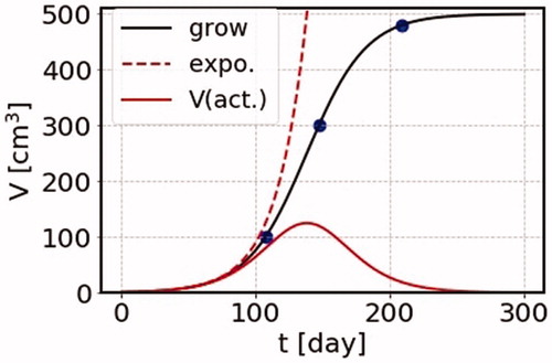
4.2. Active- and inactive-cells

In Figure 1 we show the time dependence of volume growth, together with the one of active cell volume (solid red curve) defined in Equation (10)(10) $$N\left(t\right)=N^{\mathrm{active}}\left(t\right)+N^{\mathrm{inactive}}\left(t\right)\{\begin{array}{c}{N}^{\mathrm{active}}\left(t\right)=N\left(t\right)\left(1-\frac{N\left(t\right)}{N_m}\right), \\ N^{\mathrm{inactive}}\left(t\right)=N\left(t\right)\left(\frac{N\left(t\right)}{N_m}\right). \end{array}$$(10) , together with the behavior of volume growth function itself in unit of day (solid black curve) for the case of the terminal volume $V_m=500{cm}^3;$ the growth function tends to terminal volume $V_m.$ It is noted that the effect of irradiation is proportional to the active cell volume. Later we present the effect of cancer therapy taking three cases where the initial volumes are $V_0=100,\mathrm{ }300\text{ and }480{\mathrm{cm}}^3$ with the same terminal volume $V_m=500{cm}^3,$ where the corresponding initial volumes of cancer treatment are shown by three blue circles for later references.

The formula (10) together with Equation (13)(13) $$\frac{dV\left(t\right)}{dt}=\left(\lambda -b_{1}d\left(t\right)\right)V\left(1-\frac{V\left(t\right)}{V_m}\right),\mathrm{ }$$(13) naturally explains the essence of the phenomenological rule almost exactly, which reminds us of the law of Bergonie and Tribondeau proposed in the old days in 1906 (Bergonié and Tribondeau 2003; Vogin and Foray 2013).

1. X-rays are more effective on cells which have a greater reproductive activity: quickly dividing tumor cells are generally more sensitive than the majority of body cells.

2. The most sensitive cells are those that are undifferentiated, well-nourished, divide quickly and are highly metabolically active.

Indeed, amongst the body cells, the most sensitive are spermatozoa and erythrocytes, epidermal stem cells, gastrointestinal stem cells.

Now, we should add two important comments here.

First, although many oncology lectures cite the law of BT as a founding principle of radio-therapy we should be careful to avoid misleading mixture of the notions of stem cells, proliferation, differentiation along with radio-sensitivity, which is still to be clarified. Indeed, in the review (Vogin and Foray 2013), three kinds of errors are pointed out,

1. Tumors are not, necessarily more radiosensitive than normal tissues.

2. Proliferation rate are not necessarily correlated with cellular death after irradiation

3. Radio-sensitivity and cancer susceptibility after irradiation are two different notions.

Second, we should note that above cell growth property mostly appears in the case of low LET radiation exposure such as X-ray or gamma-ray. They will attack certain parts of DNA sequences or certain loci, which were named as ‘sensitive zones’ in the original target theory. If we consider high LET radiation, for example heavy ion irradiation, the ‘sensitive zone’ in the target theory maybe the entire cell itself independently of the details of the internal structure of a cell. This is just like dropping a bomb on the entire house, instead of just breaking certain sensitive parts of the house. This interesting problem is an issue for further investigation.

4.3. Dose rate dependence

Now we make an interesting remark. If we choose the dose rate, (17) $$d=\frac{\lambda }{b_1}, \left(\lambda -b_{1}d=0\right) \to \frac{dV}{dt}=0,$$(17) the volume is kept constant independently of time. Since the SS model is able to treat any time profile of irradiation, we can calculate a case of continuous irradiation in cancer treatment. We take an example of a tumor with the would-be terminal volume of $V_m=500{cm}^3,$ and perform irradiation continuously for a long time starting at the time of the cancer volume 100 cm³. We take the growth rate $\lambda$=0.045/day and $b_1$=0.045 Gy⁻¹. The results are shown in Figure 2 for cases of the dose per day as 0, 0.2, 0.4, 0.6, 0.8, 1, 1.3, 2, 3 and 5 Gy. 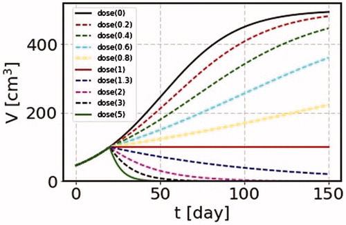For the case where the cancer volume is kept constant with $d$ =1 Gy/day, we can perform other effective treatments. Although such treatment might be unrealistic under the circumstance of the present clinical condition, it is still worthwhile to be tested, or we can confirm the phenomena in some experimental data.

Figure 2. We take the parameters $\lambda$= 0.045/day, the terminal volume $V_m$ = 500 cm³, and $b_1$ = 0.045 Gy⁻¹. We show many cases where irradiation is made continuously for 150 days with the dose per day as 0, 0.2, 0.4, 0.6, 0.8, 1, 1.3, 2, 3 and 5 Gy. For the case of the dose rate corresponding the growth rate, the cancer volume is unchanged as shown by the solid curve (dose(1)).

5. Comparison with experimental data

The LQ model has long been considered as the best-fitting model to describe the survival function, and frequently utilized in the assessment of the radiotherapy treatment planning (Emami et al. 2015; Rühm, Azizova, et al. 2015; Rühm, Woloschak, et al. 2015). The survival function shows sometimes non-linear behaviors in the log plot, which forces scientists to include the quadratic term in the LQ model. Leaving the detailed history to the review by Vogin and Foray (2013), let us quote their final concluding remark: ‘More sophisticated mathematical models are needed to consolidate the change of paradigms’. Further many studies have been performed to improve problems of the LQM treatment in the clinical plan. Especially in the field of radiotherapy, it is remarkable to see various models trying to accommodate the biological radiation effect using the LQ model, which is expressed in terms of the total dose D to the t dependent dynamics due to the proliferation of tumor. These models are the ZM model and related works (Zaider and Minerbo 2000), the clinical model using the proliferation saturation index (PSI) (Rockne et al. 2010; Prokopiou et al. 2015; Tariq et al. 2016; Sunassee et al. 2019), and the clinical model using the biological effective dose (BED) (Fowler 1989, 2010), together with many related works (Tobias 1985; Sottoriva et al. 2010; Borasi 2016; Borasi & Nahum 2016).

The most serious point is how to connect the LQ model with the differential equation to account for the growth effects. They have to assume the instantaneous approximation using the LQ model (Harpold et al. 2007; Prokopiou et al. 2015; Sunassee et al. 2019), or to derive the differentiated LQM form, of which the reaction rate is divided into the time-dependent and time independent parts. Although the latter term can be identified as the growth factor together with an additional constant, which corresponds to $\lambda$ in the SS model, the time dependent term is inevitably left unknown, and had to be replaced with another information of so-called TCP (Millar and Canney 1993; Zaider and Minerbo 2000; Keinj et al. 2011; Watanabe et al 2016; Ponce Bobadilla et al. 2018; Nuraini and Widita 2019). On the other hand, using the integrated expression of the LQ model in the fractionation procedure, the so called BED is adapted in constructing the clinic plan of radiation therapy. It is, however, difficult to take account of the information such as the cell growth process, and the correction term is introduced in their global sum (Fowler 1989, 2010). We shall write all the details of the LQ model and its comparison with the SS model in a separate forthcoming paper.

In this section, by picking up a few examples, we show how the SS Model reproduces experimental data.

5.1. Normal cell in vitro; WI-38

The first example is the experiment on the time dependence of the number of cells in the long-term exposure. As an example, we pick up the data using WI-38 (Shimura et al. 2014), which is a diploid human cell line derived from the lung tissue of a fetus. We show in Figure 3, the calculated results corresponding to their data (Shimura et al. 2014). The time dependence of the number of cells is measured to see the effect of long-term radiation exposure. The parameters $\lambda$ and $V_m$ can be read off from their data without irradiation in Figure 1 of Shimura et al. (2014). In this figure we can see that our model reproduces quite well the experimental data in vitro using the cell WI-38 line. The number of cells increases about 10 times per 7 days, and grows more or less exponentially as the time is increased. Hence we take $V_m=\infty$ and (18) $$\lambda =0.38 {\mathit{day}}^{-1}.$$(18)

Figure 3. The SS model results on the numbers of cells in a WI-38 colony in arbitrary unit as a function of time in day. The irradiation is made twice a day for 6 days with one day break per week. We show the predicted curves with different irradiation time schedule, with irradiation with d = 0.01, 0.05, 0.5, 1 and 2 Gy/fraction (solid lines dose(0.01-2)), together with the corresponding data points (circle dots nearby each solid lines) up to 22 days, where our model is applicable to the experimental data. The parameters used for the calculation are $\mathrm{\lambda }\mathrm{ }$= 0.38 day⁻¹, V_m = 100, and b₁ = 0.0855 Gy⁻¹. This shows that our SS model nicely reproduces the experimental data.

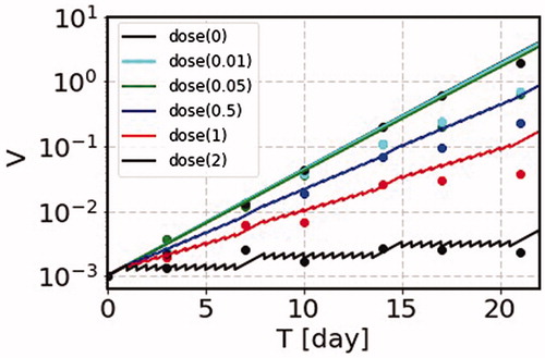
Furthermore, we can read off the case of roughly no change of the number from the data of Figure 1 of Shimura et al. (2014). We take (19) $$b_1=0.0855 {Gy}^{-1},$$(19) which is amazingly close to the value of the mouse data of Equation (5)(5) $$a_0=2.13·{10}^{-8} \left[\frac{1}{\mathrm{hour}}\right], a_1=4.95·{10}^{-4} \left[\frac{1}{Gy}\right],$$(5) .

The fractional irradiation is made twice a day, and the calculation is done with 12 h interval for 6 days a week. The dose rates used for the calculation are d = 0.01, 0.05, 0.5, 1 and 2 Gy/fraction. The numbers of cells as functions of time are shown for these dose rates including the one without irradiation. The experimental data are denoted by dots with various colors from Figure 1 of Shimura et al. (2014). The SS model prediction is consistent with experimental data (Shimura et al. 2014). This tendency can be recognized from the feature of the time dependence of a colony volume calculated with the SS model in Figure 2, where the data points of WI-38 correspond to the curves showing the growing tendencies from the black solid curve until the red solid line.

We can find similar behaviors in the data using cancer cells, such as human U2OS, glioma MO59K cell lines, in vitro. These experimental data are very interesting (Matsushita et al. 1999; Magae et al. 2003, 2011; Mu et al. 2003; Ogata et al. 2005; Nakajima et al. 2007, 2017; Dewan et al. 2009), and we shall analyze them in a forthcoming paper.

5.2. Survival function

The second example is survival functions found in textbook. Examples of survival functions are cell survival curves for four human tumor cell lines shown in Figure 1 of Steel et al. (1989), the dose rate dependence of human cell line (HX118) shown in Figure 2 of Kelland and Steel (1986), and cell survival curves of Chinese Hamster (V79S171) shown in Figures 2 and 4 of Chadwick and Leenhouts (1973). Those examples show the dose rate dependence and the effect due to the cell proliferation. It is very interesting to calculate the survival functions using the SS model, since the S functions are used to determine the coefficients $\mathrm{\alpha }$ and $\mathrm{\beta }$ in the LQ model. In particular, the necessity of the $\mathrm{\beta }$ term is emphasized by the curving behavior in the log plot of the S function.

Figure 4. We show the survival functions for the case of various dose rates; d = 369,121,518 Gy/day with $N_m$ = 1.1 in the left figure (case 1) and $N_m$ =100000 in the right figure (case 2) where we take $N_0$ = 1. The vertical axis is the total dose D instead of time t. We take the growth rate as $\lambda$ = 0.5 day⁻¹ with $b_1$ = 0.2 Gy⁻¹.

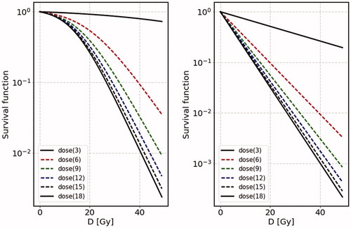
In the SS model the survival function $S\left(D\right)$ is calculated easily for the case of constant dose rate d from Equation (14)(14) $$V\left(t\right)=\frac{V_m{V}_0{e}^{\left(\lambda -b_{1}d\right)t}}{V_m+V_0\left(e^{\left(\lambda -b_{1}d\right)t}-1\right)},\mathrm{ }$$(14) , (20) $$S\left(D\right)=\frac{V\left(D\right)}{V_0}=\frac{V_m\hspace{0.17em}\text{exp}\hspace{0.17em}\left({\alpha }_{SS}D\right)}{V_m+V_0\left(\hspace{0.17em}\text{exp}\hspace{0.17em}\left({\alpha }_{SS}D\right)-1\right)},{\alpha }_{SS}\equiv -b_1+\frac{\lambda }{d},$$(20) where we have expressed $S\left(D\right)$ in terms of the total dose $D=dT$ instead of the total irradiation time T. The above expression says that the parameter $\mathrm{\alpha }$ corresponds to not only $b_1$ but additional term $\mathrm{\lambda }/d,$ which depends on dose rate: for higher dose rate, the contribution of this term becomes lower, but for lower dose rate the slope around threshold (namely around S = 1) becomes flatter and flatter. This can nicely reproduce the characteristic feature of Survival function². We should stress that the above expression makes us to understand the characteristic feature of the S function and indeed naturally explains why the dose rate dependence appears in the S function; it comes from the factor, $\lambda /d$ in Equation (20)(20) $$S\left(D\right)=\frac{V\left(D\right)}{V_0}=\frac{V_m\hspace{0.17em}\text{exp}\hspace{0.17em}\left({\alpha }_{SS}D\right)}{V_m+V_0\left(\hspace{0.17em}\text{exp}\hspace{0.17em}\left({\alpha }_{SS}D\right)-1\right)},{\alpha }_{SS}\equiv -b_1+\frac{\lambda }{d},$$(20) . Additionally, the S function depends on the maximum volume $V_m,$ which controls the amount of active cells in the system.

In Figure 4, we show calculated results on the S function for two cases, where the initial number $N_0$ is close to the terminal number $N_m$ (case 1), and well below the terminal number $N_m$ (case 2). The growth rate for this example is taken to be $\lambda$=0.5 day⁻¹. We take $N_0$=1 for presentation of the S function. We take the coefficient $b_1$=0.2 Gy⁻¹. As for the dose rate, we take d = 369,121,518 Gy/day. In the left figure, we show the results of case 1, where $N_m$=1.1. In this case (left figure) the S functions show bending behaviors for various dose rates. On the other hand, for the case 2 (right figure) the S functions show straight curves with various slopes depending on the dose rates. It turns out that, as for the dose dependence, the higher the dose rate the steeper its slope becomes, with each slope tends to $b_{1}d$ as d becomes larger and larger. Further the behavior around the small D, its slope becomes almost flat for case 1, while it is kept almost linear for case 2. Such features are to be compared with the data of survival function, commonly seen in Figures 1 and 2 of Steel et al. (1989), and Figures 2 and 4 of Chadwick and Leenhouts (1973). The above figures show clear dose rate dependence; around the threshold the higher the dose rate is, the steeper the slope of the S function in the log plot. Sometimes near the threshold, the gradient is almost zero, while the gradient is considerably large and rapidly decreasing in a straight line. In the SS model, the S function plotted in the log scale shows a tendency that the slope becomes even larger as the dose rate increases.

On the contrary to the SS model, the essence of the LQ model is (21) $$S\left(D\right)=\exp \left(-E\left(D\right)\right), E\left(D\right)=\alpha D+\beta D^2,$$(21) with two parameters $\mathrm{\alpha },$ $\mathrm{\beta }.$ These two parameters are used to fit the S functions. $\mathrm{\beta }$ is necessary to express the S function with bending behavior. The S function decreases with total dose D and never increases even if the whole cell system has some repair or increasing power. This time dependent contribution cannot be included so far as $E\left(D\right)$ depends only on the total dose D. Therefore, the above two parameters inevitably have to be changed according to the value of the dose rate. On the contrary, in the SS model the parameter $b_1$ is kept constant, but the S function shows the bending behavior.

5.3. Cancer stages of starting treatment

Now let us see what happens in actual cases for the time dependence of the cancer volume for the cases of the cancer treatment. We here pick up non-small cell lung cancer (NSCLC) (in Figure 2 of their paper), which has been analyzed by the PSI model (Prokopiou et al. 2015). Further comparisons are made in their recent publications (Sunassee et al. 2019). In Figure 1 of the PSI model (Sunassee et al. 2019), two cases are shown with detailed measurements of the volume of cancers using largely different ${\lambda }_p$ and ${\gamma }_D.$ For these patients, the agreements are very good. In Figure 2 of this paper (Sunassee et al. 2019), they show comparisons of the PSI model with the common values of ${\lambda }_p$ and ${\gamma }_D$ by changing slightly the PSI values. The agreements are good. The SS model is able to reproduce the results of the PSI model by taking almost the same parameters. Later we will show our choices of parameters in the SS model for the reproduction of the hospital data.

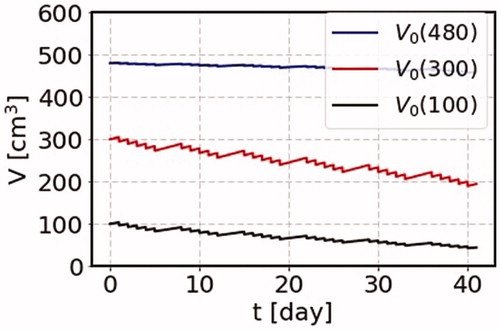
We show first how different results are obtained for the time dependent behavior if we want to know the information beyond the instantaneous approximation such as time duration effects or dose rate dependence and so on. This subsection provides our calculated result of the SS model on the change of cancer volume as a function of time due to the cancer treatment, by demonstrating three cases of different initial volumes, namely for the cases where irradiation starts one day after the cancer volumes are $V_0$= 100, 300, and 480 cm³. These three cases corresponding to the points of the blue circle dots in Figure 1, with the common terminal volume $V_m$= 500 cm³. The parameters we use here is the ones to reproduce the PSI results. (22) $$\lambda =0.045{\mathit{day}}^{-1}, b_1=0.045{Gy}^{-1}.$$(22)

The total dose is 2 Gy in a short period in a day in the SS model with the cancer growth rate $\lambda$=0.045 day⁻¹. The irradiation starts with the initial volumes 100, 300 and 480 cm³, where the terminal volume is 500 cm³. The results are shown in Figure 5. For the case of large initial volume, the effect of the cancer treatment is small. For the intermediate initial volume, the effect of the cancer treatment is large as the number of active cancer cells is large, and almost at the peak of the number of active cells as shown by the red curve in Figure 1. On the other hand, for the smallest initial volume, the cancer treatment is found to work more effectively to reduce the cancer volume.

Figure 5. The change of the cancer volume as a function of time due to the cancer treatment. We use the parameters $b_1$ = 0.045 Gy⁻¹ and the total dose, 2 Gy a day, growth rate $\lambda$ = 0.045 day⁻¹. We consider three cases of the initial volumes for a cancer with the terminal volume of 500 cm³. We start irradiation one day after the cancer volume is 100, 300, and 480 cm³. These three cases are shown by circle dots on the solid curve (grow) in Figure 1.

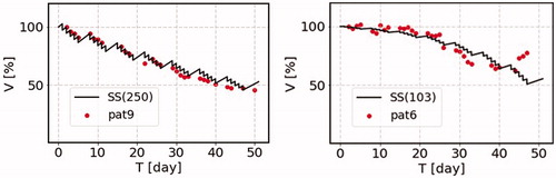
We demonstrate the comparison of the predictions of the change of the cancer volume as a function of time due to the cancer treatment with real hospital data in Figure 6. We here pick up two typical examples of the data of NSCLC patients, where the time dependence of the tumor volume of each patient is available. The one is named as ‘patient 6’ and the other is ‘patient 9’ (Sunassee et al. 2019). The radiation is exposed with the total dose of 2 Gy a day in working days with no irradiation in weekend. The parameters we take are the growth rate λ = 0.045 day⁻¹, which is kept the same for these two cases, and b₁ = 0.045 Gy⁻¹ and V_m = 250% of the initial volume for patient 9 (left figure), and b₁ = 0.085 Gy⁻¹ and V_m = 103% of the initial volume for patient 6 (right figure). The result of the patient 6 is very interesting, since this result is reproduced only by including the b1 term in front of the saturation term.

Figure 6. The comparison of the SS model prediction for the cancer volume as a function of time due to the cancer treatment with the real hospital data. We here pick up two typical examples of the data of non-small cell lung cancer (NSCLC) patients, where the time dependence of the tumor volume of each patient is available, which are shown by points normalized to the initial volume (100%). The one is named as ‘patient 6’ and the other is ‘patient 9’ (Sunassee et al. 2019). The radiation is exposed with the total dose of 2 Gy a day in working days with no irradiation in weekend. The parameters we take are the growth rate λ = 0.045 day⁻¹, which is kept the same for these two cases, and $b_1$ = 0.045 Gy⁻¹ and V_m = 250% of the initial volume for patient 9 (left figure), and $b_1$ = 0.085 Gy⁻¹ and V_m = 103% of the initial volume for patient 6 (right figure).

5.4. Duration of treatment

Let us see how the tumor volume changes in time, if we try to make the duration of the treatment schedule shorter by increasing the amount of dose rate. The terminal volume is taken common as $V_m$= 500 cm³. As examples, let us here consider three cases where the total dose is 2, 2.5 and 4 Gy per day in the SS model. The results are shown in Figure 7.

Figure 7. We use the parameters $b_1$ = 0.045/Gy, and the terminal volume is taken common as 500 cm³. We consider three cases for the total dose as 2, 2.5 and 4 Gy for each day, and the irradiation durations are 6, 4 and 2 weeks, respectively. The effect of the irradiation is larger for the larger total dose, and the final cancer volumes are about 25 cm³ for all the three cases within the corresponding treatment durations.

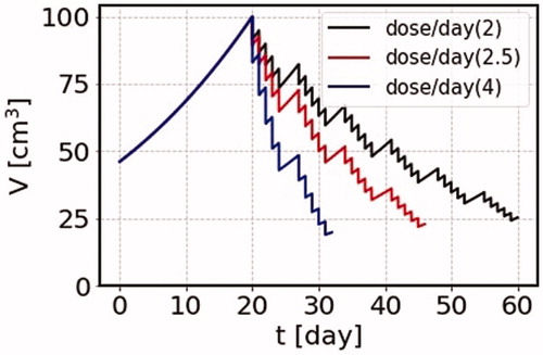
For the case of the total dose of 2 Gy, the volume of the cancer after 6 weeks becomes close to 25 cm³. In order to get the same volume for the four weeks treatment, we can take 2.5 Gy for each day, or for the two weeks treatment, we can take 4 Gy for each day to come up with a similar volume. Of course, the use of larger doses for cancer treatment needs careful assessment of the radiation effects on normal tissues getting irradiated. Although the irradiation effect on normal cells could be also estimated using the SS model by taking account of the fact that the part of tissues, where the cells are active, the effect of irradiation is large, while for the inactive parts of tissues the effect is small. These modern machines and other state-of-the-art techniques are just under development and will make radiation oncologists to significantly reduce side effects while improving the ability to deliver radiation. Nowadays, in the modern technology of the External Beam Radiation Therapy (EBRT), actual areas receiving radiation depends on the feature of cancer and also on the technique of how correctly a position can be spotted for each treatment. Radiation can be delivered specifically to an organ or encompass the surrounding area, including the lymph nodes. For example, three-dimensional conformal radiation therapy (3 D-CRT) can deliver more precisely by using a special technique and may reduce the chance of injury to nearby body structures drastically. Thus, combined with those techniques, radiation oncologists may be able to give higher doses of radiation safely. We expect the collaboration of those techniques with the SS estimation will provide a greater cancer cure program.

6. Discussion

We should emphasize here the meaning of the parameters $a_1$ and $b_1$ from the viewpoint of the target theory. They are the reaction rates of physical stimulus processes caused by radiation exposure. Although we have not yet known the exact structure of the target in cell, in old days they identified it as ‘sensitive zone’, which nowadays might be identified a specific part of DNA sequence. This is why Muller (Muller 1927, 1932) and Russell (Russell 1951, 1963, 1965; Russell et al. 1958; Russell and Kelly 1982a, 1982b) did their animal experiments (Drosophila, Mouse, respectively) using the famous SLT, where they measured the mutation frequencies of specific phenotype visible loci. This determines a reaction rate $a_1$ per locus, which we have already found a remarkable fact that the parameter $a_1$ per locus are almost of the same order in Drosophila and mouse cases (Bando et al. 2019), although there exist 2 or 3 factors difference. This reminds us the comment by Neel, ‘DNA is DNA’. This indicates that the target (sensitive zone) can be identified by a specific locus, a part of DNA sequence, is commonly affected by radiation irrespectively of the species of organism.

Also we have made an interesting remarkable coincidence of the spontaneous mutation frequency found in mouse experiments (Equation (6)(6) $$a_0/b_0\sim {10}^{-5}, a_1/b_1\sim {10}^{-3}\left[1/Gy\right]$$(6) ) with the mammalian genome mutation rate obtained from the biological evolution theory (Kumar and Subramanian 2002) which was found in the evolutional biology.

On the other hand, as for $b_1,$ the value of which we got is almost 10³ times larger than $a_1$ from the mouse data, as is noted in section 2, Equation (5)(5) $$a_0=2.13·{10}^{-8} \left[\frac{1}{\mathrm{hour}}\right], a_1=4.95·{10}^{-4} \left[\frac{1}{Gy}\right],$$(5) . We have found that this reaction rate indicates the so-called reaction rate yielding cell death (Bando et al. 2019). Such cell death caused by radiation may be almost commonly induced independently of any cell and we may assume that the cell death rate does not depend on even cell types, irrespectively of normal, mutated or cancer cell, and even bacteria. Perhaps this was what Marie Curie had examined, including experiments on bacterial sterilization based on the target theory. At this moment, however, this is only our speculation, but we have here found that it can be confirmed to study the case of radiation cancer treatment. It is really interesting to see whether we may be led to a unified understanding of the biological effects caused by radiation exposure and the parameters can be determined independently of the species of the organism.

7. Conclusion

We extended the WAM model to construct the SS model for the use of cancer therapy, which beautifully explains the old Bergonie and Tribondeau law by introducing the concept of active and inactive cells. The SS therapy equation coincides with the one presented in the PSI model of Prokopiu et al. only for the case of short irradiation treatment, where the equation of the SS model coincides with those of the PSI model for the case of instantaneous irradiation. However, the SS therapy equation is expressed in a differential form and can be used in any situation, not only for a short fractional irradiation case but also for a continuous irradiation case. If we take the same parameters as those of the hospital data, we can reproduce all the patient data as demonstrated by previous studies. We discussed the case where the dose rate is increased for a shorter treatment time. We also showed the case where we make continuous irradiation on cancer.

We made comparisons of the SS model predictions with various experimental data. We took the numbers of cells in a WI-38 colony for various dose rates as a function of time (Shimura et al. 2014). The experimental data corresponded the growing part of the cancer volume in the continuous irradiation curve shown in Figure 2. The calculated results compared well with the experiment. We took then the experimental data on the survival functions in vitro, which have been obtained for many cases. They showed two characteristic behaviors. One is the case (case 1), where the S functions bent down in the log plot as a function of the total dose, and the other is the case (case 2), where the S functions dropped down straight in the log plot. We made calculations using the SS model and showed that the bending behavior in case 1 was obtained when the maximum volume $V_m$ was slightly above the initial volume, while the straight behavior in case 2 was obtained when the maximum volume was much larger than the initial volume. The SS model was able to produce bending curves in the S function, which was reproduced by the $\mathrm{\beta }$ term in the LQ model.

We hope that our findings will open the door of unified understanding of across species dynamics of cell biology.

Acknowledgements

We are grateful for many fruitful discussions with Prof. Maki for ultra-fast and frequent damage-repair process of cells in biological body, and Prof. Teshima on radiation treatment of cancer in hospital. We appreciate the efforts of Prof. Magae to provide us with many illuminating information on biological experiments. We thank Prof. Wada for responding our request to find M. Curie's paper in the library of his university.

Disclosure statement

No potential conflict of interest was reported by the author(s).

Additional information

Funding

This research is supported by KAKENHI Grant in-Aid for Scientific Research (B) [16H04637, 16H03094] and for Challenging Exploratory Research [15K14291, 15K12204].

Notes on contributors

Masako Bando

Masako Bando, PhD, is a Researcher of Research Center for Nuclear Physics, Osaka University and Yukawa Institute, Kyoto University. Her specialty is physics (elementary particle theory), and she extended her research to traffic flow theory, economic physics and now to to radiation biology. She is extending the radiation protection problem to radiation therapy. Further she is now eager to get the essence of evolution theory by understanding them microscopic view point.

Yuichi Tsunoyama

Yuichi Tsunoyama, PhD, is an Assistant Professor and a radiation protection supervisor of Radioisotope Research Center, Agency for Health, Safety and Environment, Kyoto University. His research field is radiation biology, and his interest is biological effects of radiation at the molecular and cellular level.

Kazuyo Suzuki

Kazuyo Suzuki, MD, PhD, is Program-Specific Assistant Professor of Preemptive Medicine and Lifestyle-Related Disease Research Center, Kyoto University. Her research interests lie in nutrition science, metabolism, and preventive medicine.

Hiroshi Toki

Hiroshi Toki, is a PhD, of Osaka University in 1974. He is an Emeritus Professor of Research Center for Nuclear Physics, Osaka University. His research field is theoretical Nuclear Physics, Electric circuit, and the biological effect of radiation.

Notes

1 We plan to place the SS cancer therapy simulator on the WEB.

2 Such characteristic features are investigated from different point of view by Chadwick and Leenhouts (1973).

References

- Bando M, Kinugawa T, Manabe Y, Masugi M, Nakajima H, Suzuki K, Tsunoyama Y, Wada T, Toki H. 2019. Study of mutation from DNA to biological evolution. Int J Radiat Biol. 95(10):1390–1403.
- Bando M, Manabe Y, Wada T. 2017. From DDREF to EDR–What the history of LNT indicates. Paper presented at 2017 ERPW Conference in Paris; France; 9–13.
- Bergonié J, Tribondeau L. 2003. Interpretation of some results from radiotherapy and an attempt to determine a rational treatment technique. Yale J Biol Med. 76(4–6):181–182. translated from Interprétation de quelques résultats de la radiothérapie et essai de fixation d’une technique rationnelle. Comptes rendus hebdomadaires de l’Académie des sciences (1906) 983–985.
- Bodgi L, Canet A, Pujo-Menjouet L, Lesne A, Victor JM, Foray N. 2016. Mathematical models of radiation action on living cells: From the target theory to the modern approaches. A historical and critical review. J Theor Biol. 394:93–101.
- Borasi G. 2016. Comment on ‘Predicting the efficacy of radiotherapy in individual glioblastoma patients in vivo: a mathematical modeling approach'. Phys Med Biol. 61(7):2967.
- Borasi G, Nahum A. 2016. Modelling the radiotherapy effect in the reaction-diffusion equation. Phys Med. 32(9):1175–1179.
- Chadwick KH, Leenhouts HP. 1973. A molecular theory of cell survival. Phys Med Biol. 18(1):78–87.
- Curie M. 1929. Sur l’étude des courbes de probabilité relatives à l’action des rayons X sur les bacilles. Comptes Rendus L’Académie Des Sci. 188:202–204.
- Dewan MZ, Galloway AE, Kawashima N, Dewyngaert JK, Babb JS, Formenti SC, Demaria S. 2009. Fractionated but not single-dose radiotherapy induces an immune-mediated abscopal effect when combined with anti-CTLA-4 antibody. Clin Cancer Res. 15(17):5379–5388.
- Dhawan A, Kohandel M, Hill R, Sivaloganathan S. 2014. Tumour control probability in cancer stem cells hypothesis. PLoS One. 9(5):e96093.
- Elkind MM, Whitmore GF, Alescio T. 1964. Actinomycin D: Suppression of recovery in X-irradiated mammalian cells. Science. 143(3613):1454–1457.
- Emami B, Woloschak G, Small W. Jr. 2015. Beyond the linear quadratic model: intraoperative radiotherapy and normal tissue tolerance. Transl Cancer Res. 4(2):140–147.
- Fowler JF. 1989. The linear-quadratic formula and progress in fractionated radiotherapy. Br J Radiol. 62(740):679–694.
- Fowler JF. 2010. 21 years of biologically effective dose. Br J Radiol. 83(991):554–568.
- Galluzzi L, Vitale I, Aaronson SA, Abrams JM, Adam D, Agostinis P, Alnemri ES, Altucci L, Amelio I, Andrews DW, et al. 2018. Molecular mechanisms of cell death: recommendations of the nomenclature committee on cell Death 2018. Cell Death Differ. 25(3):486–541.
- Hanahan D, Weinberg RA. 2011. Hallmarks of cancer: the next generation. Cell. 144(5):646–674.
- Harpold HLP, Alvord EC Jr, Swanson KR. 2007. The evolution of mathematical modeling of glioma proliferation and invasion. J Neuropathol Exp Neurol. 66(1):1–9.
- Keinj R, Bastogne T, Vallois P. 2011. Multinomial model-based formulations of TCP and NTCP for radiotherapy treatment planning. J Theor Biol. 279(1):55–62.
- Kelland LR, Steel GG. 1986. Dose-rate effects in the radiation response of four human tumour xenografts. Radiother Oncol. 7(3):259–268.
- Kühleitner M, Brunner N, Nowak WG, Renner-Martin K, Scheicher K. 2019. Best fitting tumor growth models of the von Bertalanffy-PütterType. BMC Cancer. 19(1):683.
- Kumar S, Subramanian S. 2002. Mutation rates in mammalian genomes. Proc Natl Acad Sci USA. 99(2):803–808.
- Lea DE. 1946. The inactivation of viruses by radiations. Br J Radiol. 19:205–212.
- Magae J, Furukawa C, Ogata H. 2011. Dose-rate effect on proliferation suppression in human cell lines continuously exposed to γ rays. Radiat Res. 176(4):447–458.
- Magae J, Hoshi Y, Furukawa C, Kawakami Y, Ogata H. 2003. Quantitative analysis of biological responses to ionizing radiation, including dose, irradiation time, and dose rate. Radiat Res. 160(5):543–548.
- Manabe Y, Bando M. 2013. Comparison of data on mutation frequencies of mice caused by radiation with low dose model. J Phys Soc Jpn. 82(9):094004.
- Manabe Y, Ichikawa K, Bando M. 2012. A mathematical model for estimating biological damage caused by radiation. J Phys Soc Jpn. 81(10):104004.
- Manabe Y, Wada T, Tsunoyama Y, Nakajima H, Nakamura I, Bando M. 2015. Whack-a-mole model: towards a unified description of biological effects caused by radiation exposure. J Phys Soc Jpn. 84(4):044002.
- Matsushita S, Nitanda T, Furukawa T, Sumizawa T, Tani A, Nishimoto K, Akiba S, Miyadera K, Fukushima M, Yamada Y, et al. 1999. The effect of a thymidine phosphorylase inhibitor on angiogenesis and apoptosis in tumors. Cancer Res. 59(8):1911–1916.
- Millar WT, Canney PA. 1993. Derivation and application of equations describing the effects of fractionated protracted irradiation, based on multiple and incomplete repair processes. Part I. Derivation of equations. Int J Radiat Biol. 64(3):275–291.
- Mu X, Löfroth PO, Karlsson M, Zackrisson B. 2003. The effect of fraction time in intensity modulated radiotherapy: theoretical and experimental evaluation of an optimisation problem. Radiother Oncol. 68(2):181–187.
- Muller HJ. 1927. Artificial transmutation of the gene. Science. 66(1699):84–87.
- Muller HJ. 1932. Further studies on the nature and causes of gene mutations. Proceedings of the 6th International Congress of Genetics; Ithaca, New York 1: 213–255.
- Naderi S, Hunton IC, Wang JY. 2002. Radiation dose-dependent maintenance of G(2) arrest requires retinoblastoma protein. Cell Cycle. 1(3):193–200.
- Nakajima H, Furukawa C, Chang YC, Ogata H, Magae J. 2017. Delayed growth suppression and radioresistance induced by long-term continuous gamma irradiation. Radiat Res. 188(2):181–190.
- Nakajima H, Mizuta N, Sakaguchi K, Fujiwara I, Mizuta M, Furukawa C, Chang YC, Magae J. 2007. Aberrant expression of Fra-1 in estrogen receptor-negative breast cancers and suppression of their propagation in vivo by ascochlorin, an antibiotic that inhibits cellular activator protein-1 activity. J Antibiot (Tokyo). 60(11):682–689.
- Nakamura I, Manabe Y, Bando M. 2014. Reaction rate theory of radiation exposure and scaling hypothesis in mutation frequency. J Phys Soc Jpn. 83(11):114003.
- Nuraini R, Widita R. 2019. Tumor control probability (TCP) and normal tissue complication probability (NTCP) with consideration of cell biological effect. J Phys Conf Ser. 1245:012092.
- O’Rourke SFC, McAneney H, Hillen T. 2009. Linear quadratic and tumour control probability modelling in external beam radiotherapy. J Math Biol. 58(4–5):799–817.
- Ogata H, Furukawa C, Kawakami Y, Magae J. 2005. A quantitative model for the evaluation of dose rates effects following exposure to low-dose gamma-radiation. Radioprotection. 40(2):191–202.
- Ponce Bobadilla AV, Maini PK, Byrne H. 2018. A stochastic model for tumour control probability that accounts for repair from sublethal damage. Math Med Biol. 35(2):181–202.
- Prokopiou S, Moros EG, Poleszczuk J, Caudell J, Torres-Roca JF, Latifi K, Lee JK, Myerson R, Harrison LB, Enderling H. 2015. A proliferation saturation index to predict radiation response and personalize radiotherapy fractionation. Radiat Oncol. 10(1):159.
- Rockne R, Rockhill JK, Mrugala M, Spence AM, Kalet I, Hendrickson K, Lai A, Cloughesy T, Alvord EC, Jr, Swanson KR. 2010. Predicting the efficacy of radiotherapy in individual glioblastoma patients in vivo: a mathematical modeling approach. Phys Med Biol. 55(12):3271–3285.
- Rühm W, Azizova TV, Bouffler SD, Little MP, Shore RE, Walsh L, Woloschak GE. 2015. Dose-rate effects in radiation biology and radiation protection. Ann Icrp. 45(1_suppl):262–279.
- Rühm W, Woloschak GE, Shore RE, Azizova TV, Grosche B, Niwa O, Akiba S, Ono T, Suzuki K, Iwasaki T, et al. 2015. Dose and dose-rate effects of ionizing radiation: a discussion in the light of radiological protection. Radiat Environ Biophys. 54(4):379–401.
- Russell WL. 1951. X-ray-induced mutations in mice. Cold Spring Harb Symp Quant Biol. 16:327–336.
- Russell WL. 1963. The effect of radiation dose rate and fractionation on mutation mice. In: Sobels FH, editor. Repair from genetic radiation damage. Oxford: Pergamon Press; p. 205–217, 231–235.
- Russell WL. 1965. Studies in mammalian radiation genetics. Nucleonics. 23(1):53–56, 62.
- Russell WL, Kelly EM. 1982a. Specific-locus mutation frequencies in mouse stem-cell spermatogonia at very low radiation dose rates. Proc Natl Acad Sci U S A. 79(2):539–541.
- Russell WL, Kelly EM. 1982b. Mutation frequencies in male mice and the estimation of genetic hazards of radiation in men. Proc Natl Acad Sci U S A. 79(2):542–544.
- Russell WL, Russell LB, Kelly EM. 1958. Radiation dose rate and mutation frequency. Science. 128(3338):1546–1550.
- Sachs RK, Hlatky LR, Hahnfeldt P. 2001. Simple ODE models of tumor growth and anti-angiogenic or radiation treatment. Mathematic Comput Model. 33(12–13):1297–1305.
- Shimura T, Hamada N, Sasatani M, Kamiya K, Kunugita N. 2014. Nuclear accumulation of cyclin D1 following long-term fractionated exposures to low-dose ionizing radiation in normal human diploid cells. Cell Cycle. 13(8):1248–1255.
- Shuryak I, Carlson DJ, Brown JM, Brenner DJ. 2015. High-dose and fractionation effects in stereotactic radiation therapy: analysis of tumor control data from 2965 patients. Radiother Oncol. 115(3):327–334.
- Sobels FH. 1963. Repair and differential radiosensitivity in developing germ cells of Drosophila males. In: Sobels FH, editor. Repair from genetic radiation damage. Oxford: Pergamon Press; p. 179–197.
- Sottoriva A, Verhoeff JJC, Borovski T, McWeeney SK, Naumov L, Medema JP, Sloot PMA, Vermeulen L. 2010. Cancer stem cell tumor model reveals invasive morphology and increased phenotypical heterogeneity. Cancer Res. 70(1):46–56.
- Steel GG, McMillan TJ, Peacock JH. 1989. The 5Rs of radio-biology. Int J Radiat Biol. 56(6):1045–1048.
- Sunassee ED, Tan D, Ji N, Brady R, Moros EG, Caudell JJ, Yartsev S, Enderling H. 2019. Proliferation saturation index in an adaptive Bayesian approach to predict patient-specific radiotherapy responses. Int J Radiat Biol. 95(10):1421–1426.
- Tariq I, Chen T, Kirkby NF, Jena R. 2016. Modelling and Bayesian adaptive prediction of individual patients' tumour volume change during radiotherapy. Phys Med Biol. 61(5):2145–2161.
- Tobias CA. 1985. The repair-misrepair model in radiobiology: comparison to other models. Radiat Res Suppl. 8:S77–S95.
- Tsunoyama Y, Suzuki K, Masugi-Tokita M, Nakajima H, Manabe Y, Wada T, Bando M. 2019. Verification of a dose rate-responsive dynamic equilibrium model on radiation-induced mutation frequencies in mice. Int J Radiat Biol. 95(10):1414–1420.
- van Leeuwen CM, Oei AL, Crezee J, Bel A, Franken NAP, Stalpers LJA, Kok HP. 2018. The alfa and beta of tumours: a review of parameters of the linear-quadratic model, derived from clinical radiotherapy studies. Radiat Oncol. 13(1):96.
- Vogin G, Foray N. 2013. The law of Bergonié and Tribondeau: a nice formula for a first approximation. Int J Radiat Biol. 89(1):2–8.
- Wada T, Manabe Y, Nakamura I, Tsunoyama Y, Nakajima H, Bando M. 2016. Dose and dose-rate dependence of mutation frequency under long-term exposure - a new look at DDREF from WAM model. J Nucl Sci Technol. 53(11):1824–1830.
- Watanabe Y, Dahlman EL, Leder KZ, Hui SK. 2016. A mathematical model of tumor growth and its response to single irradiation. Theor Biol Med Model. 13:6.
- Zaider M, Minerbo GN. 2000. Tumour control probability: a formulation applicable to any temporal protocol of dose delivery. Phys Med Biol. 45(2):279–293.