Reduction of nitrogen pollution in agriculture through nitrogen surplus quotas: an analysis of individual marginal abatement cost and different quota allocation schemes using an agent-based model

Abstract

Nitrogen (N) pollution has mostly been controlled using command-and-control instruments. However, nitrogen surplus permits (NSPs), which are tradeable, can be more cost-efficient in addressing the problem. To model this instrument, we calculated the individual marginal abatement cost curve for a sample of about 3,400 Swiss farms using farm-optimization models implemented in the agent-based agricultural sector model SWISSland. We also used SWISSland to analyze the effects of two NSP distribution systems (grandfathering and land-based allocation) on different farm types. The results showed that different farm types range in their abatement costs to reduce N surplus from an average of −0.04 CHF kg⁻¹ N on arable farms to 51.06 CHF kg⁻¹ N on special crop farms. We also found that N surpluses hardly explain the level of abatement costs. The biggest differences in effects of the distribution scheme were found in intensive livestock farm types such as pig or poultry farms.

Keywords:

• N surplus
• permit
• marginal abatement cost (MAC)
• agent-based modeling
• Switzerland

1. Introduction

Reactive nitrogen (N_r) is a key limiting component in agricultural production. Therefore, N_r from fertilizer and concentrate feeds is used to increase production. However, the benefits of N inputs in agriculture have to be balanced against the environmental damage at both a global and a local scale (Sutton et al. 2011).

In the 1990s, many European countries introduced policies to reduce N pollution in agriculture (Van Grinsven et al. 2013). In Switzerland, the agri-environmental goals defined in 2008 have not yet been achieved (BAFU [Bundesamt für Umwelt], and BLW [Bundesamt für Landwirtschaft] 2016). N surpluses have remained at the high level of 108 kg N per hectare since the 1990s (Spiess 2011). The current Swiss agricultural policies addressing N pollution include cross compliance requiring farms to limit animal stocking density and application following a nutrient management plan and offer regional voluntary programmes for nitrate vulnerable zones (Jan, Calabrese, and Lips 2017). New policy instruments are still needed to reduce emissions further.

Many instruments applied in both Switzerland and other European countries have been command-and-control instruments. These are theoretically less cost-efficient than market-based instruments because the latter allow for flexibility and consider the variability of marginal abatement costs (MAC) (Stuhlmacher et al. 2019; Feess and Seeliger 2013). Research on taxes to reduce N inputs has shown that the demand elasticities for purchasing fertilizer and feed are low (between −0.03 and −0.5) (Berntsen et al. 2003; Finger 2012; Jayet and Petsakos 2013; Mérel et al. 2014; Schmidt et al. 2017).

We therefore wanted to assess the cost efficiency of the new instrument of N surplus permits (NSPs). NSPs are tradeable rights for every kg of N surplus. N surpluses represent the potential environmental damage better than N inputs as they consider N loss in different chemical forms (Oenema, Kros, and de Vries 2003; Stevens and Quinton 2009). Hence, NSPs can be more effective in reducing N pollution than fertilizer taxes. In addition, permits (or quota or rights) allow governments to set a target value for N surplus reduction by limiting the number of permits distributed to the sector (Feess and Seeliger 2013).

NSPs can be auctioned or given freely to farmers. Free distribution can be based on their previous farm practice or their area. Distribution based on previous farm practices (grandfathering) has the advantage of not drastically changing the sector and thus reducing transaction costs (Van der Straeten et al. 2011), whereas distribution based on area has the advantage that farms which already have a low N surplus are not forced to reduce it further. Grandfathering is often criticized, as heavy polluters might profit from the trade, whereas low emitters do not have options for low cost abatement (Woerdman, Arcuri, and Clò 2008; Verde et al. 2019; Clò 2011). Although comparisons between distribution schemes have been carried out for CO₂ (Rosendahl and Storrøsten 2011; Álvarez and André 2015), such an analysis is still lacking for N surpluses.

While there have been assessments of manure shipment, which is a sort of concentration permit trade (Van der Straeten et al. 2011), there have been no assessments of the effects of NSPs on N surplus reduction. No studies to date show the extent to which different schemes for allocating NSPs to farms influence the agricultural sector.

To simulate the trade between the agents, we estimated the marginal abatement cost curves (MACCs) of the individual agents. The different approaches to estimating MACCs include bottom-up approaches (e.g. Hasler et al. 2019; Eory et al. 2018) focusing on a technology portfolio, top-down approaches considering price feedback and focusing on opportunity costs (e.g. Golub et al. 2009) and a mixed approach assessing the interaction of different options under a given pollution ceiling (e.g. Lengers, Britz, and Holm-Müller 2014).

Most studies have focused on greenhouse gas abatement in agriculture; a few exceptions look at N pollution. Ramilan et al. (2011) found that extensive farms have higher MACCs for nitrate discharge than intensive farms. Mack and Huber (2017) noted that N abatement costs are influenced by achieving the optimal level of N input in feeding and fertilization.

This paper aims to extend current knowledge about the effects of NSPs in two dimensions: 1) to analyze how different farm types differ in their N surplus MACs and to discuss the implications of these differences for the design of NSPs based on the heterogeneous farm sample of the Swiss Farm Accountancy Data Network (FADN); 2) to show the effects of two NSP distribution systems on average farm income, average farm size, exit rate, N surplus and NSP selling or buying for different farm types. We analyzed the grandfathering scheme, which distributes NSPs based on previous N surplus, and an area-based distribution scheme, which allocates certificates based on the agricultural area of a farm, and compared these schemes with a scenario where no trade was allowed, which refers to a command-and-control instrument.

We calculated the individual marginal abatement cost curves for the Swiss FADN farms using farm-optimization models implemented in the agent-based agricultural sector model SWISSland (Möhring et al. 2016). We also used SWISSland to analyze the effects of two NSP distribution scenarios: grandfathering and land-based allocation.

2. Methodology

2.1. Overview of the methodological approach

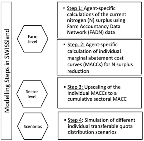
We assessed the effects of NSPs on N surplus reduction for Swiss agriculture using a stepwise approach (Figure 1). Step 1 comprised the calculation of the current farm gate N surpluses for the individual farm agents implemented in the agent-based sector model SWISSland for the year 2015 (see Section 2.3). Step 2 comprised the calculation of MACCs for the individual farm agents using the single farm optimization models of SWISSland (see Section 2.4). Step 3 comprised the calculation of a cumulative MACC for the total Swiss agricultural sector by upscaling the individual MACCs of the FADN farm sample to the total sectoral level using an upscaling tool implemented in SWISSland (Zimmermann et al. 2015) (see Section 2.5). In step 4, the different NSP allocation scenarios were simulated with SWISSland. In this step, SWISSland’s agent-based approach was used to model an NSP trade among farm agents (see Section 2.6).

Figure 1. Overview of the four steps in the modeling procedure to simulate different distribution scenarios for individual transferable quota.

2.2. Overview of the SWISSland model and database

SWISSland is an agent-based agricultural sector model that simulates production and land-leasing decisions for a heterogeneous agent population of 3,400 Swiss FADN farms (Möhring et al. 2016). The farm agents are representative of the Swiss agricultural sector in terms of farm types (6% arable farms, 25% specialized and 4% combined dairy farms, 8% specialized and 3% combined suckler cow farms, 10% horse, sheep and goat farms, 3% specialized and 9% combined pig and poultry farms, 8% vegetable farms, orchards and wineries), agricultural production regions (44% farms in the valley region, 14% in the hill region and 42% in the mountain region) and percentage of organic farms (13.5% organic) (Hoop and Schmid 2013).

For each of the 3,400 farm agents, SWISSland estimates individual land-use and livestock decisions based on a recursive-dynamic farm-level optimization model using positive mathematical programming (PMP) over a period of 11 years. Farm records from the FADN database (three-year averages for the years 2011–2013, further referred to as the base year) were used to calibrate the model and to define the technical coefficients of the optimization models (e.g. production resources, animal- and crop-related yields, costs, prices and direct payments). The agents maximized their farm incomes considering different constraints (Equation (1)(1) $$\mathit{Max}\left({\mathit{Z}}_{\mathit{i},\mathit{t}}\right)\mathit{}=\sum {\mathit{p}}_{\mathit{i},\mathit{t}}{\mathit{x}}_{\mathit{i},\mathit{t}}\mathit{}+\mathit{}{\mathit{d}}_{\mathit{i},\mathit{t}}{\mathit{x}}_{\mathit{i},\mathit{t}}\mathit{}-\mathit{}\frac{1}{\mathit{2}}{\mathit{x}}_{\mathit{i},\mathit{t}}{\mathit{Q}}_{\mathit{i}\mathit{i}}\mathit{}{\mathit{x}}_{\mathit{i},\mathit{t}}$$(1) ). (1) $$\mathit{Max}\left({\mathit{Z}}_{\mathit{i},\mathit{t}}\right)\mathit{}=\sum {\mathit{p}}_{\mathit{i},\mathit{t}}{\mathit{x}}_{\mathit{i},\mathit{t}}\mathit{}+\mathit{}{\mathit{d}}_{\mathit{i},\mathit{t}}{\mathit{x}}_{\mathit{i},\mathit{t}}\mathit{}-\mathit{}\frac{1}{\mathit{2}}{\mathit{x}}_{\mathit{i},\mathit{t}}{\mathit{Q}}_{\mathit{i}\mathit{i}}\mathit{}{\mathit{x}}_{\mathit{i},\mathit{t}}$$(1) $$\mathrm{subject\; to}:\mathit{}{\mathit{A}}_{\mathit{w,i}}{\mathit{x}}_{\mathit{i}}\mathit{}\le \mathit{}{\mathit{B}}_{\mathit{w}}\text{and}{\mathit{x}}_{\mathit{i}}\mathit{}\ge 0$$

The farm income Z_i,t was calculated by adding direct payments (d_i,t) and market revenues from farm activities i (p_i,t: price; x_i,t: production quantities) and subtracting the quadratic cost term (Q_ii: symmetric and positive [semi-definitive] matrix; see Equation (2)(2) $${\mathit{Q}}_{\mathit{ii}}=\mathit{}\frac{1}{{\mathit{\rho }}_{\mathit{i}}}\mathit{*}\mathit{}\frac{{\mathit{\pi }}_{{\mathit{i},\mathit{t}}_0}}{{\mathit{x}}_{{\mathit{i},\mathit{t}}_0}}$$(2) ). (2) $${\mathit{Q}}_{\mathit{ii}}=\mathit{}\frac{1}{{\mathit{\rho }}_{\mathit{i}}}\mathit{*}\mathit{}\frac{{\mathit{\pi }}_{{\mathit{i},\mathit{t}}_0}}{{\mathit{x}}_{{\mathit{i},\mathit{t}}_0}}$$(2) where $x_{{i,t}_0}$ represented the observed production levels and ${\pi }_{{i,t}_0}\text{the revenues}$ in the base year t_0. ρ_iwas the supply elasticity which was considered as 1.

The individual farm models were optimized based on the constraints of available quantities B of the resource endowment w that was not permitted to be exceeded by the demand A for the quantity x_i of resource endowment w. Examples of limited resources are animal housing capacities, land endowment and family labor resources. The cross-compliance measure “Suisse-balance” restricts the application of fertilizers to 110% of the crop needs (Schmidt et al. 2017). If this limit is exceeded, farmyard manure must be exported to other farms (Jan, Calabrese, and Lips 2017).

SWISSland models farm exit or farm succession decisions based on income criteria when the manager of a farm agent reached pension age. If farming activities were given up, the agent’s area was leased to a neighboring farm agent. The agents’ share of off-farm work observed in the FADN data in the base year remains unchanged over the whole modeling period. An ‘overview design concepts and details’ (ODD) protocol of the model is provided by Zimmermann et al. (2015).

2.3. Calculation of the current farm gate N surpluses for the individual heterogeneous farm agents

To assess the individual farm agents’ N surpluses, a farm gate N balance was introduced into the single farm optimization models. This balance accounted for all N inputs entering the farm via fertilizers, feeds, purchased animals, and deposition and fixation by legumes, and subtracted the N leaving the farm via sold animal and plant products (Schmidt et al. 2017). Unlike soil surface N balances, farm gate N balances do not consider farm internal N fluxes such as feed produced on the farm or farmyard manure applied to the fields (Oenema, Kros, and de Vries 2003) (see Figure 2). Farm gate N balances are supplementary to nutrient management plans because they also account for importation of feeds (Pellerin et al. 2017).

Figure 2. The model calculates for every agent a farm gate nitrogen (N) balance to estimate the N surplus. The agent can reduce the N surplus by the reduction of inputs or by changing the production to products with higher N use efficiencies.

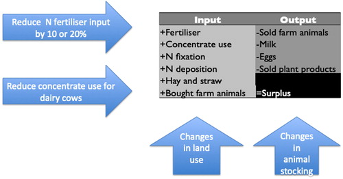
The FADN farms’ N inputs through fertilizers were estimated based on their total fertilizer costs and divided by the nutrient prices, taking into account recommended fertilizer application ratios (Agridea 2013a). Similarly, concentrate inputs for animal production activities were estimated and distributed using typical feed mixtures and their N contents (Agridea 2013b). Average values were chosen for N deposition (19 kg ha⁻¹) (Jan, Calabrese, and Lips 2013). For N fixation, the standard values for different legumes and grassland types were applied (Boller, Lüscher, and Zanetti 2003). For living animals, carcasses and plant products, values per kilogramme were used (Flisch et al. 2009). This approach led to an underestimation of the sectoral N surplus of Swiss agriculture by 8% (Schmidt et al. 2017). We corrected for this difference by adjusting the upscaling factor to meet the published sectoral N surplus in the base year.

2.4. Calculation of individual marginal abatement cost curves

We estimated each agent’s MACC for year 2 after the base year by calculating the difference in farm income with a restricted and an unrestricted farm gate N balance. The second year of the simulation was chosen because Swiss agricultural policy underwent significant changes in 2014 (Mann and Lanz 2013). The MACC was only estimated for farms with positive N surpluses, because farms with negative N surpluses should not further reduce N surpluses due to soil depletion. Consequently, 3.6% of the farms were excluded; the majority consisted of special crop farms (12.3%), arable farms (9.4%) and combined suckler cow farms (9.4%).

In a first run, the N surplus of every agent was calculated without implementing the new N surplus restriction. However, the agents needed to fulfill the current nutrient management plan. The estimated N surplus without restriction was reduced in 10% steps down to −70% of the initial level. For each step, the difference in farm income was divided by the reduced amount of N surplus to calculate the marginal abatement costs of the step. We assumed constant prices because the import quotas might adapt to the new production quantity. The amount of shipped farmyard manure was disregarded because we assumed that agents accepting farmyard manure under current conditions would demand higher prices to accept additional manure if they had a limit, and thus the costs remained on the farms with too high nutrient balances, increasing their MACC.

We considered four different N abatement options in the farm optimization models:

1. Reduction of N fertilization inputs by up to 20% in field crop activities such as wheat, barley, rape seed, sunflower seed, sugar beets, maize and potatoes. For this, yield functions were estimated with a quadratic function as suggested by Busenkell (2004) by relying on the FADN data. The estimated parameters of the yield function are presented in Table A.2 in the appendix (online supplemental data).

2. Reduction of concentrate feeds in milk production (explained in detail in Mack and Huber 2017).

3. Land-use change toward less intensive production activities for which additional ecological direct payments are provided.

4. Reduction in animal stocking density.

All these abatement options affect the variable costs, the production volumes and the associated N outputs. A sensitivity analysis for the model response in N surplus has been reported in Schmidt et al. (2017). We calculated the average abatement costs for each farm type classified by Meier (2000) (see Table A.1 in the appendix [online supplemental data]).

2.5. Upscaling the individual MACCs to a cumulative marginal abatement cost curve

The cumulative MACC aggregates the individual MACCs. For this curve, we first upscaled the N surplus of every agent based on the upscaling factors of SWISSland (Zimmermann et al. 2015). Then we aggregated the marginal costs by integrating the amount of N surplus reduction at a given level for 1 to 300 CHF (1 CHF ≈ 1 USD) in steps of 1 CHF.

2.6. Individual transferable quota distribution scenarios

We tested: 1) a “Grandfathering” scheme where every agent received certificates based on 80% of its previous N surplus. If land was traded in this scenario, the new owner of the land received 80% of the average N surplus of all Swiss farms; 2) an “Area-based” scenario where the distribution of NSPs was based on agricultural area. Every agent received a permit for 88 kg N surplus per hectare, roughly equivalent to 80% of the current average N surplus per hectare in Switzerland; and 3) a “No trade” scenario, where every agent needed to reduce the N surplus by 20%, which refers to a command-and-control scenario. Newly leased land received the same amount of NSPs as already attained land. Based on the cumulative MACC, we derived the price of the NSP for a cumulative reduction of 20% of the N surplus. The level of 20% was selected to compare the results with an N levy presented in Schmidt et al. (2017). For every agent, the program checked how much to reduce for this price and if they needed to buy additional NSPs or were able to sell some. We tracked the agent’s behavior in terms of adaptation strategies to the scenarios, such as exiting from farming, leasing land, buying additional NSPs or selling NSPs to other farmers, in combination with a reduction of the agent’s N surplus.

3. Results

3.1. Abatement costs for each farm type

The variation in MACs between the SWISSland agents on every reduction level was high (see Figure 3). The farm types with special crops (vegetables, fruit and vines) had the highest average MAC for reducing N surplus. Individual farms showed different patterns ranging from linear, exponential and stepwise curves in response to the decrease in N surplus.

Figure 3. Average nitrogen (N) abatement costs for different farm types (see typology in Table A.1 in the appendix [online supplemental data]) with standard deviation (estimated per farm; 1 CHF ≈ 1 USD).

Different cattle farm types usually showed similar patterns in the level of abatement costs and the slope of the MACC. However, the variation in dairy farms was higher than for any other livestock farm type. The abatement costs were strongly influenced by the milk yields per cow and thus by the options to reduce concentrate supplementation in the feed ration. Suckler cow farms had low N surplus and thus had the highest MACCs. These farms tend to have closed N loops. Thus, their only option to reduce N surplus was to reduce the number of animals, which in turn causes high abatement costs.

Arable farms had flat MACCs starting, on average, slightly below zero, whereas farms with special crops showed high variability. The high variability of special crop farms is due to their large heterogeneity in terms of farm income (Möhring, Mack, and Willersinn 2012). This farm type includes farms with intensive vegetable production and farms producing extensive energy crops. Some of these farms could only reduce their vegetable, fruit or vine growing area to obtain a small reduction in N surpluses in our model. As every farm with more than 10% of special crops and less than 1 LU*ha⁻¹ is considered as a special crop farm (see Table A.1 [online supplemental data]), some of these farms also had other options to reduce their N surplus. Arable farms experienced a relatively small income loss per kilogramme of N surplus due to lower revenues per hectare in comparison with special crop farms or livestock production. Additionally, they had relatively cheap options to reduce their N surplus and possibilities to increase direct payments when reducing their intensity level.

Farms with horses, sheep or goats had high abatement costs and also a steep curve in comparison with the average farm. This farm type produces extensively and has only a small number of options to adapt to reduced N surplus allowances.

Pig or poultry farms had a flatter MACC, even though the model does not allow for cheap adaptation strategies, such as the use of nitrogen- and phosphorus-reduced (NPr) feed. Therefore, most of these farms had only the option to reduce animal numbers in order to reduce N surpluses, leading to constant marginal abatement costs.

All types of mixed farms had a similar slope of the MACC. Mixed farms with pigs or poultry had the highest costs for abating N surpluses, and mixed farms with suckler cows had the lowest abatement cost. In practice, mixed farms can reduce the N surplus in both crop and animal production. However, in our model, the possibilities for increasing N use efficiency with the use of farm manure were limited. Some of the mixed farms with high mineral fertilizer application may have had a limited¹ potential for cheap N surplus reduction by replacing fertilizers with manure. This was why the abatement costs of these farm types might be overestimated.

3.2. Abatement costs in relation to the nitrogen surplus in the base year

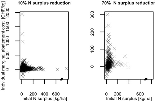
The abatement cost level at a reduction of 10% increased by 0.088 CHF with every additional kilogramme of higher N surplus (p = 0.04; r² = 0.001) (see Figure 4). The effect size and the R² were low. For the abatement cost level at a reduction of 70%, there was no significant correlation between N surplus and N abatement cost. The variation in the abatement cost increased with higher reduction of N surplus, as illustrated by some farms having more linear MACCs whereas others had increasing marginal abatement costs.

Figure 4. Marginal abatement costs of individual model agents in relation to the N surplus for a reduction of (a) 10% and (b) 70% of the initial surplus.

3.3. Cumulative marginal abatement cost curve and the price of individual transferable quota

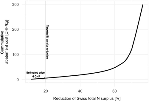
The cumulative MACC did not start at the point of origin (see Figure 5), because some agents could reduce their N surplus to a certain extent without any income losses, or even with gains. Negative individual MACCs happened as a PMP approach was considered in the optimization and the restriction of the N surplus forced the agents to optimize for their N surplus. Due to the aggregation at different price levels, the negative values were accumulated at the level of 1 CHF per kg. If we reduced the surplus by 20,000 t (this figure corresponds to a 20% N surplus reduction in Switzerland and was assumed in our NSP scenarios), we obtained a quota price of 6 CHF kg⁻¹ N (see Figure 5). The quota price increased exponentially when the N surplus reduction rose. The first tonne might be reduced by switching the farm practice to an abatement option with lower N inputs and higher ecological direct payments, whereas at higher reduction levels more costly measures, such as reducing animal numbers, were considered. To meet the agri-environmental goals for nitrate pollution and ammonia emissions, a reduction of about 50% (approximately 55,000 t) of the N surpluses would be needed (BAFU [Bundesamt für Umwelt], and BLW [Bundesamt für Landwirtschaft] 2016). The marginal costs would be about 36 CHF per kilogramme of N surplus reduction.

Figure 5. Cumulative marginal abatement cost curve for the whole agricultural sector (1 CHF ≈ 1 USD).

3.4. Effects of the distribution of certificates

The differences in N surplus reduction of the different farm types between the two trade scenarios were minor (see Figure 6d). The largest difference was in the farm type “pigs or poultry,” the only group where the “No trade” scenario had a lower N surplus than in both trade scenarios. Farms with pigs or poultry had an N surplus that was higher than average; for specialized pig and poultry farms, the N surplus was double the average. In other farms and combined arable and dairy farms, the N surplus was much higher in the “No trade” scenario. This was an effect of the change in the exit rate (Figure 6c), which influenced the farm sample and also led to a higher income for this group under the “No trade” scenario. The effect of the “Area-based” and “Grandfathering” scenarios on farm income was small (Figure 6a). Most farms achieved a slightly higher farm income in an area-based scenario than in a grandfathering distribution scheme, but a higher income than in a “No trade” scenario, expect for the already mentioned cases in other farms and combined arable and dairy farms.

Figure 6. Effects of NSP trading with distribution based on area or based on a grandfathering scheme in comparison with a default reduction of 80% of the initial N surplus on (a) average farm income and (b) average farm size (c) exit rate and (d) N surplus of different farm types.

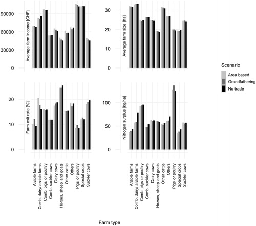
In combined suckler cow, dairy cow, sheep, goat and horse, other cattle and suckler cow farms, the farm exit rate increased from the “Area-based” to the “Grandfathering” to the “No trade” scenario. The different scenarios also had an effect on the land trade, which was indicated by the different exit rates and the different responses to the average size of the farms (Figure 6b,c). In pig and poultry farms, the average farm size was lower under the “No trade” scenario than under the “Area-based” scenario, although the exit rate was the same. These results indicate that farms were less competitive in the land market under this scenario.

In all farm types, except pig, poultry and combined pig and poultry, the average N surplus was lower than the allowance by distributed certificates, which corresponds to 80% of the average N surplus; thus, these farms sold certificates and gained a profit. In the case of pig, poultry and combined pig and poultry farms, the higher average farm income in an area-based scenario compared with the grandfathering scenario was caused by the changing farm sample due to the higher exit rate under this scenario (Figure 6b).

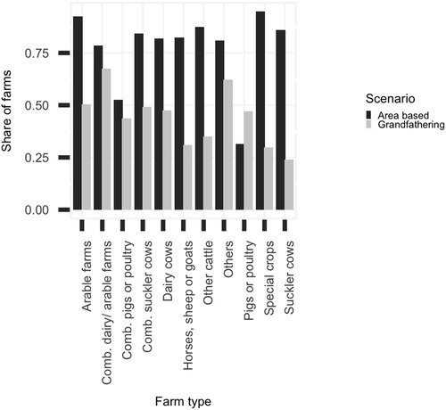
In an area-based scenario, most farms sold their certificates because their average N surplus was lower than the average N surplus of the whole sector. The only exception was pig or poultry farms; only a quarter of pig or poultry farms sold certificates and the rest bought additional certificates (Figure 7). In the grandfathering scenario, farm types with higher abatement costs tended to buy additional certificates, whereas farms with low abatement costs tended to sell them. The farm type “pigs or poultry” had a higher average N surplus in the grandfathering scenario than in the area-based distribution scheme (Figure 6d). Pig farms had to reduce their N surplus by around half to comply with their distributed N surpluses in an area-based scheme, whereas many other farm types did not have to reduce their N surplus in this scenario at all. The choice of the certificate allocation scheme had small effects on the exit rate of the different farm types. Despite the minor differences, the distribution influenced the decisions regarding land leasing and whether to give up farm activities in some cases.

Figure 7. Share of farms selling nitrogen surplus permits (NSP) in combination with a reduction in N surplus in the two NSP scenarios.

4. Discussion

4.1. Abatement costs for each farm type

The individual MACCs differed between distinct farm types. Some farms could reduce their costs by slightly reducing their N surplus, leading to negative MACCs (which could be shown due to the PMP approach). The agents showed a high variation in MACCs of N surplus in different farm types. This was also found for Swiss mountain dairy farms by Mamardashvili, Emvalomatis, and Jan (2016). Those authors assumed constant abatement costs regardless of the N surplus reduction level. However, our results showed that abatement costs increase with rising levels of N surplus reduction for most cattle farms.

4.2. Abatement costs in relation to the nitrogen surplus in the base year

The initial N surplus and the abatement costs hardly correlate for a reduction of 20%. For the 70% reduction in N surplus, no relationship was detectable. Some farms that had a high N surplus might have had low abatement costs, whereas farms with low N surplus might have had high costs. This may have affected the evaluation of the fairness of the instrument. Questions about fairness are also raised by the results from the Ramilan et al. (2011) study, which found that higher polluting farms had lower abatement costs.

4.3. Cumulative marginal abatement cost

We found that the costs for a 20% N surplus reduction are 6 CHF kg⁻¹ N. This was still more cost-efficient than an N input tax where the same level of reduction was reached with a tax of 12 CHF kg⁻¹ of N input (Schmidt et al. 2017). The input tax optimizes the input, which does not necessarily optimize the N surplus, leading to a lower cost efficiency. However, transaction costs might be higher with NSPs. Pareto-efficiency cannot be fully reached because information on marginal benefits is often not fully available (Sun, Delgado, and Sesmero 2016).

4.4. Allocation schemes

The difference between the two NSP allocation systems (land- or grandfathering-based) was only relevant for farms with pigs and poultry. These farms had a high N surplus and a high productivity per hectare.

The low impact of the allocation scheme on the exit rate is consistent with a study by Rosendahl and Storrøsten (2011) on trade in CO₂ emission certificates. Buysse et al. (2012) claim that quota systems have had an effect on structural change, although they are motivated by environmental issues. Quota systems also affect the supply chain (Wu et al. 2018). In addition, land prices can be affected by distribution of rights, especially in the land-based allocation, as farmers with low N surpluses might gain additional profit from selling rights. Whether an NSP scheme is accepted depends partly on whether society is convinced that the abatement costs are fairly distributed and partly on the administrative costs of an instrument (Stranlund and Chávez 2013).

4.5. Model limitations

Our approach to estimating N farm gate balances involved some uncertainties: 1) the estimation of N inputs based on economic data; 2) the use of constant values for N deposition and N fixation; and 3) the N content in farm products. Furthermore, farmyard manure shipments were assumed to be constant over time.

The estimation of the individual MACCs by micro-economic optimization models allowed us to depict differences between individual farms. However, we did not consider individual technical measures, long-term investments or sunk costs. This affects the estimation of the MACC. The optimization of feed to reduce N surplus was only considered in dairy production. Nitrogen- and phosphorus-reduced (NP_r) feed could reduce the N surplus of pig farms by 3–14% (calculation based on data published by Bracher and Spring 2011). Most poultry farms already use NP_r feed so further reduction was minor. Suckler cows are usually fed based on own grassland. These N flows were not explicitly considered in the N balance.

The possibility of working off-farm was not accounted for. This decision cannot be considered in the optimization as Swiss farm incomes are lower than comparable incomes (Hoop and Schmid 2013). In addition, our model did not allow us to estimate the abatement costs for switching to organic production, which affects N inputs and outputs. Hence, it was difficult to assess how the abatement costs were affected. The effects of the N restriction on prices were not considered. This assumption is reasonable because prices of agricultural products in Switzerland are dependent on import quotas. Another limitation was that the MACC was only estimated in one year. There may be changes in MACC during simulation due to the leasing of additional land.

In the agent-based approach, we yielded the potential of 3,300 heterogenous farm data leading to different MACC that allowed us to represent NSP trading. In addition, the agent-based model enabled us to estimate the effects of the policies on farm exit rates. However, the generalist farm model did not account for all the specialities of every farm. The methodology would also allow the modeling of network effects and an explicit market, which was neglected.

4.6. Policy implications

The NSP instrument can be effective in reducing N surpluses in Switzerland. However, the reduction is costly in comparison with the price for N fertilizer (∼1.13 CHF). N surpluses are a better indicator to represent a potential loss of N to the environment than are N inputs (Oenema, Kros, and de Vries, 2003). Thus, policies focusing on N surpluses might give an incentive to optimize N inputs rather than minimizing them (Bakam, Balana, and Matthews 2012). NSPs might be more cost-efficient to reduce N pollution than an N input levy (Schmidt et al. 2017), but transaction costs need to be included in the evaluation (Bakam, Balana, and Matthews 2012).

The instrument has some limitations, as it only reduces overall surplus and does not address spatial heterogeneities, which reduce effectiveness and cost efficiency (Jayet and Petsakos 2013; Kaye-Blake et al. 2019). An integrated policy mix that addresses ammonia NH₄⁺ NO₃⁻ NO_x and nitrous oxide (N₂O) is mandatory to avoid pollution swapping (Sutton et al. 2011).

There are many other options to address N pollution, for example concentration permit trading where farms exceeding their concentration permit must either transport their manure to other farms with unused rights or process the manure (Van der Straeten et al. 2011), subsidies for N reducing technology such as drag hose (Jan, Calabrese, and Lips 2017) or consumer taxes (Schmutzler and Goulder 1997).

5. Conclusion

In this study, we analyzed the abatement costs for reducing the N farm gate surplus of 3,400 Swiss farms in the FADN dataset by estimating the income reduction at different levels of surplus reduction per kg N. We then compared two different N certificate distribution scenarios: a grandfathering scheme and a scheme based on agricultural area.

Swiss farms have high variability in terms of N surplus abatement costs. Although individual marginal abatement costs can be negative, cumulative marginal abatement to meet agri-environmental goals was up to 36 CHF per kg of N surplus reduction. The individual MACC depended partly on the farm type, but the N surplus of the base year hardly explained the individual MACC. Thus, NSPs for N surplus reduction based on grandfathering might favor more polluting farms over farms with high abatement costs. However, the NSP distribution scheme had hardly any impact on the agricultural sector, except that land-based distribution would probably drive a few pig and poultry farms out of business. Nevertheless, due to the nature of N_r pollution, uniform instruments should be accompanied by a thoughtful policy mix or trading should be regionally restricted to avoid adverse effects. Policies considering N surpluses aim to approximate N use efficiency. Thus, they are more concise than policies focusing on N inputs. However, cost efficiency including transaction costs, marginal benefits and price effects needs to be further evaluated.

Acknowledgements

We are grateful to Christine Zundel from the Federal Office for Agriculture for her comments on an earlier version of the manuscript, although any errors are our own and should not tarnish her illustrious reputation. We would also like to thank seven anonymous reviewers.

Data availability

A summary of the Farm Accountancy Data Network (FADN) data that supports the findings of this study is available in Hoop and Schmid (2013). Restrictions apply to the availability of these data, which were used under license for this study. Data can be requested from Agroscope, Ettenhausen.

Disclosure statement

No potential conflict of interest was reported by the author(s).

Supplemental data

Supplemental data for this article can be accessed here.

Notes

1 The farms have already replaced a large quantity of mineral fertilisers with farmyard manure because they have to comply with the “Suisse-balance” (Jan, Calabrese, and Lips 2017).

References

- Agridea. 2013a. Deckungsbeitragskatalog 2013. Lindau: Agridea.
- Agridea. 2013b. Preiskatalog. Lindau: Agridea.
- Álvarez, F., and F. J. André. 2015. “Auctioning versus Grandfathering in Cap-and-Trade Systems with Market Power and Incomplete Information.” Environmental and Resource Economics 62 (4): 873–906. doi:10.1007/s10640-014-9839-z.
- BAFU (Bundesamt für Umwelt), and BLW (Bundesamt für Landwirtschaft). 2016. “Umweltziele Landwirtschaft: Statusbericht 2016.” In Umwelt-Wissen, edited by Bundesamt für Umwelt, 1–114. Bern: Bundesamt für Umwelt.
- Bakam, I., B. B. Balana, and R. Matthews. 2012. “Cost-Effectiveness Analysis of Policy Instruments for Greenhouse Gas Emission Mitigation in the Agricultural Sector.” Journal of Environmental Management 112: 33–44. doi:10.1016/j.jenvman.2012.07.001.
- Berntsen, J., B. M. Petersen, B. H. Jacobsen, J. E. Olesen, and N. J. Hutchings. 2003. “Evaluating Nitrogen Taxation Scenarios Using the Dynamic Whole Farm Simulation Model FASSET.” Agricultural Systems 76 (3): 817–839. doi:10.1016/S0308-521X(02)00111-7.
- Boller, B., A. Lüscher, and S. Zanetti. 2003. “Schätzung der biologischen Stickstoff-Fixierung in Klee-Gras-Beständen.” Schriftenreihe FAL 45: 47–54.
- Bracher, A., and P. Spring. 2011. “Rohproteingehalte in Schweinefutter: Bestandesaufnahme 2008.” Agrarforschung Schweiz 2 (6): 244–251.
- Busenkell, J. 2004. “Beurteilung von Agrarumweltmaßnahmen in Nordrhein-Westfalen und Rheinland-Pfalz: Einzelbetriebliche Analyse der Programme im Ackerbau.” PhD, Rheinische Friedrich-Wilhelms-Universität,
- Buysse, J., B. Van der Straeten, S. Nolte, D. Claeys, and L. Lauwers. 2012. “Optimisation of Implementation Policies of Environmental Quota Trade.” European Review of Agricultural Economics 39 (1): 95–114. doi:10.1093/erae/jbr044.
- Clò, S. 2011. “Analysis of the Allocation Rules: Do Polluters Pay under Grandfathering?” In European Emissions Trading in Practice: An Economic Analysis, Chap. 6, edited by S. P. Clò, 100-122. Cheltenham: Edward Elgar Publishing.
- Eory, V., S. Pellerin, G. C. Garcia, H. Lehtonen, I. Licite, H. Mattila, T. Lund-Sørensen, et al. 2018. “Marginal Abatement Cost Curves for Agricultural Climate Policy: State-of-the-Art, Lessons Learnt and Future Potential.” Journal of Cleaner Production 182: 705–716. doi:10.1016/j.jclepro.2018.01.252.
- Feess, E., and A. Seeliger. 2013. Umweltökonomie und Umweltpolitik. 4th ed. München: Franz Vahlen.
- Finger, R. 2012. “Nitrogen Use and the Effects of Nitrogen Taxation under Consideration of Production and Price Risks.” Agricultural Systems 107: 13–20. doi:10.1016/j.agsy.2011.12.001.
- Flisch, R., S. Sinaj, R. Charles, and W. Richner. 2009. “GRUDAF 2009: Grundlagen für die Düngung im Acker- und Futterbau.” Agrarforschung 16 (2): 1–97.
- Golub, A., T. Hertel, H.-L. Lee, S. Rose, and B. Sohngen. 2009. “The Opportunity Cost of Land Use and the Global Potential for Greenhouse Gas Mitigation in Agriculture and Forestry.” Resource and Energy Economics 31 (4): 299–319. doi:10.1016/j.reseneeco.2009.04.007.
- Hasler, B., L. Block Hansen, H. E. Andersen, and M. Termansen. 2019. “Cost-Effective Abatement of Non-Point Source Nitrogen Emissions: The effects of uncertainty in retention.” Journal of Environmental Management 246: 909–919. doi:10.1016/j.jenvman.2019.05.140.
- Hoop, D., and D. Schmid. 2013. Grundlagenbericht 2013: Zentrale Auswertung von Buchhaltungsdaten. Ettenhausen: Agroscope INH.
- Jan, P., C. Calabrese, and M. Lips. 2013. Bestimmungsfaktoren des Stickstoff-Überschusses auf Betriebsebene. Teil 1: Analyse auf gesamtbetrieblicher Ebene. Ettenhausen: Forschungsanstalt Agroscope Reckenholz-Tänikon ART.
- Jan, P., C. Calabrese, and M. Lips. 2017. “Determinants of Nitrogen Surplus at Farm Level in Swiss Agriculture.” Nutrient Cycling in Agroecosystems 109 (2): 133–148. doi:10.1007/s10705-017-9871-9.
- Jayet, P.-A., and A. Petsakos. 2013. “Evaluating the Efficiency of a Uniform N-Input Tax under Different Policy Scenarios at Different Scales.” Environmental Modeling & Assessment 18 (1): 57–72. doi:10.1007/s10666-012-9331-5.
- Kaye-Blake, W., C. Schilling, R. Monaghan, R. Vibart, S. Dennis, and E. Post. 2019. “Quantification of Environmental-Economic Trade-Offs in Nutrient Management Policies.” Agricultural Systems 173: 458–468. doi:10.1016/j.agsy.2019.03.013.
- Lengers, B., Britz, W., and K. Holm‐Müller. 2014. “What Drives Marginal Abatement Costs of Greenhouse Gases on Dairy Farms? A Meta‐Modelling Approach.” Journal of Agricultural Economics 65 (3): 579–599. doi:10.1111/1477-9552.12057.
- Mack, G., and R. Huber. 2017. “On-Farm Compliance Costs and N Surplus Reduction of Mixed Dairy Farms under Grassland-Based Feeding Systems.” Agricultural Systems 154: 34–44. doi:10.1016/j.agsy.2017.03.003.
- Mamardashvili, P., G. Emvalomatis, and P. Jan. 2016. “Environmental Performance and Shadow Value of Polluting on Swiss Dairy Farms.” Journal of Agricultural and Resource Economics 41 (2): 225–246.
- Mann, S., and S. Lanz. 2013. “Happy Tinbergen: Switzerland's New Direct Payment System/Heureux Tinbergen: Le nouveau système de paiements directs de la Suisse/Tinbergen wäre zufrieden: Das neue Direktzahlungsprogramm in der Schweiz.” EuroChoices 12 (3): 24–28. doi:10.1111/1746-692X.12036.
- Meier, B. 2000. Neue Methodik für die Zentrale Auswertung von Buchhaltungsdaten an der FAT. Tänikon: Eidgenössische Forschungsanstalt für Agrarwissenschaften und Landtechnik (FAT).
- Mérel, P., F. Yi, J. Lee, and J. Six. 2014. “A Regional Bio-Economic Model of Nitrogen Use in Cropping.” American Journal of Agricultural Economics 96 (1): 67–91. doi:10.1093/ajae/aat053.
- Möhring, A., G. Mack, and C. Willersinn. 2012. “Gemüseanbau: Modellierung der Heterogenität und Intensität.” Agrarforschung Schweiz 3 (7–8): 382–389.
- Möhring, A., G. Mack, A. Zimmermann, A. Ferjani, A. Schmidt, and S. Mann. 2016. Agent-Based Modeling on a National Scale: Experience from SWISSland. Ettenhausen: Agroscope.
- Oenema, O., H. Kros, and W. de Vries. 2003. “Approaches and Uncertainties in Nutrient Budgets: Implications for Nutrient Management and Environmental Policies.” European Journal of Agronomy 20 (1-2): 3–16. doi:10.1016/S1161-0301(03)00067-4.
- Pellerin, D., E. Charbonneau, L. Fadul-Pacheco, O. Soucy, and M. A. Wattiaux. 2017. “Economic Effect of Reducing Nitrogen and Phosphorus Mass Balance on Wisconsin and Québec Dairy Farms.” Journal of Dairy Science 100 (10): 8614–8629. doi:10.3168/jds.2016-11984.
- Ramilan, T., F. G. Scrimgeour, G. Levy, D. Marsh, and A. J. Romera. 2011. “Simulation of Alternative Dairy Farm Pollution Abatement Policies.” Environmental Modelling & Software 26 (1): 2–7.
- Rosendahl, K. E., and H. B. Storrøsten. 2011. “Emissions Trading with Updated Allocation: Effects on Entry/Exit and Distribution.” Environmental and Resource Economics 49 (2): 243–261. doi:10.1007/s10640-010-9432-z.
- Schmidt, A., M. Necpalova, A. Zimmermann, S. Mann, J. Six, and G. Mack. 2017. “Direct and Indirect Economic Incentives to Mitigate Nitrogen Surpluses: A Sensitivity Analysis.” Journal of Artificial Societies and Social Simulation 20 (4): 1–7. doi:10.18564/jasss.347.
- Schmutzler, A., and L. H. Goulder. 1997. “The Choice Between Emission Taxes and Output Taxes under Imperfect Monitoring.” Journal of Environmental Economics and Management 32 (1): 51–64. doi:10.1006/jeem.1996.0953.
- Spiess, E. 2011. “Nitrogen, Phosphorus and Potassium Balances and Cycles of Swiss Agriculture from 1975 to 2008.” Nutrient Cycling in Agroecosystems 91 (3): 351–365. doi:10.1007/s10705-011-9466-9.
- Stevens, C. J., and J. N. Quinton. 2009. “Diffuse Pollution Swapping in Arable Agricultural Systems.” Critical Reviews in Environmental Science and Technology 39 (6): 478–520. doi:10.1080/10643380801910017.
- Stranlund, J. K., and C. A. Chávez. 2013. “Who Should Bear the Administrative Costs of an Emissions Tax?” Journal of Regulatory Economics 44 (1): 53–79. doi:10.1007/s11149-013-9216-9.
- Stuhlmacher, M., S. Patnaik, D. Streletskiy, and K. Taylor. 2019. “Cap-and-Trade and Emissions Clustering: A Spatial-Temporal Analysis of the European Union Emissions Trading Scheme.” Journal of Environmental Management 249: 109352. doi:10.1016/j.jenvman.2019.109352.
- Sun, S., M. S. Delgado, and J. P. Sesmero. 2016. “Dynamic Adjustment in Agricultural Practices to Economic Incentives Aiming to Decrease Fertilizer Application.” Journal of Environmental Management 177: 192–201. doi:10.1016/j.jenvman.2016.04.002.
- Sutton, M. A., C. M. Howard, J. W. Erisman, G. Billen, A. Bleeker, P. Grennfelt, H. van Grinsven, and B. Grizzetti. 2011. The European Nitrogen Assessment: Sources, Effects and Policy Perspectives. 1st ed. Cambridge: Cambridge University Press.
- Van der Straeten, B., J. Buysse, S. Nolte, L. Lauwers, D. Claeys, and G. Van Huylenbroeck. 2011. “Markets of Concentration Permits: The Case of Manure Policy.” Ecological Economics 70 (11): 2098–2104. doi:10.1016/j.ecolecon.2011.06.007.
- Van Grinsven, H. J. M., M. Holland, B. H. Jacobsen, Z. Klimont, M. A. Sutton, and W. J. Willems. 2013. “Costs and Benefits of Nitrogen for Europe and Implications for Mitigation.” Environmental Science & Technology 47 (8): 3571–3579. doi:10.1021/es303804g.
- Verde, S. F., J. Teixidó, C. Marcantonini, and X. Labandeira. 2019. “Free Allocation Rules in the EU Emissions Trading System: What Does the Empirical Literature Show?” Climate Policy 19 (4): 439–452. doi:10.1080/14693062.2018.1549969.
- Woerdman, E., A. Arcuri, and S. Clò. 2008. “Emissions Trading and the Polluter-Pays Principle: Do Polluters Pay under Grandfathering?” Review of Law & Economics 4 (2): 565–590. doi:10.2202/1555-5879.1189.
- Wu, P., Y. Yin, S. Li, and Y. Huang. 2018. “Low-Carbon Supply Chain Management Considering Free Emission Allowance and Abatement Cost Sharing.” Sustainability 10 (7): 2110. doi:10.3390/su10072110.
- Zimmermann, A., A. Möhring, G. Mack, A. Ferjani, and S. Mann. 2015. “Pathways to Truth: Comparing Different Upscaling Options for an Agent-Based Sector Model.” Journal of Artificial Societies and Social Simulation 18 (4): 11. doi:10.18564/jasss.2862.