Response time concealed information test using fillers in cybercrime and concealed identity scenarios

ABSTRACT

The Response Time Concealed Information Test (RT-CIT) can reveal that a person recognises a relevant item (e.g., a murder weapon) among other control items, based on slower responses to the former compared to the latter ones. To date, the RT-CIT has been predominantly examined only in the context of scenarios that are very unlikely in real life, while sporadic assessment has shown that it suffers from low diagnostic accuracy in more realistic scenarios. In our study, we validated the RT-CIT in the new, realistic, and very topical mock scenario of a cybercrime (Study 1, n = 614; Study 2; n = 553), finding significant though moderate effects. At the same time (and expanded with a concealed identity scenario; Study 3, n = 250), we assessed the validity and generalizability of the filler items presented in the RT-CIT: We found similar diagnostic accuracies when using specific, generic, and even nonverbal items. However, the relatively low diagnostic accuracy in case of the cybercrime scenario reemphasizes the importance of assessments in realistic scenarios as well as the need for further improving the RT-CIT.

KEYWORDS:

• Deception
• concealed information test
• response time
• cybercrime
• filler

Undetected deception may have extremely high costs in certain scenarios, such as counterterrorism, pre-employment screening for intelligence agencies, or high-stake criminal proceedings. However, meta-analyses have repeatedly shown that without special aid and based solely on their own best judgment, people (including police officers, detectives, and professional judges) distinguish lies from truth on a level that is only just a little better than mere chance (e.g., Hartwig & Bond, 2011).

One of the potential technological aids to overcome this problem is the Concealed Information Test (CIT; Meijer et al., 2014). The CIT aims to disclose whether examinees recognise certain relevant items, such as a weapon that was used in a recent robbery, among a set of other objects when the examinees actually try to conceal any knowledge about the criminal case. The recognition of a relevant item can be detected by various means, including by responding relatively slower to relevant items when assessed with a response time-based CIT (RT-CIT). In comparison to the other types of CITs, the RT-CIT has several important advantages. First, the RT-CIT task design and the outcome evaluation is straightforward – the predictor index can be automatically calculated immediately after the completion of a test, and this requires no particular expertise. Second, it is practically without costs since it can be run on any regular computer or even on smartphones (which also makes it easily portable; Lukács et al., 2020), and also via the internet, using any modern web-browser (which also allows remote testing; Kleinberg & Verschuere, 2015). Third, while other types of CIT have been shown to be very vulnerable to fakery (e.g., National Research Council, 2003), there is increasing evidence that the RT-CIT cannot be effectively faked (Norman et al., 2020; Suchotzki et al., 2021).

However, the RT-CIT has been predominantly examined only in the context of scenarios that are very unlikely and uncommon in real life (e.g., testing participants for the recognition of their own personal name, while real CIT use is normally restricted to crime-related details; Elaad et al., 1992; Osugi, 2011). What is more, sporadic assessment has shown that it suffers from low diagnostic accuracy in more realistic scenarios (Eom et al., 2016; Matsuda et al., 2013; Wojciechowski & Lukács, 2022). Our present aim is to validate the RT-CIT in the new, realistic, and very topical mock scenario of a cybercrime, and at the same time to further optimise the RT-CIT by examining various aspects of the items presented during the task.

The RT-CIT using fillers

During the classical RT-CIT, participants classify the presented stimuli as the target or as one of several nontargets by pressing one of two keys (e.g., Meijer et al., 2016; Suchotzki et al., 2017). Typically, five nontargets are presented, one of which is the probe (the relevant item that only a guilty person would recognise) and the rest are controls, which are similar to the probe in most respects (e.g., their category membership), and thus indistinguishable for an innocent person. For example, in a murder case where the true murder weapon was a knife, the probe could be the word “knife,” while controls could be “gun,” “rope,” etc. Assuming that the innocent examinees are not informed about how the murder was committed, they would not know which of the items is the probe. The items are repeatedly shown in a random sequence, and all of them have to be responded to with the same response keys, except one arbitrary target – a randomly selected item, otherwise similar to the controls, that has to be responded to with the other response key. Since guilty examinees recognise the probe as a relevant item too, it will become unique among the controls and, in this respect, more similar to the rarely occurring target (Lukács & Ansorge, 2021; Seymour & Schumacher, 2009; Verschuere & De Houwer, 2011). Due to this conflict between instructed response classification of probes as nontargets on the one hand, and the probe's uniqueness, and thus greater similarity to the alternative response classification as potential target on the other hand, the response to the probe will be generally slower in comparison to the controls. Consequently, based on the probe-control RT differences, guilty (i.e., knowledgeable) examinees can be distinguished from innocent (i.e., naive) examinees.

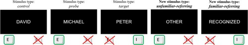
Lukács, Kleinberg, et al. (2017) have introduced the use of filler items that significantly enhanced the RT-CIT (i.e., significantly increased the accuracy of distinguishing guilty examinees from innocent ones) and that have since been used in numerous RT-CIT studies while also inspiring other test designs (e.g., Olson et al., 2020; Suchotzki et al., 2018). The inclusion of filler items was originally inspired by the Implicit Association Test (Greenwald et al., 1998), which measures the strength of associations between certain critical items to be discriminated, such as concepts or entities (e.g., various political parties), and certain attribute items to be evaluated (e.g., positive vs. negative words). The main idea is that responding is easier (and thus faster) when items closely related in their subjective evaluation (e.g., items associated with the preferred party and positive words) share the same response key. Inversely, the categorisation of the same stimuli (e.g., stimuli associated with the preferred party) will be slower when they share a response key with alternative (e.g., negative) attribute words (e.g., pain, disease). It was assumed that an analogous mechanism may be introduced in the CIT by adding probe-referring “attributes”; that is, filler items in the task. In the original studies (Lukács, Gula, et al., 2017; Lukács, Kleinberg, et al., 2017), the probes were certain personal details of the participants (their birthday, forename, etc.), which were therefore “familiar” (self-related, recognisable, etc.) to the given participant, as opposed to the controls (e.g., other dates, random animals) that were in this respect relatively “unfamiliar” (other-related, etc.). Two corresponding kinds of fillers were added to the task: (a) familiarity-referring words (“Familiar,” “Recognized,” and “Mine”) that had to be categorised with the same key as the target (and thus with the opposite key than the probe and the controls), and (b) unfamiliarity-referring words (“Unfamiliar,” “Unknown,” “Other,” “Theirs,” “Them,” and “Foreign”) that had to be categorised with the same key as the probe (and controls); see Figure 1. It was assumed that this would have a similar effect as in the Implicit Association Test: Reponses to the self-related probes (true identity details) would be even slower because they have to be categorised together with other-referring expressions (and opposite to self-referring expressions). In contrast, in case of innocents, the probes are not self-related; hence, the fillers will not slow down the responses to the probe further.

Figure 1. Example items.

Note: Examples of the possible stimulus types and corresponding required response keys (keys framed green: currently required response; keys crossed out: currently incorrect or not required response), in the Response Time Concealed Information Test (RT-CIT) with fillers. In the hypothetical scenario of suspecting the examinee to have the name “Michael,” the presentation of this name as a probe would require the same response key as any of the four control names (e.g., “David”), as well as any of the unfamiliar-referring fillers (e.g., “Other”). The opposite key would then be required for the target name (here: “Peter”) and any of the familiar-referring fillers (e.g., “Recognized”).

Subsequently, Lukács and Ansorge (2021) have examined hypotheses and mechanisms underlying the fillers’ processing, and found several significant influencing factors. First, larger enhancement was achieved when a smaller (three to six) rather than larger (reverse, six to three) proportion of fillers shared the response key with the target rather than with the nontargets (i.e., probe and controls). Second, reversing the key mapping of familiarity – and unfamiliarity-referring fillers (e.g., so that familiarity-referring fillers had to be categorised together with the probe and as alternatives to the target) robustly diminished probe-control differences, demonstrating that the enhancement indeed hinges on the semantic association via the shared key responses. Third, it was shown that nonverbal fillers (simple arrow-like characters or number strings) also lead to enhancement. This demonstrates that, in addition to semantic association, task complexity (cognitive load; due to more items in the task) can also contribute to the enhancement of the probe-control RT difference (see also Hu et al., 2013; Visu-Petra et al., 2013).

RT-CIT in crime scenarios

There are important questions still in need of further research: in particular, what the optimal arrangement of fillers is and how generalisable the impacts of the fillers are to scenarios other than autobiographical details. RT-CIT studies very often use such central autobiographical details, such as participants’ own personal names, even though real police investigations typically involve crime-related items (e.g., Elaad et al., 1992; Osugi, 2011). The classic RT-CIT seems to underperform in mock crimes, in some studies not even having achieved statistical significance (Eom et al., 2016; Matsuda et al., 2013). This issue is exacerbated by the likely low salience of minor or incidentally acquired details during a crime, which also generally decreases the diagnostic accuracy of the RT-CIT for telling truly guilty suspects from innocents (e.g., Rosenfeld et al., 2006; Verschuere et al., 2015).

One reason for these problems are the many different forms of memory involved in criminal acts, not all of which reflect intentional encoding and not all of which are of an explicit or enduring nature (e.g., Peth et al., 2012; Swanson et al., 2021). A particularly interesting domain is the memory for details related to cybercrimes (e.g., stolen passwords and other confidential data). Cybercrime in the past decades has come to carry enormous and ever-increasing impact in the world (e.g., Broadhead, 2018), with mere preventive action costs amounting to hundreds of billions of dollars yearly world-wide (Anderson et al., 2013). However, the (criminal) usage of data obtained on the internet may be tracked down less easily or lead to prosecution less easily (Smith et al., 2004). This would also correspond to a particularly lower relevance of memory for the critical information: a lower risk of harmful consequences of the disclosure of its knowledge. Data (to be) criminally used or obtained on the internet are also typically of short-term use only, as the corresponding details (e.g., stolen passwords or security codes) are usually taken out of service once a fraud has been detected. As a consequence, they are also not relevant for transfer into permanent memory. A related particular limitation is that there are typically no direct physical objects, such as a murder weapon or any part of the crime scene that could be used as probes; the incriminating information is restricted to the digital sphere. Therefore, altogether, it is an open question how well the methods developed for the detection of concealed memory in general work in this particular context. We addressed this in the present research by introducing a simulated cybercrime scenario in an online experiment.

Some previous CIT studies have gone to great lengths to create more realistic scenarios of testing for incidentally acquired details (Meixner & Rosenfeld, 2014; Norman et al., 2020) – however, this requires extensive resources and it is uncertain to what degree the researchers succeeded in creating believable simulations. Online research would allow inexpensive and extremely efficient data collection, but, to date, the only options for online RT-CIT experiments have been using either autobiographical details (e.g., Kleinberg & Verschuere, 2015) or rehearsed “imaginary crime” details, where participants are effectively just instructed that they should memorise the given details (e.g., Wojciechowski & Lukács, 2022). In contrast, many examples from the huge domain of cybercrimes offer themselves rather easily to a realistic simulation in online experiments. In the mock cybercrime scenario that we introduce in the present studies, participants infiltrate an email account, search for and find credit card details, and finally use these details to perform a (simulated) money transaction.

This is, of course, still not equivalent to a real crime: Participants are clearly aware that they are taking part in an experiment and that their “crime” is a simulation. Even so, to our knowledge, such a mock crime is the most realistic implementation in an online experiment to date. What is more, even when lab-based studies are more immersive (e.g., physically stealing an object), they are also disadvantaged by the clear awareness of the physical presence of an authoritative, and typically familiar, supervisor and surroundings. Our online mock cybercrime happens under far greater anonymity. Most importantly, the participants’ identity, recruited via online platforms, is completely unknown and unknowable to the researchers. However, even the researchers are unknown to the participants and the online experiment could even be a sham: Anyone could set up a website for a supposed experiment and purport to be a researcher. In this way, there is not even any direct assurance for the participant that the procedure happens in an experimental context, and it would in fact be possible to actually commit a cybercrime (assuming that the study call is a fake front to the purported researchers’ illegal activity). Hence, altogether, it may even be argued that this scenario is, at least in some respects, more realistic than any other previous mock crime used for the RT-CIT.

Study structure

In a series of three studies, apart from introducing the cybercrime scenario, we tested several hypotheses related to the filler items in the RT-CIT. This was done to investigate whether the fillers in the RT-CIT hold promise (for increasing probe-control differences) under more realistic (mock) crime conditions. The different hypotheses of the studies are explained in more detail in the introductions preceding each study. In Study 1, using the cybercrime scenario with a one-day interval between the crime and the testing, we tested the potential difference between different filler types (verbal vs. nonverbal vs. mixed), along with the effect of omitting nontarget-fillers from the task. In Study 2, using another cybercrime scenario but without any delay between the crime and the testing, we examined the effect of having greater versus smaller numbers of different filler words, along with the effect of having greater versus smaller proportions of target fillers. Finally, in Study 3, using a hidden identity scenario (autobiographical details as probes), we tested the effect of more generic versus more specific fillers. All statistical tests followed our preregistrations, except where we explicitly note otherwise.

Study 1

It is known that reverse mapping of familiarity-related fillers diminishes the fillers’ enhancing effect. However, it is unknown if the original mapping of familiarity-related word fillers outperforms nonverbal fillers. Nontarget fillers especially raised our doubts: While target filler words can quite clearly refer to the probe’s meaning, familiarity or relevance, words do not seem to capture the opposite of these concepts so easily. Actually, the mere fact that words have meaning makes them, in a sense, meaningful, and thus target-similar. Therefore, nontarget fillers in particular may better be replaced by nonverbal items. Hence, three arrangements seem worthy of investigation: (a) all fillers verbal, (b) all fillers nonverbal, and (c) target fillers verbal and nontarget fillers nonverbal. What is more, given the hypothesised lack of meaning or relevance of nontarget fillers, an additional question is whether, in any of these cases, removing nontarget fillers altogether makes any difference. At the same time, it is to be kept in mind that these additional nontarget items contribute to task complexity, a factor with the potential to enhance the probe-control difference and whose reduction may, thus, be detrimental to the RT-CIT’s diagnostic accuracy.

Hence, in this first study, we want to see (a) how verbal and nonverbal fillers as well as both combined compare, and (b) whether nontarget fillers are necessary at all. At the same time, the mock cybercrime scenario is introduced and validated.

Method

Participants

Participants were recruited via the online crowdsourcing platform Prolific (https://www.prolific.co/), selected as (self-reportedly) monolingual native English speakers born and currently residing in the United States. They were rewarded 3.00 GBP for the two-part and altogether about 25 min long experiment.

As preregistered, we opened an initial 100 slots in each of the three experimental groups and subsequently opened additional 40 slots per group until we passed 200 valid participations per group. Early stopping of collection would have been based on the criterion of the Bayes factors (BFs; with default r-scale of 0.707) reaching a minimum of 5.0 in support of either difference or equivalence for the t-tests for reaction time (RT) mean probe-control differences between the “condition with the highest mean probe-control difference” and each of the other conditions. However, this condition was never fulfilled.

The full sample included 781 participants. We excluded 150 participants who did not select at least three out of the four probes (“incriminating” details) correctly at the end of the test. Furthermore, we excluded data from 17 participants who had, within their experimental group, an accuracy rate further than three interquartile ranges (IQR) distance from the lower bound of the IQR, for any of the following item types: (a) nontargets (probe and controls merged), (b) targets, and (c) fillers (all fillers merged). This left the following: Verbal condition, 204 subjects (age = 29.8 ± 7.4; 45% male), Nonverbal condition, 202 subjects (age = 30.9 ± 8.0; 53% male), Mixed condition, 208 subjects (age = 31.3 ± 7.7; 44% male).

The ratios of those who started the second part of the experiment but subsequently dropped out (Zhou & Fishbach, 2016) were very low (for an online experiment) in all conditions: 4.07% for Verbal, 1.91% for Nonverbal, and 1.85% for Mixed.

Procedure

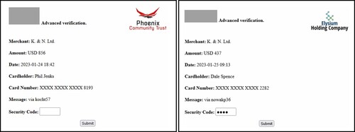
The experiment consisted of two parts, with an interval of about 24 h. The first part involved a simulated cybercrime which took about 5 min. Namely, participants were redirected to a separate website where they were (1) asked to log in to an email account with “stolen” login information, (2) look for any credit card information among the messages, and (3) provide these details on the same website in order to complete a transaction of “stealing” money from the given bank account. A demo version of the website is available via https://np36kt57.github.io/¹; see also Figure 2. For the purpose of the experiment, though using fake names, two otherwise real and fully functioning email accounts were created at the official webmail server of the University of Vienna (https://www.univie.ac.at/ZID/webmail/).² The inboxes were filled months in advance with spam and other fake personal correspondence to make them appear realistic. Among the messages, there was one that contained all necessary information for a bank card (personal name, bank name, credit card number, expiration date, PIN). Having found the details, it had to be provided on the above-linked website. Subsequently, participants received a popup to confirm a money transaction (providing the PIN once more) using a layout and mechanism resembling those of real credit card transactions. Finally, they were shown a success message, which repeated all relevant incriminating details. Returning to the experimental website, participants were reminded not to forget to complete the second and last part the next day at around the same time (after a minimum of 21 and a maximum of 27 h).

Figure 2. Screenshots of the transaction prompt.

Note: Screenshots of the transaction prompt; one of each of the two bank versions. (In the right panel’s screenshot, the security code is filled in.) On submitting the information, the browser window activates a “screen lock” and a “wait cursor” for a short while (as typical of real instances of such operations) and then returns either a confirmation message, or, in case of incorrect details, an error message. The card company logos are masked here (in gray) to avoid copyright issues.

Each participant’s navigation between the different websites was recorded with timestamps to ensure that they complied with the instructions, and participants could not continue otherwise. The login information was stored in a secure database that could only be accessed once by each participant. This access was recorded, and the same participant could only continue with the corresponding email account’s information and within the given time limit.

In the second part, the participants completed an RT-CIT using four incriminating details as probes (in each case one of two versions, corresponding to the given infiltrated email account): the login name of the email account (kocht57 or nowakp36); the name of the bank (Phoenix Community Trust or Elysium Holding Company); the personal name of the bank account holder (Phil Jenks or Dale Spence³); and the credit card PIN (5288 or 4377). The targets and controls were chosen as items of similar length in the same category, indistinguishable for a person uninformed of the relevant ones (e.g., langen92, schrobh84, etc., for login names; Vertex Corporation Banks, Zenith National Holdings, etc., for bank names).⁴ See Table 1 for two exemplary complete sets of all these target and nontarget items in the RT-CIT. Participants were asked in advance to deny having stolen the details and imagine themselves in a situation where they would actually want to “beat” the lie detection test in order to seem innocent.

Table 1. Examples for main item types.

Item Type	Example 1	Example 2	Correct Key
Target	Tim Howe	huberm94	#I
Probe	Phil Jenks	nowakp36	#E
Control	Ray Snell; Neil Rand; Gene Falk; Ralph Croft	mullerf27; schrobh84; kugele41; bohmej58	#E

Note: Two examples sets of target and nontarget (probe and control) items, one with personal names and one with email login usernames. These items always have this same structure and response requirements in all experiments.

Task design

For the RT-CIT, there was one three-level between-subjects factor and one two-level within-subject factor. The between-subjects factor “Filler Type” concerns three types of fillers: (a) verbal (importance-related fillers), (b) nonverbal (number string or arrow symbol fillers), and (c) mixed (verbal target-side fillers, but nonverbal nontarget-side fillers). The verbal target fillers were: “Meaningful,” “Crucial,” “Recognized”; while the verbal nontarget fillers were: “Unimportant,” “Insignificant,” “Other,” “Random,” “Unfamiliar,” “Irrelevant.” Nonverbal fillers were chosen randomly as either numbers or arrow-like symbols (for details, see Lukács & Ansorge, 2021). Regarding the numbers, the targets were always composed of the digits “1,” “2,” or “3,” while the nontargets were always digits between “4” and “9” (e.g., the items “11111,” “2222,” and “333333” had to be categorised with one key, while “999999,” “8888,” etc., had to be categorised with the other key). Regarding the arrow symbols, we used random combinations of arrowhead-like symbols (Unicode symbol characters), that were to be categorised with the key corresponding with the direction indicated by the symbols. For example, the item “＜<{⧼❮〈” had to be categorised with the response key on the left, and the item “＞❯>〉” had to be categorised with the response key on the right. Both number and arrow items matched the verbal fillers in character lengths. For an overview of all filler types, see Table 2. The within-subject factor “Nontarget-Fillers” had two conditions: (a) nontarget-side fillers present and (b) nontarget-side fillers absent (see further details of the trial arrangement below).

Table 2. Filler types in Study 1.

Item Type	Nonverbal	Mixed	Verbal	Correct Key
Filler-T	1111111111; 2222222222; 3333333 (or: ＞❯＞})＞⦔>⧽〉; >)＞>❯⧽〉’; ⧽)}〉⧽⦔＞＞❯>)	Meaningful; Crucial; Recognised		#I
Filler-NT	44444444444; 55555; 666666; 7777777777777; 8888888888; 9999999999 (or: ⦓{<＜〈⦓❮＜(⧼; <(<❮〈＜⦓<{＜⧼; etc.)		Unimportant; Insignificant; Other; Random; Unfamiliar; Irrelevant	#E

Note: Examples for the different filler types in the three conditions (Nonverbal, Mixed, Verbal) in Study 1. In the study, the character lengths of the given number and arrow fillers varied randomly but always matched one of each verbal filler; the order of the arrow symbols was also random. The verbal fillers were always the same. In one half of each Response Time Concealed Information Test (RT-CIT), nontarget fillers were absent. Filler-T = Target filler; Filler-NT = Nontarget filler.

During the RT-CIT, the items were presented one by one in the centre of the screen, and participants had to categorise them by pressing one of two keys (E or I) on their keyboard. They had to press Key I whenever a target or a target filler appeared, while they had to press Key E whenever the probe, a control, or a nontarget filler appeared. The inter-trial interval (i.e., between the end of one trial and the beginning of the next) always randomly varied between 500 and 800 ms. In the case of a correct response, the next trial followed. In the case of an incorrect response or no response within the given time limit, a caption stating “WRONG” or “TOO SLOW,” respectively, appeared in red colour below the stimulus for 500 ms, followed by the next trial.

The main task was preceded by three practice blocks. In the first practice block, all filler items were presented twice, hence, altogether 18 items. In the event of too few valid responses, the participants received corresponding feedback, were reminded of the instructions, and had to repeat the practice task. The requirement was a minimum of 80% valid responses (i.e., pressing of the correct key between 150 ms and 1 s following the display of an item) for each of the two filler types.

In the second practice block, the probe, the target, and the four controls of the given type (e.g., bank name or PIN) of the upcoming first main block (collection of data to be used in our analyses) were presented once, and participants had plenty of time (10 s) in each trial to choose a response. However, each trial required a correct response. In the event of an incorrect response, the participant immediately received corresponding feedback, was reminded of the instructions, and had to repeat this practice. This guaranteed that the eventual differences (if any) between the responses to the probe and the responses to the controls were not due to misunderstanding of the instructions or any uncertainty about the required responses in the eventual task.

In the third and final practice block, again all items were presented once, but the response deadline was again short (1 s) and a certain rate of mistakes was again allowed. In the event of too few valid responses, the participants received corresponding feedback, were reminded of the instructions, and had to repeat the practice block. The requirement was a minimum of 60% valid responses (pressing of the correct key between 150 ms and 1 s following an item) for each of the following item types: target filler, nontarget filler, target, or nontargets (probe and controls together).

The first half of the main blocks randomly either all contained or all did not contain nontarget fillers (within-subject factor Nontarget-Fillers), while the second half had the opposite condition (not containing or containing nontarget fillers respectively). Each of these two halves was composed of four blocks, each including one of the detail types (login name, bank name, personal name, and PIN; with the same order of types in each half). Each new block was preceded by another round of short practice block that was like the second practice round at the beginning (each item requiring a correct response within 10 s), with the probe, target, and controls of the upcoming block.

In each block, each probe, control, and target was repeated nine times (hence, nine probe, 36 control, and 9 target trials in each block). The order of these items was randomised in groups: first, all six items (one probe, four controls, and one target) in the given category were presented in a random order, then the same six items were presented in another random order (but with the restriction that the first item in the next group was never the same as the last item in the previous group). Fillers were placed among these items in a random order, but with the restriction that a filler trial was never followed by another filler trial. In case of nontarget fillers present, each of the nine fillers preceded each of the other items (probes, targets, and four controls) exactly one time in each two consecutive blocks.⁵ Thus, 9 × 6 = 54 fillers were presented per each pair of two consecutive blocks, and 54 out of the 108 other items were preceded by a filler. In case of nontarget-side fillers absent, in each double-block of 118 items, there were 10 target-side fillers. Each probe and control was preceded by two such target-side fillers. This way the proportion of target-side items (targets and target-side fillers) versus nontarget items (probes, controls, and, if any, nontarget-side fillers) in the task remains similar in the two conditions: 36–162 (22.2%) and 28–118 (23.7%).

At the end of the test, participants were presented with all probes, targets, and controls in the task, grouped per detail category (bank names, PIN, etc.), and were asked to select the probes; that is, the “incriminating” details from the simulated crime (while assuring them that we know that they “committed” the crime).

Data analysis

For the main questions, the dependent variable is the probe-control correct RT mean difference (probe RT mean minus control RT mean, per each participant, using all valid trials). The detail types (e.g., bank name, PIN) were merged.

For all analyses, RTs below 150 ms were excluded. For RT analyses, only correct responses were used. Accuracy was calculated as the number of correct responses divided by the number of all trials (after the exclusion of those with an RT below 150 ms). All analyses were conducted in R (R Core Team, 2020; using the R packages MBESS by Kelley, 2019; ez by Lawrence, 2016; neatStats by Lukács, 2021b; bayestestR by Makowski et al., 2019; BayesFactor by Morey & Rouder, 2018; ggplot2 by Wickham, 2016).

To demonstrate the magnitude of the observed effects, for F-tests we report generalised eta squared (${\eta }_G^2$) and partial eta squared (${\eta }_p^2$) with 90% CIs (Lakens, 2013). We report Welch-corrected t-tests (Delacre et al., 2017), with corresponding Cohen’s d values as standardised mean differences and their 95% CIs (Lakens, 2013). We used the conventional alpha level of .05 for all statistical significance tests.

We report Bayes factors (BFs) using the default r-scale of 0.707 (Morey & Rouder, 2018). In case of analyses of variance (ANOVAs), we report inclusion BFs based on matched models (Makowski et al., 2019). The BF is a ratio between the likelihood of the data fitting under the null hypothesis and the likelihood of fitting under the alternative hypothesis (Jarosz & Wiley, 2014; Wagenmakers, 2007). For example, a Bayes factor (BF) of 3 indicates that the obtained data is three times as likely to be observed if the alternative hypothesis is true, while a BF of 0.5 indicates that the obtained data is twice as likely to be observed if the null hypothesis is true. Here, for more readily interpretable numbers, we denote Bayesian factors as BF₁₀ for supporting the alternative hypothesis, and as BF₀₁ (meaning: ${\displaystyle \frac{1}{B{F}_{10}}}$) for supporting the null hypothesis. Thus, for example, BF₀₁ = 2 (or ${\displaystyle \frac{1}{0.5}}$) indicates that the obtained data is twice as likely under the null hypothesis than under the alternative hypothesis. Typically, BF = 3 is interpreted as the minimum likelihood ratio for “substantial” evidence for either the null or the alternative hypothesis (Jeffreys, 1961).

Diagnostic accuracy

There are a number of ways to measure diagnostic accuracy. The most straightforward is arguably the overall correct detection rate (CDR): in the present context, the number of correctly classified guilty and innocent examinees divided by the number of all guilty and innocent examinees. The CDR is obtained by using a specific cutoff that decides whether a given value (depending on whether it is below or above the cutoff) indicates guilty or innocent classification. For example, in the RT-CIT, persons with probe-control RT mean differences above the cutoff of 30 ms may be classified as guilty (due to having recognised the relevant probe item), and those below the cutoff as innocent. However, the optimal cutoff value is arbitrary in each study and does not necessarily generalise well to other scenarios (Lukács & Specker, 2020).

As an alternative, one very popular and widely used diagnostic accuracy measure for binary classification is the area under the curve (AUC) of a receiver operating characteristic (ROC; Green & Swets, 1974). The AUC is based on a comparison of two distributions of all predictor values (e.g., the distributions among guilty and among innocent participants). A ROC curve can be constructed by plotting the true positive rates (ratio of correctly classified guilty individuals) as a function of false positive rates (ratio of incorrectly classified innocent individuals) across all possible cutoff points. The AUC is the area under this ROC curve. The AUC can range from 0 to 1, where .5 means chance level classification, and 1 means flawless classification (i.e., all guilty and innocent suspects can be correctly categorised based on the given predictor variable, at a given cutoff point). Although the AUC is less straightforward to interpret than CDR, it has the advantage of being well generalisable (e.g., Fawcett, 2006).

To calculate illustrative AUCs for probe-control RT mean differences as predictors, we simulated control groups for the RT data from each of the four possible conditions, using 1,000 normally distributed values with a mean of zero and an SD derived from the real data (from each condition) as SD_real × 0.5 + 7 ms (which has been shown to very closely approximate actual AUCs; Lukács & Specker, 2020; the related function is available in the analysis codes uploaded to the OSF repository). These simulated AUCs are just approximations for illustration, and we do not use them for any of our statistical tests.

Here, we also provide some brief examples to give a practical idea about the relations, in case of the RT-CIT, among (a) the AUCs; (b) the CDRs, and (c) the raw probe-control RT differences. Assuming (based on the meta-data by Lukács & Specker, 2020), for guilty examinees, a mean probe-irrelevant RT difference of 14.5 ms (similar to the current results, see below), an SD of 33.6, and, for innocent examinees, an SD of 23.5 (and a mean of zero), the CDR is .64 and the AUC is .62. With SDs unchanged, a 6.7 ms increase of guilty probe-irrelevant RT difference to 21.2 ms would result in a CDR of .70 (a gain of .06) and an AUC of .66 (a gain of .04). A further 6.7 ms increase of probe-irrelevant RT difference to 27.9 ms would result in a CDR of .75 (a gain of .05) and an AUC of .70 (a gain of .04). In sum, differences of about 7 ms in probe-control RT differences indicate about 5% change in diagnostic accuracy. Given the difficulty in translating the results of highly controlled experimental scenarios to real life scenarios with likely far more statistical noise in the data, we find this 7 ms difference (equivalent to a Cohen’s d of ca. 0.5) to be a reasonable minimum effect size of interest (e.g., Lakens et al., 2018).

Results

Aggregated means of RT means and of probe-control RT differences for the different stimulus types in each condition are given in Table 3; the probe-control differences are also depicted in Figure 3.

Figure 3. Probe-control response time differences per condition in Study 1.

Note: Probe-Control Response Time Differences per Condition in Study 1. Means and 95% CIs of individual probe-control RT differences. NT-Fillers=Nontarget fillers.

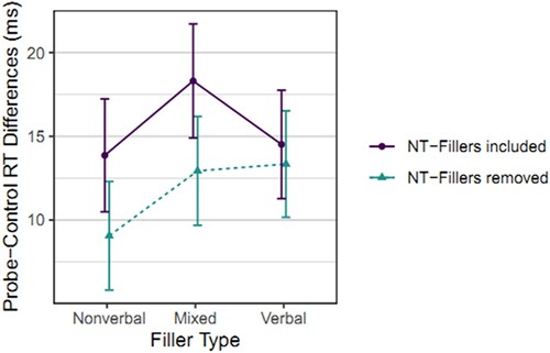
Table 3. Reaction time means per condition, in Study 1.

	Nonverbal		Mixed		Verbal
	NT	No NT	NT	No NT	NT	No NT
Probe	500 ± 68	465 ± 65	499 ± 67	477 ± 66	498 ± 62	472 ± 67
Control	486 ± 60	456 ± 57	481 ± 57	464 ± 57	483 ± 55	459 ± 59
Target	565 ± 61	521 ± 58	559 ± 54	530 ± 52	567 ± 54	527 ± 60
NT-Filler	512 ± 70		459 ± 51		557 ± 61
T-Filler	552 ± 66	531 ± 60	569 ± 53	556 ± 54	604 ± 57	569 ± 64
P – C	13.9 ± 24.4	9.1 ± 23.5	18.3 ± 25.1	12.9 ± 23.9	14.5 ± 23.6	13.3 ± 23.2
AUCsim	.659	.603	.716	.648	.669	.661

Note: Means and SDs (in the format of M ± SD) for individual reaction time (RT) means; for Probe (incriminating credit card details), Control (other, irrelevant details), Target (the designated control details that require a different response), P – C (individual probe minus control RTs). T-Filler = Target filler; NT-Filler = Nontarget filler; No NT: Nontarget fillers not included; AUC_sim: simulated Area Under the Curve.

The two-by-three ANOVA on the Nontarget-Fillers and Filler Type factors showed a significant and robust Nontarget-Fillers main effect (larger probe-control differences with nontarget fillers included), F(1, 611) = 11.53, p = .001, ${\eta }_p^2$ = .019, 90% CI [.005, .040], ${\eta }_G^2$ = .006, BF₁₀ = 17.59, no significant Filler Type main effect F(2, 611) = 2.34, p = .097, ${\eta }_p^2$ = .008, 90% CI [0, .021], ${\eta }_G^2$ = .005, BF₀₁ = 5.76, and substantial evidence for the lack of interaction, F(2, 611) = 1.39, p = .250, ${\eta }_p^2$ = .005, 90% CI [0, .015], ${\eta }_G^2$ = .002, BF₀₁ = 14.26.

As preregistered, follow-up t-tests focus on the condition with the highest probe-control RT mean differences, the Mixed fillers with the inclusion of nontarget fillers, comparing it with the rest of the conditions. Due to the lack of interaction and strong and consistently clear within-subject effect (see Figure 3), we deem the condition without nontarget fillers altogether significantly inferior and compare only the different between-subjects groups. The Mixed condition did not significantly outperform either of the other conditions, Verbal condition: nominal difference of 3.79 ms, 95% CI [−0.92, 8.51], t(409.3) = 1.58, p = .115, d = 0.16, 95% CI [−0.04, 0.35], BF₀₁ = 2.75; Nonverbal condition: nominal difference of 4.45 ms, 95% CI [−0.36, 9.25], t(408.0) = 1.82, p = .070, d = 0.18, 95% CI [−0.01, 0.37], BF₀₁ = 1.86. Nonetheless, the very small magnitudes of the lower limits of the 95% CIs (−0.92 and −0.36 ms) indicate that it is very unlikely that either the Verbal or the Nonverbal condition is substantially better than the Mixed condition.

Secondary analysis

The simulated AUCs for different items types were: .689 for bank names, .622 for personal names, .576 for login names, and .532 for PINs. To test whether perhaps using arrows versus numbers makes a difference in the (nominally best performing) Mixed condition, we compared their respective probe-control RT mean differences in an explorative way, with a not preregistered t-test, and found a small nominal advantage for using arrows, but with support only for equivalence, 0.96 ms, 95% CI [−4.63, 6.54] (Mean ± SD = 15.97 ± 22.61 vs. 15.02 ± 17.52), t(182.2) = 0.34, p = .736, d = 0.05, 95% CI [−0.22, 0.32], BF₀₁ = 6.25.⁶

Study 2

We found no statistically significant differences, but the Mixed version seems to have been sufficiently proven as not inferior to the Verbal and Nonverbal versions. In other words, the Mixed version is very unlikely to perform worse than the others and it might even perform better. In addition, all other things being equal, there seems to be no compelling reason against using the Mixed fillers rather than Verbal or Nonverbal. In contrast to Verbal fillers, Mixed fillers have the advantage that there is no need for the potentially complicated selection of six words for the irrelevance – or meaninglessness-referring nontarget fillers; instead, simple nonverbal characters can be used. As compared to the Verbal fillers, it does only require selecting three relevance – or meaningfulness-referring target fillers. However, in our experience (with implementing various fillers in various languages; e.g., Lukács et al., 2021), this latter task is not too difficult, partly because only three fillers are needed, and partly because, in contrast to irrelevance-referring words, there are typically several obviously suitable choices for relevance-referring ones. Hence, the Mixed version does not substantially complicate practical implementation as compared to the purely Nonverbal version. Therefore, altogether, while this topic might deserve further research, we decided to use the Mixed version for all remaining studies for the present article.

Originally, the introduction of filler items to the RT-CIT was also intended to increase task complexity, in particular by having more variants of target-side items (four instead of one) for the participants to look out for (Lukács, Kleinberg, et al., 2017, p. 3). However, this modification at the same time inherently increased the number of different items in the test as well. The particular aspect of variety was later addressed in a dedicated study where more variants of targets (i.e., control-like items; four instead of two, with unchanged overall number of presentations) also enhanced the RT-CIT (Suchotzki et al., 2018). This inspired us to propose further enhancements of the RT-CIT with fillers by adding more variety in target-side items, namely, having six instead of three fillers (so that, together with the target, there would be seven instead of four target-side items; with unchanged overall number of presentations). Examining this scenario also contributes to another line of investigations, namely, the potential prevention of detrimental habituation effects in the RT-CIT (Lieblich et al., 1974; Lord & Novick, 2008; Lukács, 2022): There is some tentative evidence that introducing more varied items may counter the decrease of probe-control differences across time (see online Appendix A in Lukács, 2022), but this has not been conclusively demonstrated thus far.

The fact that a smaller proportion of target relative to nontarget fillers (three to six) is important for the enhancement seems to suggest the potential of further enhancement by the further reduction of the targets’ proportion. The uniqueness of target-category items is assumed to be a factor in eliciting response conflict in case of the (in this respect similar) probes among the controls, thereby, contributing to larger probe-control differences (Lukács & Ansorge, 2021; Rothermund & Wentura, 2004; Suchotzki et al., 2015). Hence, a reduction of the overall frequency of target-side trials may further increase probe-control differences.

All in all, in this second study, we wanted to see whether probe-control differences can be increased by (a) lowering the proportion of target-side items, and/or (b) showing a greater variety of target-side fillers. We used the same mock cybercrime scenario as in Study 1, except that there was no delay between the crime and the testing.

Method

Participants

Participants were recruited via Prolific as in Study 1. They were rewarded 3.50 GBP for the 25–30 min experiment. As preregistered, we opened an initial 130 slots in each of the two experimental groups (altogether 260). Since the one-sided t-tests gave strong evidence (BF > 10) that smaller target-side item proportion (see below) does not lead to increased probe-control RT differences, this condition was dropped from the experiment for the rest of the data collection and replaced with the other within-subject condition (hence, same condition repeated twice for all remaining participants).

Since our other stopping condition (BF > 5 for all comparisons of the condition with the highest mean probe-control difference) was never fulfilled, we opened 85 additional slots for each of the two groups (altogether 170) two times, as per preregistration. Hence, the final sample included 600 participants. We excluded 28 participants who did not select at least three out of the four probes correctly at the end of the test. Furthermore, we excluded data from 19 participants who had, within their experimental group, an accuracy rate further than three interquartile ranges (IQR) distant from the lower bound of the IQR, for any of the following item types: (a) nontarget items (probe and controls merged), (b) targets, and (c) fillers (all fillers merged). This left the following: Regular condition, 276 subjects (age = 27.6 ± 7.5; 39% male, 61% female), Varied condition, 277 subjects (age = 27.8 ± 7.6; 39% male, 61% female); within which the initial batch of 260 opened slots resulted in, in Regular, 118 subjects (age = 27.1 ± 7.3; 40% male, 60% female), and, in Varied, 113 subjects (age = 27.9 ± 7.8; 39% male, 61% female).

The ratios of those who started the RT-CIT but subsequently dropped out were again relatively low in both conditions: 3.78% for Varied, 4.23% for Regular.

Procedure

The procedure was the same as in Study 1, aside from the modifications highlighted in this next section.

Though including a delay between crime and testing is more realistic, we assume that it does not have substantial influence on the differences between the main (probe-control difference) outcomes of the experimental conditions. Therefore, to make it more likely that participants remember the detail, and thereby, reduce related exclusions (which were rather high in Study 1; 150 out of 781), here, the experiment consisted of a single part, with RT-CIT immediately following the simulated crime (which indeed resulted in a much higher rate of recall, with only 28 necessary exclusions out of 600).

All tests used the Mixed filler design from Study 1 (nonverbal nontarget fillers, but verbal target fillers). There was one two-level between-subjects factor, and one two-level within-subject factor. For the between-subjects factor “Variety,” the participants in the Varied condition performed the RT-CIT with six different target filler expressions (“Relevant,” “Recognized,” “Important,” “Familiar,” “Crucial,” “Significant”). Those in the Regular (conventional) condition, had three different target fillers, similar to previous studies and Study 1 of the present article, except that in this case, at the beginning of each test, they were randomly chosen out of the six fillers included in the other condition. The six fillers were altogether presented the same number of times as the three fillers, so that the number of target filler trials remained the same overall, only there was more variety in the used expressions in the former case. For the within-subject factor “Proportion,” in one half of each test, the number of target-side items (target fillers as well as targets) were reduced to 10 target-side fillers instead of 18, and to 10 targets instead of 18, counting per each of two blocks (consisting altogether of 90 probe and control items).

Results

Aggregated means of RT means and probe-control differences for the different stimulus types in each condition, are given in Table 4.

Table 4. Reaction time means per condition, in Study 2.

	Regular		Varied
	More T	Less T	More T	Less T
Probe	494 ± 58	474 ± 60	510 ± 65	480 ± 67
Control	474 ± 52	455 ± 53	486 ± 57	462 ± 57
Target	554 ± 50	553 ± 53	566 ± 52	557 ± 53
NT-Filler	444 ± 47	430 ± 48	456 ± 54	435 ± 53
T-Filler	557 ± 47	566 ± 52	572 ± 49	583 ± 47
P – C	20.1 ± 23.7	18.9 ± 25.1	23.7 ± 24.9	18.0 ± 26.7
AUCsim	.743	.711	.769	.699

Note: Means and SDs (in the format of M ± SD) for individual reaction (RT) means; for Probe (incriminating credit card details), Control (other, irrelevant details), Target (the designated control details that require a different response), P – C (individual probe minus control RTs). T-Filler = Target filler; NT-Filler = Nontarget filler; AUC_sim: simulated Area Under the Curve. More T = relatively larger proportion of target-side items; Less T = relatively smaller proportion of target-side items.

The two-by-two ANOVA on the Variety and Proportion factors (using the initial sample of 231 participants) showed no significant Variety main effect, F(1, 229) = 1.18, p = .278, ${\eta }_p^2$ = .005, 90% CI [0, .031], ${\eta }_G^2$ = .004, BF₀₁ = 3.80; larger probe-control differences in case of more targets (Proportion main effect), F(1, 229) = 6.04, p = .015, ${\eta }_p^2$ = .026, 90% CI [.003, .068], ${\eta }_G^2$ = .008, BF₁₀ = 1.78; and a significant interaction (larger Proportion effect in case of more Varied fillers; Figure 4), F(1, 229) = 4.40, p = .037, ${\eta }_p^2$ = .019, 90% CI [.001, .057], ${\eta }_G^2$ = .006, BF₁₀ = 1.09; see Table 4 and Figure 4. The interaction indicates a larger difference between less versus more targets in the Varied condition as compared to the Regular condition (where the difference is near zero). However, regarding the proportion of targets: We were interested in whether fewer targets increase probe-control differences compared to the conventional version with more targets. This was clearly not the case: Fewer targets resulted in at least nominally lower probe-control differences in both conditions. Correspondingly, the (preregistered) follow-up one-sided t-tests showed strong Bayesian evidence that fewer targets do not increase probe-control differences either in case of Varied fillers, −9.24, 90% CI [−12.83, ∞], t(112) = −3.32, p = .999, d = −0.31, 90% CI [−0.47, ∞], BF₀₁ = 40.61, or in case of Regular fillers, −0.82 ms, 90% CI [−4.53, ∞], t(117) = −0.28, p = .611, d = −0.03, 90% CI [−0.18, ∞], BF₀₁ = 12.06.

Figure 4. Probe-control response time differences per condition in Study 2.

Note: Probe-control response time differences per condition in Study 2. Means and 95% CIs of individual probe-control reaction time (RT) differences.

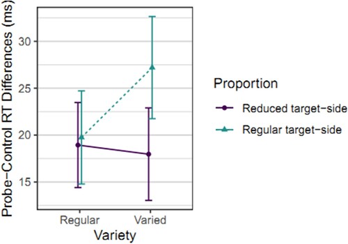
A t-test (using the full sample of 553 participants) showed the Varied filler conditions to have larger probe-control differences than the Regular filler conditions, though with a weak evidence, 3.61 ms, 90% CI [0.96, ∞], t(549.8) = 1.75, p = .041, d = 0.15, 90% CI [0.01, ∞], BF₀₁ = 1.25.

Secondary analysis

A one-sided t-test showed that RT-CITs with arrow symbol nonverbal fillers lead to no larger probe-control differences than those with number string nonverbal fillers, with strong Bayesian evidence, – 3.65 ms, 90% CI [−6.31, ∞] (Mean ± SD = 20.20 ± 24.68 for arrows vs. 23.85 ± 23.92 for numbers), t(542.5) = −1.76, p = .961, d = −0.15, 90% CI [−0.29, ∞], BF₀₁ = 28.20.

Study 3

Given the weak evidence for the increase in probe-control differences when showing a greater variety of target-side fillers, we wanted to replicate this in a third and final study. At the same time, we also wished to examine the flexibility in the choice of filler words and the generalizability of this design to different scenarios (e.g., personal details instead of crime details). This has been repeatedly deliberated ever since the fillers’ introduction (Lukács, Gula, et al., 2017; Wojciechowski & Lukács, 2022). While it has been demonstrated that fillers, specifically importance-related fillers, also enhance the RT-CIT in a crime scenario (Wojciechowski & Lukács, 2022), it is not yet known whether it is beneficial to choose potentially more fitting filler words to each specific scenario or probe. For instance, self-related words are more specifically related to autobiographical details, but generic words related to relevance and recognition could apply to practically any scenario and probe for the RT-CIT. If the former offers no benefit to the latter, always using the same generic words would greatly ease the application and standardisation of the RT-CIT with fillers.

To examine this question, we used a hidden identity scenario (autobiographical details as probes), as this seemed more clearly suitable for the selection of more specific fillers (namely, self-references as opposed to general relevance-references). This also allowed us to indirectly compare our novel findings, regarding the influence of the variations of the RT-CIT, with fillers between the novel mock cybercrime scenario that we used in the first two experiments and the more often used method drawing on the concealment of autobiographical details. As explained earlier, the choice of the exact memory tested might have an impact for a variety of reasons, ranging from the higher relevance of central autobiographical details (as compared to that of the mock crime related information) to the potentially closer correspondence of the mock cybercrime scenario than of the autobiographical memory test to the typical intended use cases outside scientific investigations (e.g., to use the RT-CIT to reveal crime knowledge where suspects try to conceal this knowledge).

Method

Participants

The participants were psychology undergraduate students at the University of Vienna, taking part in exchange for course credits. Collection stopped when the preregistered fixed number of 250 valid participations was reached. Due to changes in the COVID-19 pandemic-related regulations of the University of Vienna's participant pool, the collection was in one phase online (students completing the experiment from home), in another phase offline (at the university’s behavioural laboratory) – however, apart from minor administrative details, the two phases (and in particular the RT-CITs) were identical, using the same website.

We excluded data from two participants who had, within their experimental group, an accuracy rate further than 3 interquartile range (IQR) distance from the lower bound of the IQR, for any of the following item types: (a) nontargets (probe and controls merged), (b) targets, and (c) fillers (all fillers merged). This left the following: Generic condition, 132 subjects (age = 21.6 ± 2.1 [6% unknown]; 33% male, 67% female [1% unknown]; 78% participated online), Specific condition, 118 subjects (age = 21.4 ± 2.1 [4% unknown]; 36% male, 64% female [2% unknown]; 69% participated online).

There were no dropouts among in-laboratory participants; the number of dropouts among online participants was not recorded, but even based on the number of overall site accesses (which includes testing by experiment leaders, etc.), this was not larger than 5% in either group.

Procedure

The procedure was the same as in Study 2, aside from the modifications highlighted in this next section.

Instead of mock crime details, we used autobiographical details as probes: Participants were asked to provide their surname and their birthday (month and day). They were then informed that the following task simulates a lie detection scenario, during which they should try to hide their autobiographical details. They were then presented a list of seven randomly chosen surnames and a list of seven random dates. Neither list contained the given probes (the name or birthday of the given participant), but they had the closest possible character length to the given probe, and none of them started with the same letter. The participants were asked to choose any (but a maximum of two) items in each list that were personally meaningful to them or appeared different in any way from the rest of the items on these lists. Subsequently, five surnames and five dates for the RT-CIT were randomly selected from the non-chosen items (as this assured the neutrality of the controls). One of these items was randomly chosen as the target, while the remaining four served as controls.

There was again one two-level between-subjects factor, and one two-level within-subject factor. For the between-subjects factor “Specificity,” half of all participants had fillers that closely related to the specific probe (expressing primarily self-relatedness, belonging, e.g., “Mine” and “My own”⁷), while the other half of the participants had fillers that generically refer to the recognised relevance of the probe (e.g., “Relevant” and “Recognized”⁸). The within-subject factor “Variety” had the same design as in Study 2, except that in Study 3 it was not between-subjects: One half of the test (first or last two blocks) had three different fillers, while the other half had six different fillers.

There were altogether four blocks (instead of eight, as in Studies 1 and 2), alternating the surname and birthday probe categories and items (with randomly chosen first category). However, each block had the same trial length as two blocks in Studies 1 and 2 (with nontarget fillers included); hence, the overall RT-CIT length was also the same.

Results

Aggregated means of RT means and probe-control differences for the different stimulus types in each condition, are given in Table 5.

Table 5. Reaction time means per condition, in Study 3.

	Generic		Specific
	Regular	Varied	Regular	Varied
Probe	523 ± 55	522 ± 62	513 ± 64	531 ± 68
Control	454 ± 48	457 ± 52	445 ± 60	456 ± 59
Target	565 ± 51	566 ± 52	553 ± 54	566 ± 58
NT-Filler	436 ± 42	438 ± 44	424 ± 55	433 ± 53
T-Filler	557 ± 46	556 ± 46	545 ± 45	560 ± 50
P – C	69.1 ± 33.8	64.9 ± 36.7	68.0 ± 31.3	75.1 ± 36.2
AUCsim	.933	.959	.966	.966

Note: Means and SDs (in the format of M ± SD) for individual reaction time (RT) means; for Probe (incriminating credit card details), Control (other, irrelevant details), Target (the designated control details that require a different response), P – C (individual probe minus control response times). T-Filler = Target filler; NT-Filler = Nontarget filler; AUC_sim: simulated Area Under the Curve.

As preregistered, we examined only the main effects. We obtained moderate evidence for the absence of Filler Type effect, with 1.17 ms, 90% CI [−2.81, ∞], t(491.0) = 0.38, p = .353, d = 0.03, 90% CI [−0.11, ∞], BF₀₁ = 7.28 (one-sided t-test, expecting larger values in the Varied condition)⁹; as well as for the absence of Specificity effect, with only nominally larger probe-control differences for more specific fillers, with 4.40 ms, 95% CI [−2.88, 11.67], t(246.1) = 1.19, p = .235, d = 0.15, 95% CI [−0.10, 0.40], BF₀₁  = 3.69.

Secondary analysis

We conducted planned comparisons to examine order effects on the probe-control RT differences, using one-sided t-tests. First, we compared the within-subject results from the first versus last halves of the tests (i.e., first two vs. last two blocks; test phase effect). As expected (Lukács, 2022), the differences were larger in the first half, by 8.58 ms, 90% CI [5.69, ∞] (Mean ± SD = 73.45 ± 36.59 for first half vs. 64.86 ± 32.23 for second half), t(249) = 3.82, p < .001, d = 0.24, 90% CI [0.14, ∞], BF₁₀ = 156.42. Second, we compared the between-subjects results with Varied condition in first half versus Varied condition in last half (i.e., overall effect of condition order). While, in line with the expectations, the values were nominally somewhat larger in case of Varied condition in the second half, the statistics support neither difference nor equivalence, 3.57, 90% CI [−1.18, ∞] (Mean ± SD = 70.59 ± 29.71 for Varied first vs. 67.03 ± 28.67 for Varied second), t(246.5) = 0.97, p = .168, d = 0.12, 90% CI [−0.09, ∞], BF₀₁ = 2.81. Finally, we repeated test for the Variety effect between-subjects, separately in the first and in the second halves of the tests, again expecting in both cases larger values in the event of more variety in target-side fillers, but neither was significant; first half: 4.50, 90% CI [−1.40, ∞] (Mean ± SD = 75.57 ± 39.33 for Varied vs. 71.07 ± 33.27 for Regular), t(247.3) = 0.98, p = .164, d = 0.12, 90% CI [−0.09, ∞], BF01 = 2.79; second half: −3.11, 90% CI [−8.37, ∞] (Mean ± SD = 63.22 ± 32.60 for Varied vs. 66.33 ± 31.94 for Regular), t(243.7) = −0.76, p = .776, d = −0.10, 90% CI [−0.30, ∞], BF₀₁ = 11.93.

As a final examination of the use of arrows versus numbers, we again compared their respective probe-control RT mean differences in an exploratory way, with a not preregistered t-test, again supporting equivalence, 0.75, 95% CI [−6.53, 8.03] (Mean ± SD = 69.25 ± 30.14 for numbers vs. 68.50 ± 28.22 for arrows), t(244.9) = 0.20, p = .840, d = 0.03, 95% CI [−0.22, 0.27], BF₀₁ = 7.05.

General discussion

In the present study, we have tested novel versions of the RT-CIT with filler items in a new mock cybercrime scenario to study the impact of our manipulations on probe-control RT differences. In general, we found that the RT-CIT, though showing apparently modest diagnostic accuracy (as not unusual for mock crimes in general), does work (i.e., produces statistically significant probe-control RT differences) in the mock cybercrime scenario. However, we did not find significant improvements of the novel versions over the original version. All our conclusions were based on well-powered tests, as indicated by generally narrow CIs as well as, in most cases, substantial Bayesian evidence that also allowed several demonstrations of practical equivalence.

In Study 1, we showed that (a) the inclusion of nontarget fillers is important for the RT-CIT effect (i.e., higher probe-control RT differences), and (b) whether nontarget fillers are words with meaningful relations to the nontarget semantics or nonverbal items without meaningful relations to the nontarget semantics has no substantial influence. Since using nonverbal nontarget fillers was shown non-inferior to verbal ones, one may construct tests using nonverbal items to facilitate practical implementation (i.e., without the need for selecting and optimising six specific ideal nontarget filler words). We have used two different types of nonverbal fillers: arrow symbols and number strings. In each of the three experiments, we have demonstrated their equivalence. Therefore, for easier and more straightforward practical implementation, we recommend the use of number strings (since arrow symbols might differ across different operating systems and software, or may not even be available, especially in the context of web-based implementations).

In Study 2, we manipulated the proportion (overall frequency) of target-side items (targets and target-side fillers), as well as the variety of target-side fillers (the number of different filler words employed, regardless of the overall number of filler trials). For the proportion manipulation, we reduced the conventional numbers (18 targets and 18 target-side fillers for each block of 126 other items: 18 probes, 72 controls, and 36 nontarget fillers) to about half (10 targets and 10 target-side fillers for each block of 126 other items). We found that the reduced proportion of target-side items either decreased or did not substantially affect probe-control differences, depending on filler variety (see below).

Regarding variety, we found that a greater variety of (target-side) fillers may have increased probe-control differences. However, the evidence for this difference was weak, and therefore, we replicated this in Study 3 with a more conventional design using central autobiographical detail, where we instead found substantial evidence for equivalence. As already previously suggested (Lukács & Ansorge, 2021, p. 2821), there might be a level of sufficient complexity implied by using fillers and including more fillers may not elicit further effect or even be detrimental instead. Some potential support for this is the interaction between filler variety and the proportion of target-side fillers: Variety led to substantial enhancement only in case of the conventional proportion of target-side items, but not in case of reduced proportion (Figure 4).

This altogether could be tentatively interpreted as follows. First, reduced target-side items increases the salience of the semantic dimension, fostering the probe-control difference (as proposed in the introduction to Study 2), but the benefit of this salience is offset by the detriment due the concomitant decrease of attention to target-side items: With so few items in the task, participants may pay less attention to each of them and be more inclined to resort to the default nontarget category or response (i.e., the response that is required for the large proportion of items), masking probe-control differences. The assumption is supported by the generally faster RTs (Table 4) and lower accuracies (see online Appendix) for nontarget items. Second, the variety introduced in case of reduced proportion further complicates target-side responses by the difficulty of remembering and recognising all the different items, and therefore, participants are even more inclined to default to nontarget responses. (Again, faster RTs and lower accuracies in this specific combination seem to support this assumption.)

In Study 3, apart from the failed replication of the effect of variety, we tested whether the RT-CIT may be more efficient if the (target-side) fillers do not generically refer to relevance, but more specifically to the items included in the test (here: autobiographical items, hence using self-referring target-side fillers). We found no evidence for any difference, but instead moderate evidence for equivalence. This indicates that, while it is important that fillers in some way refer to the probe item (as repeatedly demonstrated by Lukács & Ansorge, 2021), the strict probe-relatedness of the filler plays no major role, and it may be that one can either choose filler words fairly liberally in any given context (cf. Koller et al., 2022) or quite simply always use a set of generic relevance-referring filler words as in our study (and as may be optimised in the future for each given language).

Lastly, regarding our cybercrime scenario, while the salience of items has been repeatedly shown to influence results, the relevance and robustness of this issue is again highlighted by the striking difference in the present case (e.g., AUC estimates around .70 for crime details, and around .95 for autobiographical items, despite otherwise near-identical RT-CIT designs). Given the freely available source code, the cybercrime scenario could be reused in any future RT-CIT study as, at the very least, a fair substitute for offline enactments of a mock crime. However, we would also recommend further studies investigating if the diminution of the mock cybercrime scenario is due to the lower general everyday relevance of the information in this scenario than of central autobiographical detail or if it may be due to some specific side condition of this crime-related scenario (e.g., the conviction of the participants that prosecution is less likely in these cases, implying less proactive suppression during concealment).

At the outset, we have argued that the probe-control differences in RT-CITs are probably reflective of response conflicts based on the participants’ tendency to misclassify semantically salient probes as targets (cf. Seymour & Schumacher, 2009). However, it is possible that, more generally, the implied negation of one’s knowledge of the probes accounted for some of the response delays to the probes too (e.g., Foerster et al., 2017). In either case, one can try to compare the presently found effects to that reported in the literature. The present effect sizes of the probe-control differences ranged between 9.1 ms (d = 0.39) in Study 1 and 75.1 ms (d = 2.07) in Study 3, depending on side conditions, such as whether the probes corresponded to information relevant only for a relatively short time (Study 1) or to relevant, long-term memory content (Study 3). The effects found are therefore comparable to those reported in the literature on related effects, such as category-priming effects (e.g., Lucas, 2000) or lying-elicited response delays (cf. Suchotzki et al., 2017). In addition, like these priming and lying effects, the net probe-control differences are likely not only reflective of the underlying difficulty of resolving response conflict and/or lying (i.e., negating one’s knowledge), but also of the occasional successful (proactive) suppression of the automatic processing of the probe’s “true” meaning (cf., Experiment 2 of Kinoshita et al., 2011). Thus, in the future, further measures of suppression (e.g., physiological) could be tested for their potential to identify and filter out trials in which participants successfully and proactively suppressed the probe’s meaning, and thereby increase probe-control differences and RT-CIT sensitivity.

In a supplementary analysis (in the Appendix), we also revealed substantial task-switching effects in the RT-CIT. This finding underlines the importance of properly balanced stimulus order.

Conclusion

Regarding fillers in the RT-CIT, we have two main conclusions. First, the fillers are largely optimal as they were originally introduced (Lukács, Kleinberg, et al., 2017), although one may replace verbal nontarget fillers with nonverbal items for easier implementation in a variety of languages and scenarios. Second, the target fillers seem robust to specific choices of words, and one does not need to customise them to each new use case, but may use generic ones (related to relevance, recognition) in all scenarios. Taken together, for future RT-CITs, we recommend the use of generic recognition-referring target fillers and nonverbal nontarget fillers. We have also demonstrated that the RT-CIT is viable in a cybercrime scenario. However, the relatively low effects and diagnostic accuracies reemphasize the importance of assessments in realistic scenarios as well as the need for further improving the RT-CIT.

Acknowledgements

We thank Claudia “Kiki” Kawai for her informal contributions to the original concepts of our studies and for kindly proofreading the manuscript. We thank Till Lubczyk for testing the online crime scenario and his very helpful related suggestions. Finally, thanks to Sabrina Ebel, Tobias Greif, and Lea Bachmann for assisting with the (in-lab) data collection. Authors’ Contributions: Concept, study design, software, and analysis by G. L.; manuscript by G. L. and U. A.

Disclosure statement

No potential conflict of interest was reported by the author(s).

Data availability statement

Codes for the experiment websites, all collected data, and analysis scripts are available [temporarily masked for review] via https://osf.io/a4q5n/?view_only=6754a8fd9c22487989fc94ac4878fe02.

Notes

1 For demo purposes, the server connection was removed, all items are available on the user-side, and all input (e.g., bank name or PIN) is accepted as “correct” except those with invalid character lengths.

2 We could have also used any free email service, but we assumed that an official email account would increase the realism of the crime.

3 The same names were used as by Seymour et al. (2000).

4 The lists of all items (for both infiltrated email accounts) used in the RT-CIT are available via the OSF repository.

5 The randomization happened in such double-blocks because the number of items within a single block would not have allowed preceding each item exactly one time. Regarding the importance of preceding trial types, please see the Appendix.

6 The data with arrows did not closely follow normal distribution (Shapiro-Wilk test: W = 0.84, p < .001), so we also performed rank tests: The median was lower when using arrows, with an estimate of –1.40 ms, 95% CI [–6.39, 3.64] (Median ± MAD = 11.76 ± 18.99 vs. 14.01 ± 16.27), but the test again indicated equivalence, U = 5155.00, p = .589, d = 0.05, 95% CI [–0.22, 0.32], BF₀₁ = 6.62 (van Doorn et al., 2020).

7 The full list is: “Mein” (mine), “Eigene” (own), “Selbst” (self), “Persönlich” (personal), “Zugehörig” (related/associated, such as with a person), and, depending on category, “Mein Name” (my name), or “Geburtstag” (birthday).

8 The full list is: “Relevant” (relevant), “Erkannt” (recognised), “Bedeutsam” (meaningful/significant), “Entdeckt” (detected/recognised), “Wesentlich” (vital/significant), and, chosen randomly, “Wichtig” (important), or “Essenziell” (essential).

9 The Varied condition’s values did not closely follow normal distribution (Shapiro-Wilk test: W = 0.98, p = .005), so we also performed rank tests, but the results were very similar, with an estimate of 0.79 ms, 90% CI [–3.18, ∞] (Median ± MAD = 65.42 ± 30.62 vs. 65.60 ± 35.06), U = 31667.00, p = .398, BF₀₁ = 8.06.

Appendix

The importance of preceding trials: task-switching effects in the RT-CIT

Here, we demonstrate that the order of items impacts the outcome via task-switching effects (e.g., Klauer & Mierke, 2005). This is based on the assumption that the probes are erroneously categorised together with the targets, such that preceding controls or nontarget fillers prior to probe trials would correspond to a change of the task set. (Note, though, that no corresponding substantial effect is present with the controls.) We collected data from 593 valid individual tests (all on “guilty” participants, i.e., ones recognising the relevant probe) using RT-CIT with fillers, from seven different previous experiments (Lukács, 2021a; Exp. 1, 2; and 4 from Lukács et al., 2021; Exp. 1 from Lukács, Kleinberg, et al., 2017; Exp. 2 from Lukács & Ansorge, 2019; and one yet unpublished experiment). In Figure A1, we present the RT differences per item type that precedes the upcoming item (all data and analysis scripts, as well as supplementary figures, are available via the OSF repository). The patterns of differences are consistent across different experiments, and statistically robust, with p < .001 for all relevant comparisons (between probe RTs and probe-control RT differences).

Figure A1. Response times per item type and per preceding item type.

Note: Response times per item type and per preceding item type. Aggregated reaction times (RTs) in ms (on the y axis) from all individual tests. The missing data point for probes preceding probes is because this never occurs when the item order is well balanced, given that the probes are infrequent items in the RT-CIT. T-filler: target-side filler; NonT-filler: nontarget-side filler.

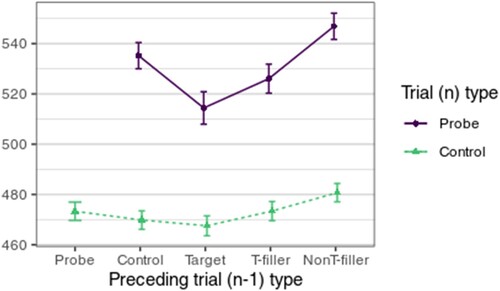
Given that innocent results tend to range between ca. – 20 and 20 ms, with decision criteria often placed at around 20 ms (Lukács & Specker, 2020; Noordraven & Verschuere, 2013), the differences of 30 ms, the apparent magnitude of task-switching effect in some cases (Figure A1), mean a vast potential bias in individual tests. Therefore, for correct individual classifications, it is crucial to properly balance item order.

References

- Anderson, R., Barton, C., Böhme, R., Clayton, R., van Eeten, M. J. G., Levi, M., Moore, T., & Savage, S. (2013). Measuring the cost of cybercrime. In R. Böhme (Ed.), The economics of information security and privacy (pp. 265–300). Springer. https://doi.org/10.1007/978-3-642-39498-0_12
- Broadhead, S. (2018). The contemporary cybercrime ecosystem: A multi-disciplinary overview of the state of affairs and developments. Computer Law & Security Review, 34(6), 1180–1196. https://doi.org/10.1016/j.clsr.2018.08.005
- Delacre, M., Lakens, D., & Leys, C. (2017). Why psychologists should by default use Welch’s t-test instead of student’s t-test. International Review of Social Psychology, 30(1), 92–101. https://doi.org/10.5334/irsp.82
- Elaad, E., Ginton, A., & Jungman, N. (1992). Detection measures in real-life criminal guilty knowledge tests. Journal of Applied Psychology, 77(5), 757–767. https://doi.org/10.1037/0021-9010.77.5.757
- Eom, J.-S., Sohn, S., Park, K., Eum, Y.-J., & Sohn, J.-H. (2016). Effects of varying numbers of probes on RT-based CIT accuracy. International Journal of Multimedia and Ubiquitous Engineering, 11(2), 229–238. https://doi.org/10.14257/ijmue.2016.11.2.23
- Fawcett, T. (2006). An introduction to ROC analysis. Pattern Recognition Letters, 27(8), 861–874. https://doi.org/10.1016/j.patrec.2005.10.010
- Foerster, A., Wirth, R., Herbort, O., Kunde, W., & Pfister, R. (2017). Lying upside-down: Alibis reverse cognitive burdens of dishonesty. Journal of Experimental Psychology: Applied, 23(3), 301–319. https://doi.org/10.1037/xap0000129
- Green, D. M., & Swets, J. A. (1974). Signal detection theory and psychophysics. R. E. Krieger Pub. Co.
- Greenwald, A. G., McGhee, D. E., & Schwartz, J. L. (1998). Measuring individual differences in implicit cognition: The implicit association test. Journal of Personality and Social Psychology, 74(6), 1464–1480. https://doi.org/10.1037/0022-3514.74.6.1464
- Hartwig, M., & Bond, C. F. (2011). Why do lie-catchers fail? A lens model meta-analysis of human lie judgments. Psychological Bulletin, 137(4), 643–659. https://doi.org/10.1037/a0023589
- Hu, X., Evans, A., Wu, H., Lee, K., & Fu, G. (2013). An interfering dot-probe task facilitates the detection of mock crime memory in a reaction time (RT)-based concealed information test. Acta Psychologica, 142(2), 278–285. https://doi.org/10.1016/j.actpsy.2012.12.006
- Jarosz, A. F., & Wiley, J. (2014). What are the odds? A practical guide to computing and reporting Bayes factors. The Journal of Problem Solving, 7(1), 2–9. https://doi.org/10.7771/1932-6246.1167
- Jeffreys, H. (1961). Theory of probability (3rd ed.). Oxford University Press.
- Kelley, K. (2019). MBESS: The MBESS R package. R package version 4.5.1. https://CRAN.R-project.org/package=MBESS
- Kinoshita, S., Mozer, M. C., & Forster, K. I. (2011). Dynamic adaptation to history of trial difficulty explains the effect of congruency proportion on masked priming. Journal of Experimental Psychology: General, 140(4), 622–636. http://doi.org/10.1037/a0024230
- Klauer, K. C., & Mierke, J. (2005). Task-set inertia, attitude accessibility, and compatibility-order effects: New evidence for a task-set switching account of the implicit association test effect. Personality and Social Psychology Bulletin, 31(2), 208–217. https://doi.org/10.1177/0146167204271416
- Kleinberg, B., & Verschuere, B. (2015). Memory detection 2.0: The first web-based memory detection test. Plos One, 10(4), e0118715. https://doi.org/10.1371/journal.pone.0118715
- Koller, D., Hofer, F., Ghelfi, S., & Verschuere, B. (2022). Nationality check in the face of information contamination: Testing the inducer-CIT and the autobiographical IAT. Psychology, Crime & Law, 1–20. https://doi.org/10.1080/1068316X.2022.2102170
- Lakens, D. (2013). Calculating and reporting effect sizes to facilitate cumulative science: A practical primer for t-tests and ANOVAs. Frontiers in Psychology, 4, Article 863. https://doi.org/10.3389/fpsyg.2013.00863
- Lakens, D., Scheel, A. M., & Isager, P. M. (2018). Equivalence testing for psychological research: A tutorial. Advances in Methods and Practices in Psychological Science, 1(2), 259–269. https://doi.org/10.1177/2515245918770963
- Lawrence, M. A. (2016). Ez: Easy analysis and visualization of factorial experiments. R package version 4.4-0. https://CRAN.R-project.org/package=ez
- Lieblich, I., Naftali, G., Shmueli, J., & Kugelmass, S. (1974). Efficiency of GSR detection of information with repeated presentation of series of stimuli in two motivational states. Journal of Applied Psychology, 59(1), 113–115. https://doi.org/10.1037/h0035781
- Lord, F. M., & Novick, M. R. (2008). Statistical theories of mental test scores. Information Age Publishing Inc.
- Lucas, M. (2000). Semantic priming without association: A meta-analytic review. Psychonomic Bulletin & Review, 7(4), 618–630. https://doi.org/10.3758/BF03212999
- Lukács, G. (2021a). Addressing selective attrition in the enhanced response time-based concealed information test: A within-subject replication. Applied Cognitive Psychology, 35(1), 243–250. https://doi.org/10.1002/acp.3759
- Lukács, G. (2021b). Neatstats: An R package for a neat pipeline from raw data to reportable statistics in psychological science. The Quantitative Methods for Psychology, 17(1), 7–23. https://doi.org/10.20982/tqmp.17.1.p007
- Lukács, G. (2022). Prolonged response time concealed information test decreases probe-control differences but increases classification accuracy. Journal of Applied Research in Memory and Cognition, 11(2), 188–199. https://doi.org/10.1016/j.jarmac.2021.08.008
- Lukács, G., & Ansorge, U. (2019). Information leakage in the response time-based concealed information test. Applied Cognitive Psychology, 33(6), 1178–1196. https://doi.org/10.1002/acp.3565
- Lukács, G., & Ansorge, U. (2021). The mechanism of filler items in the response time concealed information test. Psychological Research, 85(7), 2808–2828. https://doi.org/10.1007/s00426-020-01432-y
- Lukács, G., Gula, B., Szegedi-Hallgató, E., & Csifcsák, G. (2017). Association-based concealed information test: A novel reaction time-based deception detection method. Journal of Applied Research in Memory and Cognition, 6(3), 283–294. https://doi.org/10.1016/j.jarmac.2017.06.001
- Lukács, G., Kawai, C., Ansorge, U., & Fekete, A. (2021). Detecting concealed language knowledge via response times. Applied Linguistics Review, https://doi.org/10.1515/applirev-2020-0130
- Lukács, G., Kleinberg, B., Kunzi, M., & Ansorge, U. (2020). Response time concealed information test on smartphones. Collabra: Psychology, 6(1), Article 4. https://doi.org/10.1525/collabra.255
- Lukács, G., Kleinberg, B., & Verschuere, B. (2017). Familiarity-related fillers improve the validity of reaction time-based memory detection. Journal of Applied Research in Memory and Cognition, 6(3), 295–305. https://doi.org/10.1016/j.jarmac.2017.01.013
- Lukács, G., & Specker, E. (2020). Dispersion matters: Diagnostics and control data computer simulation in concealed information test studies. Plos One, 15(10), e0240259. https://doi.org/10.1371/journal.pone.0240259
- Makowski, D., Ben-Shachar, M., & Lüdecke, D. (2019). Bayestestr: Describing effects and their uncertainty, existence and significance within the Bayesian framework. Journal of Open Source Software, 4(40), 1541. https://doi.org/10.21105/joss.01541
- Matsuda, I., Nittono, H., & Ogawa, T. (2013). Identifying concealment-related responses in the concealed information test. Psychophysiology, 50(7), 617–626. https://doi.org/10.1111/psyp.12046
- Meijer, E. H., klein Selle, N., Elber, L., & Ben-Shakhar, G. (2014). Memory detection with the concealed information test: A meta analysis of skin conductance, respiration, heart rate, and P300 data. Psychophysiology, 51(9), 879–904. https://doi.org/10.1111/psyp.12239
- Meijer, E. H., Verschuere, B., Gamer, M., Merckelbach, H., & Ben-Shakhar, G. (2016). Deception detection with behavioral, autonomic, and neural measures: Conceptual and methodological considerations that warrant modesty. Psychophysiology, 53(5), 593–604. https://doi.org/10.1111/psyp.12609
- Meixner, J. B., & Rosenfeld, J. P. (2014). Detecting knowledge of incidentally acquired, real-world memories using a P300-based concealed-information test. Psychological Science, 25(11), 1994–2005. https://doi.org/10.1177/0956797614547278
- Morey, R. D., & Rouder, J. N. (2018). BayesFactor: Computation of Bayes factors for common designs. R package version 0.9.12-4.2. https://CRAN.R-project.org/package=BayesFactor
- National Research Council. (2003). Polygraph and lie detection. The National Academies Press. http://www.nap.edu/openbook.php?record_id=10420
- Noordraven, E., & Verschuere, B. (2013). Predicting the sensitivity of the reaction time-based concealed information test. Applied Cognitive Psychology, 27(3), 328–335. https://doi.org/10.1002/acp.2910
- Norman, D. G., Gunnell, D. A., Mrowiec, A. J., & Watson, D. G. (2020). Seen this scene? Scene recognition in the reaction-time concealed information test. Memory & Cognition, 48(8), 1388–1402. https://doi.org/10.3758/s13421-020-01063-z
- Olson, J., Rosenfeld, J. P., & Perrault, E. (2020). Familiarity-related filler items enhance the RT CIT, but not the P300 CIT: Episodic vs. Semantic memory protocols. International Journal of Psychophysiology, 158, 370–379. https://doi.org/10.1016/j.ijpsycho.2020.10.001
- Osugi, A. (2011). Daily application of the concealed information test: Japan. In B. Verschuere, G. Ben-Shakhar, & E. Meijer (Eds.), Memory detection (pp. 253–275). Cambridge University Press. https://doi.org/10.1017/CBO9780511975196.015
- Peth, J., Vossel, G., & Gamer, M. (2012). Emotional arousal modulates the encoding of crime-related details and corresponding physiological responses in the concealed information test. Psychophysiology, 49(3), 381–390. https://doi.org/10.1111/j.1469-8986.2011.01313.x
- R Core Team. (2020). R: A language and environment for statistical computing. R Foundation for Statistical Computing. https://www.R-project.org/
- Rosenfeld, J. P., Biroschak, J. R., & Furedy, J. J. (2006). P300-based detection of concealed autobiographical versus incidentally acquired information in target and non-target paradigms. International Journal of Psychophysiology, 60(3), 251–259. https://doi.org/10.1016/j.ijpsycho.2005.06.002
- Rothermund, K., & Wentura, D. (2004). Underlying processes in the implicit association test: Dissociating salience from associations. Journal of Experimental Psychology: General, 133(2), 139–165. https://doi.org/10.1037/0096-3445.133.2.139
- Seymour, T. L., & Schumacher, E. H. (2009). Electromyographic evidence for response conflict in the exclude recognition task. Cognitive, Affective, & Behavioral Neuroscience, 9(1), 71–82. https://doi.org/10.3758/CABN.9.1.71
- Seymour, T. L., Seifert, C. M., Shafto, M. G., & Mosmann, A. L. (2000). Using response time measures to assess "guilty knowledge".. Journal of Applied Psychology, 85(1), 30–37. https://doi.org/10.1037/0021-9010.85.1.30
- Smith, R., Grabosky, P., & Urbas, G. (2004). Cyber criminals on trial. Criminal Justice Matters, 58(1), 22–23. https://doi.org/10.1080/09627250408553240
- Suchotzki, K., De Houwer, J., Kleinberg, B., & Verschuere, B. (2018). Using more different and more familiar targets improves the detection of concealed information. Acta Psychologica, 185, 65–71. https://doi.org/10.1016/j.actpsy.2018.01.010
- Suchotzki, K., Verschuere, B., & Gamer, M. (2021). How vulnerable is the reaction time concealed information test to faking? Journal of Applied Research in Memory and Cognition, 10(2), 268–277. https://doi.org/10.1016/j.jarmac.2020.10.003
- Suchotzki, K., Verschuere, B., Peth, J., Crombez, G., & Gamer, M. (2015). Manipulating item proportion and deception reveals crucial dissociation between behavioral, autonomic, and neural indices of concealed information. Human Brain Mapping, 36(2), 427–439. https://doi.org/10.1002/hbm.22637
- Suchotzki, K., Verschuere, B., Van Bockstaele, B., Ben-Shakhar, G., & Crombez, G. (2017). Lying takes time: A meta-analysis on reaction time measures of deception. Psychological Bulletin, 143(4), 428–453. https://doi.org/10.1037/bul0000087
- Swanson, C. L., James, L. E., & Ingram, R. E. (2021). Incidental learning of proper names and “earwitness” recall. Memory, 29(5), 637–644. https://doi.org/10.1080/09658211.2021.1925301
- van Doorn, J., Ly, A., Marsman, M., & Wagenmakers, E.-J. (2020). Bayesian rank-based hypothesis testing for the rank sum test, the signed rank test, and Spearman’s ρ. Journal of Applied Statistics, 1–23. https://doi.org/10.1080/02664763.2019.1709053
- Verschuere, B., & De Houwer, J. (2011). Detecting concealed information in less than a second: Response latency-based measures. In B. Verschuere, G. Ben-Shakhar, & E. Meijer (Eds.), Memory detection (pp. 46–62). Cambridge University Press. https://doi.org/10.1017/CBO9780511975196.004
- Verschuere, B., Kleinberg, B., & Theocharidou, K. (2015). RT-based memory detection: Item saliency effects in the single-probe and the multiple-probe protocol. Journal of Applied Research in Memory and Cognition, 4(1), 59–65. https://doi.org/10.1016/j.jarmac.2015.01.001
- Visu-Petra, G., Varga, M., Miclea, M., & Visu-Petra, L. (2013). When interference helps: Increasing executive load to facilitate deception detection in the concealed information test. Frontiers in Psychology, 4, Article 146. https://doi.org/10.3389/fpsyg.2013.00146
- Wagenmakers, E. J. (2007). A practical solution to the pervasive problems of p values. Psychonomic Bulletin & Review, 14(5), 779–804. https://doi.org/10.3758/BF03194105
- Wickham, H. (2016). Ggplot2: Elegant graphics for data analysis (2nd ed.). Springer.
- Wojciechowski, J., & Lukács, G. (2022). Importance-related fillers improve the classification accuracy of the response time concealed information test in a crime scenario. Legal and Criminological Psychology, 27(1), 82–100. https://doi.org/10.1111/lcrp.12198
- Zhou, H., & Fishbach, A. (2016). The pitfall of experimenting on the web: How unattended selective attrition leads to surprising (yet false) research conclusions. Journal of Personality and Social Psychology, 111(4), 493–504. https://doi.org/10.1037/pspa0000056