Broadcast domination of lexicographic and modular products of graphs

Abstract

A dominating broadcast labeling of a graph G is a function $f:V(G)\to \{0,1,2,\dots ,\mathit{diam}(G)\}$ such that $f(v)\le e(v)$ for all $v\in V(G),$ where e(v) is the eccentricity of v, and for every vertex $u\in V(G),$ there exists a vertex v with $f(v)\ge 1$ and $d(u,v)\le f(v).$ The cost of f is $\sum _{v\in V(G)}f(v).$ The minimum of costs over all the dominating broadcast labelings of G is called the broadcast domination number ${\gamma }_b(G)$ of G. In this paper, we give bounds to the broadcast domination number of lexicographic product G • H of a connected graph G and a graph H, and we show that the bounds are tight by determining the exact values for lexicographic products of some classes of graphs. Also, we give an algorithm which produces a dominating broadcast labeling of G • H. We use the algorithm to find ${\gamma }_b(P_m$ • $H)$ and ${\gamma }_b(C_m$ • $H).$ Further, we give an upper bound for the broadcast domination number of the modular product of two connected graphs and exact values are determined for the modular product of two graphs involving path, cycle and complete graphs.

Keywords:

• Dominating broadcast labeling
• broadcast domination number
• lexicographic product
• modular product

2010 MATHEMATICS SUBJECT CLASSIFICATION::

• 05C69
• 05C76
• 05C78

1. Introduction

A radio station wishes to install broadcasting towers of varying capacities in different sections/locations of a region so that the whole region can hear their broadcast. A broadcasting tower of larger capacity broadcasts further but attracts more cost. So, it is an obvious target to install towers, tactically, of appropriate capacities in order to minimize the total cost. This lead to the concept of broadcast domination in a graph. The situation was modeled as a graph whose vertices are different sections/locations of the region and two vertices are adjacent if those two corresponding sections/locations are close enough. Erwin [4] has introduced the concept of broadcast domination.

A broadcast labeling of a graph G is a function $f:V(G)\to \{0,1,2,\dots ,\mathit{diam}(G)\}$ such that $f(v)\le e(v)$ for all v $\in$ V(G), where e(v) is the eccentricity of v. The cost of f is $\sum _{v\in V(G)}f(v)$ and is denoted by $\sigma (f).$ A vertex v is a broadcast vertex if $f(v)\ge 1$ and the set of all broadcast vertices is denoted by $V_f^{+}(G)$ or simply $V_f^{+}.$ A vertex $u\in V(G)$ is said to be f-dominated if there exists a vertex $v\in V_f^{+}$ such that $d(u,v)\le f(v).$ It is clear that a broadcast vertex f-dominates itself. For each vertex $v\in V_f^{+},$ the closed f-neighborhood $N_f[v]$ of v is the set $\{u\in V(G):d(u,v)\le f(v)\}.$ A broadcast labeling f is said to be a dominating broadcast labeling if $\underset{v\in V_f^{+}}{\cup }{N}_f[v]=V(G)$ and the broadcast domination number ${\gamma }_b(G)$ of G is defined as $\min \{\sigma (f):fisa\mathit{dominating}\mathit{broadcast}\mathit{labeling}ofG\}.$ A dominating broadcast labeling f is said to be an optimal dominating broadcast labeling if $\sigma (f)={\gamma }_b(G).$ A dominating broadcast labeling f is said to be an efficient dominating broadcast labeling if every vertex is f-dominated by exactly one broadcast vertex. From now onwards, we use DBL and ODBL in place of dominating broadcast labeling and optimal dominating broadcast labeling, respectively.

For any two graphs G and H, there are four standard graph products, namely, Cartesian product $G\square H,$ direct product G × H, strong product $G⊠H$ and lexicographic product G • H. The vertex set of each of the products is $V(G)\times V(H)$ and the edge sets are defined as follows.

1. $(u,v)(u^{\prime },v^{\prime })\in E(G\square H)$ if $u{u}^{\prime }\in E(G)$ and $v=v^{\prime },$ or $u=u^{\prime }$ and $v{v}^{\prime }\in E(H).$

2. $(u,v)(u^{\prime },v^{\prime })\in E(G\times H)$ if $u{u}^{\prime }\in E(G)$ and $v{v}^{\prime }\in E(H).$

3. $E(G⊠H)=E(G\square H)\cup E(G\times H).$

4. $(u,v)(u^{\prime },v^{\prime })\in E(G$ • $H)$ if $u{u}^{\prime }\in E(G),$ or $u=u^{\prime }$ and $v{v}^{\prime }\in E(H).$

The broadcast domination for the first three products is studied in [1, 3, 7, 10, 11]. In this paper, we explore the broadcast domination of the lexicographic product and the modular product, where the latter one is closely related to the standard products. 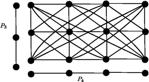For the modular product $G\diamond H$ of G and H, the vertex set is $V(G)\times V(H)$ and the edge set $E(G\diamond H)=E(G\square H)\cup E(G\times H)\cup E(\overline{G}\times \overline{H}).$ The lexicographic product and the modular product of P₃ and P₄ are given in Figures 1 and 2, respectively. It is evident that, among all the mentioned products, only the lexicographic product is non-commutative.

Figure 1. Lexicographic product of P₃ and P₄.

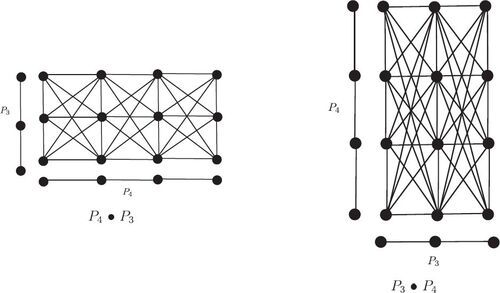
Figure 2. Modular product of P₃ and P_4.

1.1. Literature survey

Erwin [4] has given tight bounds for the broadcast domination number of any graph.

Theorem 1.1

([4]). For a non-trivial connected graph G, $\lceil \frac{\mathit{diam}(G)+1}{3}\rceil \le {\gamma }_b(G)\le \min \{\mathit{rad}(G),\gamma (G)\}.$

Dunbar et al. [3] have proved that every graph has an efficient ODBL. So, whenever required, we consider an efficient ODBL without citing the theorem below.

Theorem 1.2

([3]). Every graph G has an efficient optimal dominating broadcast labeling.

In light of the upper bound given in Theorem 1.1, Dunbar et al. [3] have proposed the following classification of graphs and the relevant studies can be found in [2, 4–6, 8, 9]. A graph G is said to be Type I or radial graph (Type II or 1-cap graph) if ${\gamma }_b(G)=\mathit{rad}(G)$ (${\gamma }_b(G)=\gamma (G)$). If ${\gamma }_b(G)<\min \{\mathit{rad}(G),\gamma (G)\},$ then G is a Type III graph.

Erwin [4] has shown that ${\gamma }_b(P_n)=\lceil \frac{n}{3}\rceil ={\gamma }_b(C_n).$ Brešar and Špacapan [1] have given sharp upper bounds for the broadcast domination numbers of $G\square H,G⊠H$ and G × H, for any two connected graphs G and H, in terms of ${\gamma }_b(G)$ and ${\gamma }_b(H).$ The broadcast domination numbers of some products of graphs involving $P_n,C_n,K_n$ and $K_{1,n}$ are given in [3, 7, 10, 11].

Theorem 1.3

([1]). For any two connected graphs G and H, $$\begin{array}{ccc}{\gamma }_b(G\square H)\hfill & \le \hfill & \frac{3}{2}({\gamma }_b(G)+{\gamma }_b(H)).\hfill \\ {\gamma }_b(G⊠H)\hfill & \le \hfill & \frac{3}{2}\max \{{\gamma }_b(G),{\gamma }_b(H)\}.\hfill \\ {\gamma }_b(G\times H)\hfill & \le \hfill & \{\begin{array}{cc}3\max \{{\gamma }_b(G),{\gamma }_b(H)\}\hfill & if\mathit{rad}(G)\ne \mathit{rad}(H),\hfill \\ 3\max \{{\gamma }_b(G),{\gamma }_b(H)\}+1\hfill & if\mathit{rad}(G)=\mathit{rad}(H).\hfill \end{array}\hfill \end{array}$$

Theorem 1.4

([3]). For any pair of integers $m\ge 2$ and $n\ge 2,{\gamma }_b(P_m\square P_n)=\mathit{rad}(P_m\square P_n)=\lfloor \frac{m}{2}\rfloor +\lfloor \frac{n}{2}\rfloor .$

Theorem 1.5

([11]). For paths P_m and P_n, $$\begin{array}{c}{\gamma }_b(P_m⊠P_n)=\lceil \frac{1}{2}\left(m-\lfloor \frac{m}{\max \{p,3\}}\rfloor \right)\rceil ,\mathit{where}p=2\lceil \frac{n-1}{2}\rceil +1.\hfill \\ {\gamma }_b(P_m\times P_n)=\{\begin{array}{cc}m\hfill & ifn=1,\hfill \\ n\left(\frac{m+1}{n+1}\right)\hfill & ifn⩾2,m,n\mathit{both}\mathit{odd}\mathit{with}\frac{m+1}{n+1}\mathit{integer},\hfill \\ 2\lceil \frac{m-\lfloor \frac{m}{n+1}\rfloor }{2}\rceil \hfill & \mathit{otherwise}.\hfill \end{array}\hfill \end{array}$$ $$\begin{array}{c}{\gamma }_b(P_m•{\mathrm{P}}_{\mathrm{n}})=\{\begin{array}{cc}\max \{\lceil \frac{m}{3}\rceil ,\lceil \frac{n}{3}\rceil \}\hfill & ifm=1orn\in \{1,2,3\},\hfill \\ \max \{\lceil \frac{2m}{5}\rceil ,2\}\hfill & ifm⩾2\mathit{and}n⩾4.\hfill \end{array}\hfill \end{array}$$

Theorem 1.6

([7]). For any two positive integers $m⩾3$ and $n⩾3,$ $$\begin{array}{c}{\gamma }_b(P_m\square K_{1,n})={\gamma }_b(C_m\square K_{1,n})={\gamma }_b(P_m\square K_n)={\gamma }_b(C_m\square K_n)=\lceil \frac{m+1}{2}\rceil and\hfill \\ {\gamma }_b(C_m\square P_n)=\{\begin{array}{cc}\frac{m}{2}\hfill & ifn=2\mathit{and}mis\mathit{even},\hfill \\ \lceil \frac{m}{2}\rceil +\lceil \frac{n}{2}\rceil \hfill & \mathit{otherwise}.\hfill \end{array}\hfill \end{array}$$

Theorem 1.7

([10]). For any two positive integers $m⩾3$ and $n⩾3,{\gamma }_b(C_m\square C_n)=\lceil \frac{m+n}{2}\rceil -1.$

In this paper, first, we give upper and lower bounds to the broadcast domination number of lexicographic product G • H of a connected graph G and a graph H, in terms of ${\gamma }_b(G).$ We find ${\gamma }_b(C_m$ • $K_n),{\gamma }_b(P_m$ • $K_n),{\gamma }_b(K_n$ • $C_m),{\gamma }_b(K_n$ • $P_m)$ and ${\gamma }_b(G$ • $H),$ where G is either a hypercube graph or radial graph and H is any graph with ${\gamma }_b(H)\ge 2.$ We show that these graphs attain either the lower or the upper bound. Further, we give an algorithm which produces a DBL of G • H. We give a lower bound for ${\gamma }_b(P_m$ • $H)$ and ${\gamma }_b(C_m$ • $H),$ and prove that the DBL produced by the algorithm achieves the lower bound. Later, we show that ${\gamma }_b(G\diamond H)$ is at most 3 for any two connected non-complete graphs G and H, and prove that ${\gamma }_b(K_m\diamond H)={\gamma }_b(H).$ Also, we determine the exact values of the broadcast domination numbers of the modular products of graphs involving P_n, C_n and K_n. All the graphs considered in this article are simple and non-trivial.

2. Lexicographic product

We denote the vertex $(u_i,v_j)$ of the product as $x_{i,j}.$ There are $|V(G)|$ number of copies of H, the copy corresponding to the vertex u_i is H_i, and the vertex $x_{i,j}$ belongs to H_i.

Theorem 2.1.

For any connected graph G and a graph H, ${\gamma }_b(G)\le {\gamma }_b(G$ • $H)\le {\gamma }_b(G)+\min \{\left|\right\{u\in V_f^{+}(G):f(u)=1\left\}\right|:$ f is an optimal dominating broadcast labeling of $G\}.$

Proof.

Let f be an ODBL of G • H. Now, we define a broadcast labeling g of G as $$g(u_i)=\underset{j}{\max }f(x_{i,j}).$$

Then, g is a DBL of G with $\sigma (g)\le {\gamma }_b(G$ • $H)$ and we get the first inequality.

Let $f^{\prime }$ be an ODBL of G. Then, the broadcast labeling $g^{\prime }$ of G • H defined as $$g^{\prime }(x_{i,j})=\{\begin{array}{cc}{f}^{\prime }(u_i)+1\hfill & if{f}^{\prime }(u_i)=1\mathit{and}j=1,\hfill \\ f^{\prime }(u_i)\hfill & if{f}^{\prime }(u_i)\ge 2\mathit{and}j=1,\hfill \\ 0\hfill & \mathit{otherwise},\hfill \end{array}$$ is a DBL of G • H with $\sigma (g^{\prime })={\gamma }_b(G)+\left|\right\{u\in V_{f^{\prime }}^{+}(G):f^{\prime }(u)=1\left\}\right|.$ Hence, we have the second inequality.□

Corollary 2.2.

Let G be a connected graph and H be any graph. If G has an optimal dominating broadcast labeling in which each broadcast vertex receives cost more than 1, then ${\gamma }_b(G$ • $H)={\gamma }_b(G).$

Proposition 2.3.

Let G be a connected graph and H be any graph with ${\gamma }_b(H)=1$. Then ${\gamma }_b(G$ • $H)={\gamma }_b(G).$

Proof.

Let f be an ODBL of G and v_t be a central vertex of H. Then, the broadcast g defined as $$g(x_{i,j})=\{\begin{array}{cc}f(u_i)\hfill & ifj=t,\hfill \\ 0\hfill & \mathit{otherwise},\hfill \end{array}$$ is a DBL of G • H of cost ${\gamma }_b(G).$ Hence, the result follows from Theorem 2.1.□

Remark 2.4.

Corollary 2.2 and Proposition 2.3 allow us to construct a bigger Type I graph (i.e. $G$ • $H)$ from a given Type I graph (i.e. $G$). Also using Proposition 2.3, one can construct a bigger Type II/Type III graph (i.e. $G$ • $H)$ from a given Type II/Type III graph (i.e. $G$), respectively.

The lemma below shows that the cost of every broadcast vertex corresponding to an efficient ODBL of G • H with ${\gamma }_b(H)\ge 2$ is at least 2.

Lemma 2.5.

Let f be an efficient optimal dominating broadcast labeling of G • H, where G is a connected graph and H is any graph with ${\gamma }_b(H)\ge 2$. Then $f(x_{i,j})\ge 2$ for every $x_{i,j}\in V_f^{+}.$

Proof.

Let f be an efficient ODBL of G • H and $x_{i,j}$ be a broadcast vertex with $f(x_{i,j})=1.$ Since ${\gamma }_b(H)\ge 2,x_{i,j}$ does not f-dominate whole of H_i. Therefore, there exists a broadcast vertex $x_{i^{\prime },j^{\prime }}$ which f-dominates other vertices of H_i. Now, $N_f[x_{i,j}]\cap N_f[x_{i^{\prime },j^{\prime }}]\ne \varnothing ,$ which is a contradiction.□

Proposition 2.6.

Let G be a connected graph and H be any graph. If every optimal dominating broadcast labeling of G has exactly one broadcast vertex of cost 1 and ${\gamma }_b(H)\ge 2$, then ${\gamma }_b(G$ • $H)={\gamma }_b(G)+1.$

Proof.

Let f be an efficient ODBL of G • H. By Lemma 2.5, $f(x_{i,j})\ge 2$ for every $x_{i,j}\in V_f^{+}(G$ • $H).$ If ${\gamma }_b(G$ • $H)={\gamma }_b(G),$ then the broadcast g, as defined in Theorem 2.1, gives an ODBL of G in which cost of every broadcast vertex is more than 1, which is a contradiction. Therefore, by Theorem 2.1, ${\gamma }_b(G$ • $H)={\gamma }_b(G)+1.$□

It is evident that the lexicographic product of two complete graphs is again a complete graph and therefore ${\gamma }_b(K_m$ • $K_n)=1.$ In the theorems below, we determine the exact values of ${\gamma }_b(C_m$ • $K_n),{\gamma }_b(P_m$ • $K_n),{\gamma }_b(K_n$ • $C_m)$ and ${\gamma }_b(K_n$ • $P_m).$ Further, we give the broadcast domination numbers of lexicographic product of two connected graphs G and H, where G is either a hypercube graph or a Type I graph, and H is an arbitrary graph with ${\gamma }_b(H)\ge 2.$ All of these values justify the tightness of the bounds given in Theorem 2.1.

Theorem 2.7.

For any integer $m\ge 4,$

1. ${\gamma }_b(C_m$ • $K_n)=\lceil \frac{m}{3}\rceil .$

2. ${\gamma }_b(P_m$ • $K_n)=\lceil \frac{m}{3}\rceil .$

3. ${\gamma }_b(K_n$ • $C_m)=2.$

4. ${\gamma }_b(K_n$ • $P_m)=2.$

Proof.

The proofs of (a) and (b) are obvious by Proposition 2.3. The proofs of (c) and (d) are evident from Proposition 2.6.□

For hypercube Q_n, Brešar and Špacapan [1] have determined that $${\gamma }_b(Q_n)=\{\begin{array}{cc}n\hfill & \mathit{for}n=1\mathit{and}2,\hfill \\ n-1\hfill & \mathit{for}n\ge 3,\hfill \end{array}$$ by defining an ODBL of Q_n, $n\ge 3,$ which assigns value $n-k-1$ and k, for $1\le k\le n-2,$ to two of its antipodal vertices u and v, and zero to all the other vertices. Then the following theorem is obvious from Corollary 2.2.

Theorem 2.8.

If G is either a hypercube graph $Q_n(n\ge 5)$ or a Type I graph, and H be any arbitrary graph with ${\gamma }_b(H)\ge 2$, then ${\gamma }_b(G$ • $H)={\gamma }_b(G).$

Theorem 2.1 gives an upper bound of ${\gamma }_b(G$ • $H)$ in terms of ${\gamma }_b(G).$ In the proof of Theorem 2.1, starting from an ODBL of G, we get a DBL of G • H. Now, we provide an algorithm which gives a DBL of G • H, without any help of a DBL of G. The algorithm chooses vertices from the vertex set of G and gives cost to a vertex on each corresponding copy of H in G • H. Later, we determine ${\gamma }_b(P_m$ • $H)$ and ${\gamma }_b(C_m$ • $H)$ in the process of which we use the algorithm to obtain the upper bounds.

Algorithm 2.9.

1. Starting from any arbitrary vertex u of G, consider the set $\mathcal{D}=(\underset{i}{\cup }{L}_i)\cup \left\{u\right\}$, where $L_i=\{x\in V(G):d_G(u,x)=5i,i=1,2,3,\dots \}.$

2. Define a broadcast f of G • H which assigns 2 to every vertex $(x,v)\in \mathcal{D}\times \left\{v\right\}$, where v is an arbitrarily fixed vertex of H, and zero to all the other vertices of G • H.

3. If $\underset{(x,v)\in \mathcal{D}\times \left\{v\right\}}{\cup }(N_f[(x,v)])\ne V(G$ • $H)$, consider the set $X=\{y\in V(G):(y,z)\in V(G$ • $H)\setminus \underset{(x,v)\in \mathcal{D}\times \left\{v\right\}}{\cup }{N}_f[(x,v)]\}.$

4. Consider ${\mathcal{D}}^{\prime }=\underset{i}{\cup }{L}_i^{\prime }$, where $L_i^{\prime }=\{x\in X:d_G(u,x)=5i-2,i=1,2,3,\dots \}.$

5. Modify the broadcast f for the vertices of ${\mathcal{D}}^{\prime }\times \left\{v\right\}$ by replacing the cost 0 by 2.

Theorem 2.10.

Algorithm 2.9 produces a DBL of G • H.

Now, we find ${\gamma }_b(P_m$ • $H)$ and ${\gamma }_b(C_m$ • $H)$ where H is any graph with ${\gamma }_b(H)\ge 2.$ We consider the following observation due to Soh and Koh [11] which we use in Lemma 2.12.

Observation 2.11

([11]). Let f be a broadcast labeling of P_m • P_n, where $m\ge 3$ and $n\ge 4$. Let $B=\{x_{i,1}:1\le i\le m\}$ and $T=\{x_{i,n}:1\le i\le m\}$. Then, for any $U\subseteq V_f^{+}$, the number of f-dominated vertices in $B\cup T$ is at most $5\sum _{u\in U}f(u).$

Lemma 2.12.

Let f be a broadcast labeling of G • H where G is either a path graph or a cycle graph, of order $m\ge 3$, and H be any graph with ${\gamma }_b(H)\ge 2$. Let v_r and v_s be two vertices in H such that $d(v_r,v_s)>2$, and $B_1=\{x_{i,r}:1\le i\le m\}$ and $B_2=\{x_{i,s}:1\le i\le m\}$. Then, for any $U\subseteq V_f^{+}$, the number of f-dominated vertices in $B_1\cup B_2$ is at most $5\sum _{u\in U}f(u).$

Proof.

Let $x_{i,j}$ be a broadcast vertex. If $f(x_{i,j})=1,$ then the broadcast f-dominates at most 5 vertices of $B_1\cup B_2.$ If $f(x_{i,j})\ge 2,$ then $|N_f[x_{i,j}]\cap (B_1\cup B_2)|\le 2(2f(x_{i,j})+1)\le 5f(x_{i,j}).$□

Theorem 2.13.

If G is either a path graph or a cycle graph, of order $m\ge 3$, and H is an arbitrary graph with ${\gamma }_b(H)\ge 2$, then ${\gamma }_b(G$ • $H)=\lceil \frac{2m}{5}\rceil .$

Proof.

Let G be a path P_m: $u_1{u}_2{u}_3\dots u_m$ and f be an ODBL of $P_m•H.$ Then, by Lemma 2.12, we have ${\gamma }_b(P_m$ • $H)\ge \lceil \frac{2m}{5}\rceil .$ Now, applying Algorithm 2.9 starting from u₃, we get ${\gamma }_b(P_m$ • $H)\le \lceil \frac{2m}{5}\rceil .$ Hence, ${\gamma }_b(P_m$ • $H)=\lceil \frac{2m}{5}\rceil .$ The proof is similar when G is a cycle graph.□

Remark 2.14.

If G is a graph of order n and having Hamiltonian path, then P_n • H is a spanning subgraph of G • H. Hence, by Theorem 2.13, we have ${\gamma }_b(G$ • $H)\le {\gamma }_b(P_n$ • $H)\le \lceil \frac{2n}{5}\rceil ,$ when ${\gamma }_b(H)\ge 2.$

3. Modular product

In this section, we give an upper bound of ${\gamma }_b(G\diamond H)$ when none of the graphs G and H is complete and give the exact value of ${\gamma }_b(G\diamond H)$ in terms of one of its factors, when exactly one of G and H is a complete graph. Also, we determine the broadcast domination numbers of $P_m\diamond P_n,P_m\diamond C_n$ and $C_m\diamond C_n.$ Before that, we characterize those modular products whose broadcast domination number is 1.

Observation 3.1.

For any two connected graphs G and H, the degree of any vertex $(u,v)\in V(G\diamond H)$ is $n(G\diamond H)-d_{\overline{G}}(u)(d_H(v)+1)-d_{\overline{H}}(v)(d_G(u)+1)-1.$

Proposition 3.2.

For any two connected graphs G and H, ${\gamma }_b(G\diamond H)=1$ if and only if ${\gamma }_b(G)=1$ and ${\gamma }_b(H)=1.$

Proof.

For any two connected graphs G and H, ${\gamma }_b(G\diamond H)=1$ if and only if there exists a vertex $(u,v)\in V(G\diamond H)$ such that $d_{G\diamond H}((u,v))=n(G\diamond H)-1.$ Then by Observation 3.1, we have $d_{\overline{G}}(u)(d_H(v)+1)+d_{\overline{H}}(v)(d_G(u)+1)=0,$ which holds if and only if $d_{\overline{G}}(u)=0$ and $d_{\overline{H}}(v)=0.$ Hence, the statement.□

Now, to give an upper bound, we prove that the radius of the modular product of two connected non-complete graphs is at most 3.

Lemma 3.3.

If G and H are two connected non-complete graphs, then $\mathit{rad}(G\diamond H)\le 3.$

Proof.

We prove that $d_{G\diamond H}((u_1,v_1),(u_2,v_2))\le 3$ for any two vertices $(u_1,v_1),(u_2,v_2)\in V(G\diamond H).$ The vertices $(u_1,v_1)$ and $(u_2,v_2)$ are non-adjacent only in the following cases.

Case 1: $u_1=u_2$ and $v_1\nleftrightarrow v_2.$

As G is connected and non-complete, there exists an induced path P₃ containing u₁. Let w₁ and w₂ be the other two vertices in that path. There are two possibilities for the path: $u_1{w}_1{w}_2$ or $w_1{u}_1{w}_2.$ If $u_1{w}_1{w}_2$ is the path, then we have the path below. (1) $$(u_1,v_1)-(w_2,v_2)-(w_1,v_2)-(u_2,v_2)$$(1)

If $w_1{u}_1{w}_2$ is the path, then we have the following path. (2) $$(u_1,v_1)-(w_1,v_1)-(w_2,v_2)-(u_2,v_2)$$(2)

Case 2: $u_1\leftrightarrow u_2$ and $v_1\nleftrightarrow v_2.$

Since G is connected and non-complete, G has an induced path P₃ containing u₁. There are four possibilities for the path P₃: $u_1{u}_{2}w$ or $u_2{u}_{1}w$ or $u_1{w}_1{w}_2$ or $w_1{u}_1{w}_2.$ If $u_1{u}_{2}w$ is the path, we have $(u_1,v_1)-(w,v_2)-(u_2,v_2).$ If $u_2{u}_{1}w$ is the path, then we have $(u_1,v_1)-(w,v_1)-(u_2,v_2).$ For the other two possibilities, the paths (1) and (2) are $(u_1,v_1)(u_2,v_2)$-paths of length 3.

Case 3: $u_1\nleftrightarrow u_2$ and $v_1=v_2.$

This case is similar to Case 1.

Case 4: $u_1\nleftrightarrow u_2$ and $v_1\leftrightarrow v_2.$

This case is similar to Case 2.

Therefore, we have $\mathit{rad}(G\diamond H)\le 3.$□

The proof of the following theorem is evident from Lemma 3.3 and Theorem 1.1.

Theorem 3.4.

For any two connected non-complete graphs G and H, ${\gamma }_b(G\diamond H)\le 3.$

Since $K_m\diamond K_n$ is again a complete graph, we have ${\gamma }_b(K_m\diamond K_n)=1.$ If exactly one of G and H is a complete graph, then $E(\overline{G}\times \overline{H})=\varphi .$ Therefore, in this case, $G\diamond H\cong G⊠H$ and hence ${\gamma }_b(G\diamond H)={\gamma }_b(G⊠H).$ Using this observation, we prove the next result.

Theorem 3.5.

For any connected graph H, ${\gamma }_b(K_m\diamond H)={\gamma }_b(H).$

Proof.

It is easy to see that for any pair of vertices $(u_1,v_1),(u_2,v_2)\in V(K_m)\times V(H),d_{K_m⊠H}((u_1,v_1),(u_2,v_2))=d_H(v_1,v_2).$ So, from any ODBL of H we can have a DBL of $K_m⊠H$ of same cost, and from any ODBL of $K_m⊠H$ we can have a DBL of H of same cost. Therefore ${\gamma }_b(K_m\diamond H)={\gamma }_b(H).$□

Now, we determine the broadcast domination number of $P_m\diamond P_n,$ for $m\ge 3$ and $n\ge 4.$

Proposition 3.6.

For $m\ge 3$ and $n\ge 4,{\gamma }_b(P_m\diamond P_n)=2.$

Proof.

As $m\ge 3$ and $n\ge 4,$ by Proposition 3.2, ${\gamma }_b(P_m\diamond P_n)\ge 2.$ Let P_m: $u_1{u}_2{u}_3\dots u_m$ and P_n: $v_1{v}_2{v}_3\dots v_n$ be the two paths. Now, we prove either $\mathit{rad}(P_m\diamond P_n)=2$ or $\gamma (P_m\diamond P_n)=2.$ It can be verified easily that $e((u_1,v_1))=2$ for $m,n\ge 7$ or $(m,n)\in \{(3,6),(3,7)\},$ and $e((u_1,v_3))=2$ for m = 3 and n = 4, 5. Again, it is easy to observe that $\{(u_1,v_1),(u_4,v_1)\}$ is a minimum dominating set of $P_4\diamond P_7$ and $\{(u_2,v_1),(u_5,v_1)\}$ is a minimum dominating set of $P_m\diamond P_7$ for m = 5, 6.□

As $P_m\diamond P_n(m\ge 3,n\ge 4)$ is a spanning subgraph of $P_m\diamond C_n(m\ge 3,n\ge 4)$ and $C_m\diamond C_n(m\ge 3,n\ge 4),$ the result below is a straight forward from Propositions 3.2 and 3.6.

Proposition 3.7.

For $m\ge 3$ and $n\ge 4,$

1. ${\gamma }_b(P_m\diamond C_n)=2.$

2. ${\gamma }_b(C_m\diamond C_n)=2.$

References

- Brešar, B., Špacapan, S. (2009). Broadcast domination of products of graphs. Ars. Combin. 92: 303–320.
- Cockayne, E. J., Herke, S., Mynhardt, C. M. (2011). Broadcasts and domination in trees. Discrete Math. 311(13): 1235–1246.
- Dunbar, J. E., Erwin, D. J., Haynes, T. W., Hedetniemi, S. M., Hedetniemi, S. T. (2006). Broadcasts in graphs. Discrete Appl. Math. 154(1): 59–75.
- Erwin, D. J. (2001). Cost domination in graphs. PhD thesis. Department of Mathematics and Statistics, Western Michigan University, Kalamazoo, MI.
- Herke, S., Mynhardt, C. M. (2009). Radial trees. Discrete Math. 309(20): 5950–5962.
- Herke, S. R. A. (2009). Dominating broadcasts in graphs. Master’s thesis. Department of Mathematics and Statistics, University of Victoria, Victoria, BC.
- Koh, K. M., Soh, K. W. (2015). Dominating broadcast labeling in cartesian products of graphs. Electron. Notes Discrete Math. 48: 197–204.
- Lunney, S. (2011). Trees with equal broadcast and domination numbers Master’s thesis. Department of Mathematics and Statistics, University of Victoria, Victoria, BC.
- Mynhardt, C. M., Wodlinger, J. (2013). A class of trees with equal broadcast and domination numbers. Australas. J. Combin. 56: 3–22.
- Soh, K. W., Koh, K.-M. (2015). Broadcast domination in tori. Trans. Combin. 4(4): 43–53.
- Soh, K. W., Koh, K. M. (2014). Broadcast domination in graph products of paths. Australas. J. Combin. 59(3): 342–351.