New results and open problems in line graphs

Abstract

Given a graph G with at least one edge, the line graph L(G) is that graph whose vertices are the edges of G, with two of these vertices being adjacent if the corresponding edges are adjacent in G. The line graph transformation is one of the most extensively studied, and the concept extends naturally to digraphs. The authors have recently published a book Line Graphs and Line Digraphs that covers many properties and generalizations of both types of structure. In this paper we discuss some recent progress in this area. We include a discussion of several recognition algorithms related to line graphs, and some new results on the line completion numbers. We also present some open problems and directions for further research.

Keywords:

• Line graph
• super line graph
• line completion number
• line graph recognition

2010 Mathematics Subject Classification:

• 05C76
• 05C75
• 05C85

1. Introduction—line graphs and line digraphs

The concept that has come to be known as the line graph first appeared in the study of connectivity and isomorphisms in graphs in papers by Whitney [29, 30] in 1932 and 1933. As interesting as Whitney’s work was, it was not until a decade later that the study of line graphs in their own right was begun by Krausz [20]. In the ninety years since Whitney’s first paper, an incredible amount of research in this area has taken place. In fact, more than a thousand papers on line graphs or line digraphs are referenced in Math Reviews. It is therefore somewhat surprising that the first book devoted to the subject was our own work Line Graphs and Line Digraphs [10], and it appeared only last year. Bagga et al. [2–7] have investigated several properties of line graphs and line digraphs.

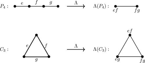
We begin with the definition: Given a graph G with at least one edge, the line graph L(G) is that graph whose vertices are the edges of G, with two of these vertices being adjacent if the corresponding edges are adjacent in G. The operation of going from adjacent edges in G to adjacent vertices in L(G) is indicated in Figure 1.

Figure 1. The operation of forming the line graph.

Some of the early significant results were the following facts about isomorphism of connected nontrivial graphs:

• If G is a connected graph satisfying $G\cong L(G),$ then G is a cycle.

• If G and H are non-isomorphic connected graphs for which $L(G)\cong L(H),$ then one is the complete graph K₃ and the other is the complete bipartite graph $K_{1,3}.$

Perhaps the most basic question about line graphs is which graphs are indeed line graphs, and in the only paper that Krausz published, he gave a powerful characterization. Many of the interesting properties of graphs also apply to line graphs, and some for which there the most interesting results (including generalizations of the two already mentioned) are the following:

• Isomorphisms

• Characterizations

• Eulerian and Hamiltonian properties

• Distance

• Connectivity

• Planarity

• Colorability

• Matrices

Not surprisingly, there is a natural directed counterpart to a line graph, in which the line digraph L(D) has an arc ab if the digraph D has two arcs a = uv and b = vw. It turns out that the theory of these structures is quite different to that of the undirected line graphs, but we do not develop that theory here. Additionally, there is a wide variety of variations and generalizations of line graphs themselves. In this paper, we have chosen to present two disparate topics. The first is a survey of the complexity of algorithms for topics such as determining whether a graph is actually a line graph or not, and if it is, to find a graph for which it is the line graph. The second is related to our generalization of line graph (to which we gave the name super line graph), and is in fact essentially just an elementary number theory problem.

We close this section with the well-known result that gives several equivalent characterizations of line graphs. For a detailed proof, see [10]. A triangle in a graph G is called odd if some vertex of G is adjacent to an odd number of vertices of the triangle, and it is called even otherwise.

Theorem 1.1.

The following statements are equivalent for a graph $G:$

1. G is the line graph of some graph.

2. (Krausz [20]) The edges of G can be partitioned into complete subgraphs in such a way that no vertex belongs to more than two of the subgraphs.

3. (van Rooij and Wilf [26]) The graph $K_{1,3}$ is not an induced subgraph of G, and if uvw and vwx are both odd triangles, then u and x are adjacent.

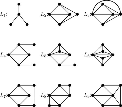
4. (Beineke [9]) None of the nine graphs in Figure 2 is an induced subgraph of G.

   Figure 2. The nine line-forbidden graphs.

   

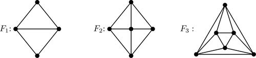
As discussed in the proof of the line graph characterization [10], if G is a line graph containing two even triangles with a common edge, then G must be isomorphic to one the three line graphs F₁, F₂, or F₃ in Figure 3. We shall use this property in Section 2. We observe that F₁ is the line graph of the graph $K_{1,3}$ with an added edge, F₂ is the line graph of F₁, and $F_3=L(K_4).$

Figure 3. Three important line graphs.

2. Complexity of recognizing line graphs and variations of line graphs

The characterization of line graphs (Theorem 1.1) led several authors to investigate efficient algorithms for the recognition of line graphs. In this section we discuss such algorithms, as well as recognition questions for some generalizations and variations of line graphs. We will see that while there are several polynomial algorithms for the recognition of line graphs, similar questions for some generalizations of line graphs remain open. We will also discuss a variation on the line graph theme for which the recognition problem turns out to be NP-complete.

Consider a graph G with m edges and n vertices. The line graph recognition problem seeks to determine if G is a line graph, and if it is, to construct a root graph H so that L(H) = G.

Since the nine forbidden subgraphs in the Beineke characterization have at most six vertices, it follows that a line graph can be recognized in polynomial time with an algorithm that has complexity $O(n^6).$

In 1973, Roussopoulos [25] published a $O($max $\{m,n\})$ algorithm to find a graph H for which L(H) = G. Soon afterwards, Lehot [21] independently discovered an $m+O(n)$ algorithm. Both algorithms are based on the characterizations (2) and (3) of Theorem 1.1. Each algorithm takes an input graph G and finds whether or not it is a line graph, and if it is, constructs a root graph H.

We include here an example from Roussopoulos’s paper. We omit some details and refer the reader to [25] for a complete description.

Roussopoulos’s algorithm takes an input graph G and uses the Krausz condition (2) in Theorem 1.1 to find a partition of the edges of G into complete subgraphs in such a way that no vertex belongs to more than two of the subgraphs.

• Step 1. Begin the algorithm by selecting an edge e and find the number of triangles r (the r-value) that contain e. According to the algorithm, if r = 0, then e = K₂ is a complete graph in the partition. If r = 1, then the other two edges in this triangle are checked for their corresponding r-value. If all of the r-values are 1, then this triangle is a complete graph in the partition. Otherwise, this step is repeated with an edge that has r-value greater than 1. Finally, if $r\ge 2,$ then move to Step 2. In Figure 4, we select e = 13. There are r = 3 triangles 132, 134 and 135 containing e.

  Figure 4. An input graph for Roussopoulos’s algorithm.

  

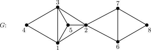
• Step 2. We find the number s of odd triangles that contain e. From our remarks in the last paragraph of Section 1, it follows that if r = 2 and s = 0, then G is one of F₁, F₂ or F₃ or G is not a line graph, which is determined later in the algorithm. If s = r or $s=r-1$ then the s odd triangles form a complete graph $K_{s+2}.$ In all other cases, G is not a line graph. In our example of Figure 4, $s=2=r-1$ with 132 and 135 being the odd triangles, so $K_4=1235$ is a complete graph in the partition.

• Step 3. At this step, we have found one complete graph in the partition. The algorithm proceeds by finding the remaining complete graphs in the partition. For details, see [25]. In our example, the other complete subgraphs are 14, 34, 267, 68 and 78.

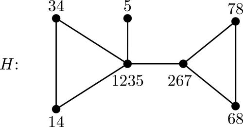
• Step 4. Once the complete graphs are determined, a graph H is constructed by taking one vertex for each complete graph in the partition, and an additional vertex for each vertex in G that belongs to exactly one of the complete graphs in the partition. In our example, we get the graph H with vertices labeled 1235, 14, 34, 267, 68, 78, and 5. The edges in H then join sets that have nonempty intersection. See Figure 5.

  Figure 5. The root graph constructed by Roussopoulos’s algorithm.

  

Roussopoulos [25] shows that for a graph G with m edges and n vertices, the complexity of the algorithm is $O($max $\{m,n\}).$

Naor and Novick [24] presented a parallel algorithm for the construction of the root graph of a line graph. This algorithm was based on a divide-and-conquer scheme. Degiorgi and Simon [15] published a dynamic algorithm for line graph recognition. Their solution uses the result of Whitney [29] that if G is a connected graph of order at least 5, then the automorphism groups of G and L(G) are isomorphic. See Chapters 2 and 3 of the book Line Graphs and Line Digraphs [10] for more details. The algorithm of Degiorgi and Simon can also check if a local modification in the graph (addition or deletion of a vertex or an edge) preserves the line graph property. It is shown that the addition or deletion of a vertex (or an edge) can be performed in a time proportional to its adjacency list.

In 2015, another efficient line graph recognition algorithm, called ILIGRA (Inverse Line Graph Algorithm), was given by Liu, Trajanovski, and Mieghem [23]. If G is a line graph, then ILIGRA constructs a root graph H in O(n) time. Otherwise, ILIGRA can check in O(m) time whether or not G is a line graph. The authors present a detailed example and a comparative study showing that ILIGRA out-performs the algorithms of Roussopoulos, Lehot, and Degiorgi and Simon.

We next discuss recognition algorithms for some generalizations of line graphs. In a paper published in 1991, Simić [27] presented an algorithm to recognize a certain type of generalized line graph and to output its root graph. For the definition and a discussion of the generalized line graphs, see [10, 14, 27]. The time complexity of Simić’s algorithm is O(m).

Broersma and Hoede [11,12] generalized the concept of line graphs to path graphs. For a graph G, the vertices of L(G) can be considered as paths of G length 1, with two being adjacent if they overlap in a path of length 0 (i.e., a vertex). The path graph $\Lambda (G)$ has the paths of G of length 2 as its vertices, with two adjacent if they overlap in an edge. See Figure 6 for simple examples. We observe that the two overlapping paths may form a triangle. This concept was generalized to paths of a fixed length k > 2.

Figure 6. Path graphs.

Li and Lin [22] provided a characterization of path graphs. As mentioned in their paper, it is not known if there is an efficient algorithm for path graph recognition. We state this as an open problem.

Open Problem 1: Does there exist an efficient algorithm for path graph recognition and its root graph construction?

Brualdi and Massey [13] defined the arc incidence graph AI(G) of a graph G to be the square of the line graph of the incidence graph of G. Hartke and Helleloid [18] gave a linear-time algorithm for recognizing arc incidence graphs and reconstructing a graph with no isolated vertices from its arc incidence graph.

The recognition problem for line digraphs has also been solved. In 1982, Syslo [28] published a linear time algorithm to recognize a line digraph and output its root graph. The algorithm is based on a characterization of line digraphs by Harary and Norman [17].

Among several other generalizations of line graphs, the one that we discuss in the next section is the concept of super line graphs (see the next section for a definition). To our knowledge, a characterization of super line graphs has not been explored. This leads us to our second open problem.

Open Problem 2: Does there exist an efficient algorithm for super line graph recognition and its root graph construction? In particular, it would be interesting to explore this for super line graphs of index 2.

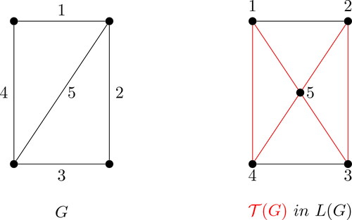
We conclude this section with another variation of line graphs. Triangular line graphs were defined by Jarrett [19]. The triangular line graph $\mathcal{T}(G)$ has the edges of G as vertices, with e and f being adjacent if they lie in a common triangle of G. See Figure 7 for an example. The complexity of triangular line graph recognition was investigated by Anand et al. [1]. It turns out that recognizing a triangular line graph is NP-complete, and the proof is via a reduction from 3-SAT.

Figure 7. Triangular line graph.

3. Super line graphs and line completion numbers

We begin with a simple question about numbers: For example, consider the two numbers r = 27 and s = 45. Assume that $a+b=27$ and $c+d=45$ and define $\alpha (a,c)=\min \{ac,bd\}.$ For example, $\alpha (11,26)=\min \{11·26,16·19\}=\min \{286,304\}=286.$ Question: Given r and s, what is the largest possible value of $\alpha (a,c)$? We denote this by $\beta (r,s):$ $$\beta (r,s)=\max \left\{\min \right\{ac,bd\left\}\right\},$$ where the maximum is taken over all pairs (a, c) with $0\le a\le r,\mathrm{ }0\le c\le s,\mathrm{ }b=r-a,\mathrm{ }d=s-c.$

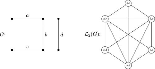
Although others may have considered this question earlier, it came to us through a generalization of line graphs. Given a graph G with at least p edges, the super line graph (of index p) ${\mathcal{L}}_p(G)$ has as its vertices the sets of p edges of G, with two adjacent if there is an edge in one set adjacent to some edge in the other set. An example of a super line graph of index 2 is shown in Figure 8.

Figure 8. An example of a super line graph of index 2.

Given a graph G with p edges, there is of course a natural sequence of super line graphs ${\mathcal{L}}_1(G)(=L(G)),$ ${\mathcal{L}}_2(G),$ …, ${\mathcal{L}}_p(G)=K_1$ ending in the trivial graph. It is not difficult to show that if ${\mathcal{L}}_i(G)$ is complete (with i < p), then so is ${\mathcal{L}}_{i+1}(G).$ Hence there is a least value l for which ${\mathcal{L}}_i(G)$ is complete if and only if $l\le i\le p,$ which we call the line completion number $\text{lc}(G)$ of G.

We begin our discussion of the line completion number with an observation. If a graph G is divided into two disjoint induced subgraphs for which the numbers of edges are m₁ and m₂, then $\text{lc}(G)\ge \min \{m_1,m_2\}$ since clearly G has two disjoint sets of the minimum size having no adjacent edges. We now focus on connected graphs.

Theorem 3.1.

If G is a connected graph with m edges and if l is the greatest number of edges that each of two vertex-disjoint induced subgraphs of G have, then $$l+1\le \text{lc}(G)\le \mathrm{ }\lceil \frac{m}{2}\rceil .$$

The line completion numbers of several families of graphs have been determined, as given in the following theorem [10].

Theorem 3.2.

The line completion numbers of some families of graphs are as follows:

• Complete graphs: $\text{lc}(K_n)=(\begin{array}{c}p\\ 2\end{array})+1$, where $p=\lfloor \frac{n}{2}\rfloor ;$

• Paths and cycles: $\text{lc}(P_n)=\text{lc}(C_n)=\lfloor \frac{n}{2}\rfloor$;

• Fans and wheels: $\text{lc}(F_n)=\text{lc}(W_n)=\lfloor \frac{2n}{3}\rfloor$;

• Windmills: $\text{lc}(M_n)=\lfloor \frac{3n}{4}\rfloor +1.$

• Generalized cubes: $\text{lc}(Q_d)=1+(d-1)2^{d-2}.$

• Grid graphs (with $s\le t$): $$\text{lc}(P_s\times P_t)=\{\begin{array}{cc}s(t-1)-\frac{t}{2}+1\hfill & \text{if}\mathrm{ }s\mathrm{ }\text{is}\mathrm{ }\text{even}\mathrm{ }\text{and}\mathrm{ }t\mathrm{ }\text{is}\mathrm{ }\text{even},\hfill \\ s(t-1)-\frac{t+1}{2}\hfill & \text{if}\mathrm{ }s\mathrm{ }\text{is}\mathrm{ }\text{odd}\mathrm{ }\text{and}\mathrm{ }t\mathrm{ }\text{is}\mathrm{ }\text{odd},\hfill \\ s(t-1)-\frac{t-1}{2}\hfill & \text{if}\mathrm{ }s\text{is}\mathrm{ }\text{even}\mathrm{ }\text{and}\mathrm{ }t\mathrm{ }\text{is}\mathrm{ }\text{odd},\hfill \\ s(t-1)-\frac{t}{2}+1\hfill & \text{if}\mathrm{ }s\text{is}\mathrm{ }\text{odd}\mathrm{ }\text{and}\mathrm{ }t\text{is even}.\hfill \end{array}$$

Readers familiar with the basic families of graphs (even with Kuratowski’s characterization of planar graphs with the two graphs K₅ and $K_{3,3})$ will note that the complete bipartite graphs $K_{r,s}$ are absent from these results. The reason for this is that this is an intriguingly difficult problem in general. Because of the structure of complete bipartite graphs, it turns out that the lower bound of Theorem 1 is important. Since every induced subgraph of a complete bipartite graph is also complete bipartite, this observation can be restated as follows: $$\text{lc}(K_{r,s})=1+\text{max}\{ab:a\le r,b\le s,ab\le (r-a)(s-b)\}.$$

It is therefore useful to introduce this notation: $$\beta (r,s)=\max \left\{\min \right\{ab,(r-a)(s-b)\left\}\right\},$$ where the maximum is taken over all a and b with $0\le a\le r$ and $0\le b\le s.$ This takes us back to the example with which this section was begun. Thus, since $\text{lc}(K_{r,s})=1+\beta (r,s),$ the line completion number of complete bipartite graphs boils down to a purely combinatorial problem, and that is the approach we take here. Hence, in the remainder of the paper, the problem that we concentrate on is simply this:

Find $\beta (r,s)$ for positive integers r and s.

It was not difficult to show that for all p and q, $\beta (2p,2q)=pq$ and a natural conjecture was made in [16] that $\beta (2p,2q+1)=pq$ and that $\beta (2p+1,2q+1)=p(q+1)$ when $p\le q.$ However, when either r or s is odd, and in fact when both are both odd, the conjecture almost never holds.

While the first case is simple (we show that $\beta (r,s)=\frac{1}{4}rs$), the other three cases are more complicated, and therefore more interesting, and in fact we have been unable to find a complete solution in any of those cases. One noteworthy difference between them is what happens in the long run. If r is even and s is odd, then (as we shall show) for fixed r, $\beta (r,s)=\frac{1}{4}r(s-1)$ holds for all but finitely many values of s. However, if both are odd, then there is no comparable formula.

Given r and s, we let $p=\lfloor \frac{r}{2}\rfloor$ and $q=\lfloor \frac{s}{2}\rfloor$ (that is, $r=2p$ or $2p+1$ and $s=2q$ or $2q+1,$ depending on their parity). We define the base case for each of the four types:

• Type I: $r=2p$ and $s=2q,$ with base case (p, q).

• Type II: $r=2p+1$ and $s=2q+1,$ $p\le q,$ with base case $(p,q+1).$

• Type III: $r=2p$ and $s=2q+1,$ with base case (p, q).

• Type IV: $r=2p+1$ and $s=2q,$ with base case again the pair (p, q).

A pair (a, b) is called optimal if $ab=\beta (r,s)$ where $0\le a\le r$ and $0\le b\le s.$ It is easily seen that within each of the four types the product of the two numbers in the base case gives a lower bound for $\beta (r,s).$ One question that we consider is when does equality hold; that is, when is the base case optimal. Here we summarize some of the results.

We now consider the problem in greater detail, assuming that $r\le s$ and exploring the four cases separately, with the bounds being called the base cases. A few results will be proved, but only a few because many of the exact results have lengthy computations. The idea of many proofs is this: If a base case (a, b) (having value ab) does not hold for $\beta (r,s),$ then for some $x\ge 0$ and $y\ge 0,$ it must be that both $(a+x)(b-y)>ab$ and $(a-x)(b+y)>ab.$ Here are the four types of parity (with $r\le s$).

Type I. Both s and t are even. The solution for this type is straightforward: simply split each number in half.

Theorem 3.3.

If $r=2p$ and $s=2q$, then $\beta (r,s)=pq.$

Type II. Let $r=2p+1$ and $s=2q+1$ with $r\le s.$ It turns out that the base case holds some of the time, but not always. A computer program verified that if $r\le 25,$ then the base case holds for all s. However, it does not hold for the pair (27, 45), where the base case is $13·23=299,$ but $\beta (27,45)=300$ ($=12·25=15·20).$ (In terms of graphs, this says that splitting $K_{27,45}$ into $K_{12,25}$ and $K_{15,20}$ is better for our purposes than splitting it into $K_{13,23}$ and $K_{14,22},$ and consequently $\text{lc}(K_{27,45})=301.$)

The main results known are that sometimes the base case holds and sometimes it doesn’t (and there are some pairs for which it is not known). The most important fact here is that for fixed r, eventually the base case never holds.

Theorem 3.4.

Let $r=2p+1$ and $s=2q+1$, with $13\le p\le q.$

1. If $q\le 2p+1$, then the base case holds (that is, $\beta (r,s)=p(q+1)$), for $s=r,r+1,\dots ,r+6$ and $s=2r-3,2r-2,\dots ,2r+1.$

2. If $q\ge 2p+2$, then the base case never holds.

There are in fact some sporadic values other than those given in the theorem for which the solution is known.

Type III. r is even and s is odd with r < s. In this case, for fixed r, the base case eventually holds.

Theorem 3.5.

Let $s=2p$ and $t=2q+1$ with $p\le q$. If p is odd and $q\ge \frac{{(p-1)}^2}{2}$ or if p is even and $q\ge \frac{(p-1)(p-2)}{2}$, then the base case $\beta (r,s)=pq$ holds. Furthermore, the bounds on q are sharp.

There are again some sporadic values other than those given in the theorem for which the result is known.

Type IV. r is odd and s is even with r < s, thus, we assume that $r=2p+1$ and $s=2q$ with q > p. Under these conditions, for fixed s, the base case only holds for the least value of s.

Theorem 3.6.

Let $r=2p+1$ and $s=2q$ with p < q.

1. If $q=p+1$, then the base case $\beta (r,s)=pq$ holds.

2. If $q\ge p+2$, then $\beta (r,s)>pq.$

We observe that not only does the base case not always hold, but there are values of s and t for which it is off by an arbitrarily large amount. In fact, the following result shows that $\beta (r,s)$ can exceed the base case by nearly $\frac{1}{2}{r}^2.$ This follows from the fact that if $r=2p+1$ and $s=2q=2r(r-2),$ then $\beta (r,s)=pq+2p^2-p.$

Determining the exact value of $\beta (r,s)$ in any of the three Types other than when both r and s are even seems to be a formidable, if not impossible, task, even determining all those pairs for which the bisection number is the base case. What we have found however is what eventually happens when the smaller number is fixed. We summarize this in the accompanying table.

Table

r	s	Base case
Even	Even	Always holds
Odd	Odd	Never holds for $s\ge 2r+3$
Even	Odd	Always holds beyond some critical value $s\ge s_0(r)$
Odd	Even	Holds only for $s=r+1$

It follows that if the smaller of the numbers r and s is even, then the base value is known to hold in all but a finite number of cases, while if the smaller number is odd, then the base value is known to hold in only a finite number of cases. The exact value of $\beta (s,t)$ is known for a variety of pairs for which it is not the base value, and we refer the reader to [8] for many of these.

To conclude this section, we return to our original problem, namely, super line graphs and the line completion number. (Recall that $\text{lc}(K_{r,s})=\beta (r,s)+1.$) The following theorem is a summary of key results on this topic, focusing on what eventually happens when the size of the smaller partite set is fixed.

Theorem 3.7.

The line completion number $\text{lc}(K_{r,s})$ of the complete r-by-s bipartite graph with r fixed and $s\ge r$ satisfies the following:

1. For r even,

   1. if s is also even, then $\text{lc}(K_{r,s})=\frac{1}{4}rs+1$ for all $s;$

   2. if s is odd, then $\text{lc}(K_{r,s})=\frac{1}{4}r(s-1)+1$ for $$\{\begin{array}{c}s\ge \frac{1}{4}(r^2-6r+12) if r\equiv 0 (\mathrm{mod} 4),\hfill \\ s\ge \frac{1}{4}(r^2-4r+8) if r\equiv 2 (\mathrm{mod} 4).\hfill \end{array}$$

2. For r odd,

   1. if s is even, then $\text{lc}(K_{r,s})\ge \frac{1}{4}s(r-1)+2$ for all $s\ge r+3;$

   2. if s is also odd, then $\text{lc}(K_{r,s})\ge \frac{1}{4}(r-1)(s+1)+2$ for all $s\ge 2r+3.$

Even though there is much left undone on the problem of the line completion number of complete bipartite graphs, one can find some interesting facts about the corresponding problem for some types of complete tripartite graphs. We note first that, as with complete bipartite graphs, every induced subgraph of a complete tripartite graph is of the same type (allowing for degenerate cases). Therefore, the line completion number of a complete tripartite graph G will be just 1 greater than the number of edges in the lesser of the two induced subgraphs when the vertex set V(G) has been optimally partitioned.

For example, consider the graph $K_{3,4,5}$ with its 12 vertices and 47 edges. Its solution (its “beta value,” 1 less than its line completion number) turns out to be 11, the number of edges in $K_{1,2,3},$ with its counterpart being $K_{2,2,2}$ and its 12 edges.

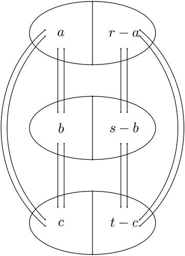
A tripartite graph is naturally composed of three bipartite graphs having its partite sets of vertices belonging to two. For complete tripartite graphs this is indicated in Figure 9, with a corresponding partition of its vertices. Notation-wise, a subgraph of the graph $K_{r,s,t}$ is taken to have a vertices from the set of r, b from the set of s, and c from the set of t, with all of the remaining vertices of course being in the other subgraph.

Figure 9. $K_{r,s,t}.$

We have the following result:

For positive integers r, s, and t, $$\beta (r,s,t)=\max \left\{\min \right\{ab+ac+bc,a\prime b\prime +a\prime c\prime +b\prime c\prime \left\}\right\},$$ where the maximum is taken over all triples (a, b, c) with $0\le a\le r,0\le b\le s,0\le c\le t,a+a\prime =r,b+b\prime =s,c+c\prime =t.$

Start with $K_{r,s,t}$ with $r\le s\le t.$ Then there are eight cases of various combinations of parities:

Table

Type I:	Even	Even	Even
Type II:	Even	Even	Odd
Type III:	Even	Odd	Even
Type IV:	Even	Odd	Odd
Type V:	Odd	Even	Even
Type VI:	Odd	Even	Odd
Type VII:	Odd	Odd	Even
Type VIII:	Odd	Odd	Odd

In numerical format (with values), this would be

Table

2a	2b	2c	$a\le b\le c$
2a	2b	$2c+1$	$a\le b\le c$
2a	$2b+1$	2c	$a\le b<c$
2a	$2b+1$	$2c+1$	$a\le b\le c$
$2a+1$	2b	2c	$a<b\le c$
$2a+1$	2b	$2c+1$	$a<b\le c$
$2a+1$	$2b+1$	2c	$a\le b<c$
$2a+1$	$2b+1$	$2c+1$	$a\le b\le c$

In the case of nearly equal values with the above inequalities (that is, in nondecreasing order), there are these eight cases (probably not all of equal interest).

Table

2k	2k	2k
2k	2k	$2k+1$
2k	$2k+1$	$2k+2$
2k	$2k+1$	$2k+1$
$2k+1$	$2k+2$	$2k+2$
$2k+1$	$2k+2$	$2k+3$
$2k+1$	$2k+1$	$2k+2$
$2k+1$	$2k+1$	$2k+1$

For the eight cases above, we have the following conjectures.

Conjecture 1.

$$\beta (2k,2k,2k)=3k^2.$$

Conjecture 2.

$$\beta (2k,2k,2k+1)=kk+kk+kk=3k^2.$$

Conjecture 3.

$$\beta (2k,2k+1,2k+2)=(k+1)k+(k+1)k+kk=3k^2+2k.$$

Conjecture 4.

$$\beta (2k,2k+1,2k+1)=\beta (2k,2k+1,2k+2)=kk+k(k+1)+k(k+1)=3k^2+2k.$$

Conjecture 5.

$$\beta (2k+1,2k+2,2k+2)=k(k+1)+k(k+1)+(k+1)(k+1)=3k^2+4k+1.$$

Conjecture 6.

$$\beta (2k+1,2k+2,2k+3)=k(k+1)+k(k+2)+(k+1)(k+2)=3k^2+6k+2.$$

Conjecture 7.

$$\begin{array}{c}\beta (2k+1,2k+1,2k+2)=\beta (2k+1,2k+2,2k+2)\\ =k(k+1)+k(k+1)+(k+1)(k+1)=3k^2+4k+1.\end{array}$$

Conjecture 8.

$$\begin{array}{c}\beta (2k+1,2k+1,2k+1)=\beta (2k,2k+1,2k+2)\\ =\beta (2k,2k+1,2k+1)=kk+k(k+1)+k(k+1)=3k^2+2k.\end{array}$$

These are the basic problems that we pose for the reader, with discussion and proofs of some, beginning with the first, which we prove in the general case. Note that this is in the same spirit as the bipartite problem.

Theorem 3.8.

For $a\le b\le c,\beta (2a,2b,2c)=ab+ac+bc.$

Proof.

The proof is by contradiction. We want to show that the partition $[\mathit{abc},\mathit{abc}]$ is optimal. Suppose this is not the case. Then there are integers x, y, and z for which a partition such as $[(a-x)(b-y)(c+z),(a+x)(b+y)(c-z)]$ achieves β. For simplicity, we denote this partition as $[--+,++-].$ Clearly the partition $[---,+++]$ is worse than the base partition. It is easily seen that there are three possible cases to consider. These correspond to partitions $[--+,++-].$ $[-+-,+-+],$ and $[+--,-++].$ We consider the first case. The others are similar, and so we do not include their proofs here.

In the first case, we must have $$(a-x)(b-y)+(a-x)(c+z)+(b-y)(c+z)>ab+ac+bc$$ and $$(a+x)(b+y)+(a+x)(c-z)+(b+y)(c-z)>ab+ac+bc.$$

These can be rewritten as $$(xy-xz-yz)-a(y-z)-b(x-z)-c(x+y)>0$$ and $$(xy-xz-yz)+a(y-z)+b(x-z)+c(x+y)>0.$$

Adding these two yields, $xy>z(x+y)$ and hence x > z and y > z.

It follows that

$(xy-xz-yz)>a(y-z)+b(x-z)+c(x+y)\ge x(y-z)+y(x-z)+z(x+y)$ which simplifies to $0>xy+xz+yz,$ a contradiction. □

Whereas we have the general theorem in which all three sets in a complete tripartite graph are even, the problem in which all three are odd is a difficult problem, analogous to the bipartite problem. Here we do establish the value when all three sets have the same size. This proves one part of Conjecture 8.

Theorem 3.9.

$$\beta (2k+1,2k+1,2k+1)=k(3k+2).$$

The theorem follows from this lemma:

Lemma 1.

Let G be the regular complete tripartite graph $K_{r,r,r}$ with $r=2k+1$, and assume that $\beta (G)=ab+bc+ac$ for the positive integers $a\le b\le c$. Then $c\le a+1.$

Proof

: The proof is by contradiction. We denote r – a, r – b, and r – c by $a\prime ,b\prime ,$ and $c\prime$ respectively. Suppose that a, b, c are such that $\beta (G)=ab+bc+ac,$ with $c-a\ge 2.$ Then, be definition $ab+bc+ac\le a\prime b\prime +b\prime c\prime +a\prime c\prime .$ We consider two cases.

• Case 1: a < b < c. Consider the triple $(a+1,b,c-1).$ Then its corresponding subgraph has $(a+1)b+b(c-1)+(a+1)(c-1)=ab+bc+ac+c-a-1$ edges, which exceeds $\beta (G).$ Also, the second subgraph for this partition has $(a\prime -1)b\prime +b\prime (c\prime +1)+(a\prime -1)(c\prime +1)=a\prime b\prime +b\prime c\prime +a\prime c\prime -c\prime +a\prime -1$ which is at least as large as the number of edges in the first subgraph. This contradicts the hypothesis.

• Case 2: $a<b=c$ or $a=b<c.$ Since these two subcases are so similar, we prove only the first one here. By our assumption, $b\ge a+2.$ Consider the triple $(a+1,b-1,c).$ Its corresponding subgraph has $(a+1)(b-1)+(a+1)c+(b-1)c=ab+bc+ac+b-a-1$ edges which exceeds $\beta (G).$ As in Case 1, the number of edges in the second subgraph of this partition is at least as large as that in the first subgraph. This again contradicts the hypothesis, which completes the proof. □

It now follows from the lemma that a and c differ by at most 1, and from this we see at once that we must have a = b=k and $c=k+1,$ completing the proof of the theorem.

Another interesting result in the bipartite family is the fourth type, (r, s) with r odd and s even. It is rather surprising that for $r=2p+1$ and $s=2q$ the only time that the base case holds is when $q=p+1.$ For example, $\beta (11,12)=5·6=30,$ but $\beta (11,14)\ne 5·7,$ but rather 36 with the pair (6, 6). Extending these ideas to the tripartite case is an open problem, another that we leave to the reader. The accompanying table gives some results for the tripartite case for r = 11, with at least one of s and t even.

Table

r	s	t	β	a	b	c
11	11	12	96	5	6	6
11	12	12	96	5	6	6
11	11	14	107	5	6	7
11	12	13	107	5	6	7
11	12	14	108	6	6	6
11	13	14	119	5	7	7
11	14	14	120	7	6	6

The fact that a complete tripartite graph is composed of three complete bipartite graphs suggests the intriguing question of asking whether there are interesting connections between β parameters; in particular, is $\beta (r,s,t)$ related to the sum $\beta (r,s)+\beta (r,t)+\beta (s,t)$?

The simplest case is of course that in which all of the partite sets are even, for there we have simple equality: $$\beta (2a,2b,2c)=\beta (2a,2b)+\beta (2a,2c)+\beta (2b,2c)(=ab+ac+bc).$$

However, there are examples in which the two quantities and not equal and the inequalities run in different directions. As we have observed, $\beta (11,11)=\beta (11,12)=30$ and $\beta (11,11,12)$ = 96, and therefore $\beta (r,s,t)>\beta (r,s)+\beta (r,t)+\beta (s,t)$ in this case. On the other hand, $\beta (13,13)=42,\beta (13,15)=48$ while $\beta (13,13,15)$ = 133, and therefore $\beta (r,s,t)<\beta (r,s)+\beta (r,t)+\beta (s,t)$ in this case. So this leaves quite a few questions for readers interested in these concepts.

In closing, it would be interesting to extend some of the above results to complete n-partite graphs. We conjecture that Theorems 3.8 and 3.9 hold in the n-partite case.

References

- Anand, P., Escuadro, H., Gera, R., Hartke, S. G., Stolee, D. (2012). On the hardness of recognizing triangular line graphs. Discrete Math. 312(17): 2627–2638.
- Bagga, J. (2004). Old and new generalizations of line graphs. Int. J. Math. Math. Sci. 2004(29): 1509–1521.
- Bagga, J. S., Beineke, L. W. (2021). A survey of line digraphs and generalizations. Discrete Math. Lett. 6: 68–93.
- Bagga, K. S., Beineke, L. W., Varma, B. N. (1995). Super line graphs. In: Alavi, Y., Schwenk, A., eds. Graph Theory, Combinatorics, and Applications, Vol. 1. New York: Wiley, pp. 35–46.
- Bagga, K. S., Beineke, L. W., Varma, B. N. (1995). The line completion number of a graph. In: Alavi, Y., Schwenk, A., eds. Graph Theory, Combinatorics, and Applications, Vol. 2. New York: Wiley, pp. 1197–1201.
- Bagga, J. S., Beineke, L. W., Varma, B. N. (1999). Independence and cycles in super line graphs. Australas. J. Combin. 19: 171–178.
- Bagga, J. S., Beineke, L. W., Varma, B. N. (1999). The super line graph L2. Discrete Math. 206: 51–61.
- Bagga, J. S., Beineke, L. W., Varma, B. N. (2016). A number theoretic problem on super line graphs. AKCE Int. J. Graphs Comb. 13(2): 177–190.
- Beineke, L. W. (1970). Characterizations of derived graphs. J. Combin. Theory. 9(2): 129–135.
- Beineke, L. W., Bagga, J. S. (2021). Line Graphs and Line Digraphs. Switzerland: Springer.
- Broersma, H. J., Hoede, C. (1989). Path graphs. J. Graph Theory. 13(4): 427–444.
- Broersma, H. J., Li, X. (2002). Isomorphisms and traversability of directed path graphs. Discuss. Math. Graph Theory. 22(2): 215–228.
- Brualdi, R. A., Massey, J. J. Q. (1993). Incidence and strong edge colorings of graphs. Discrete Math. 122(1–3): 51–58.
- Cvetković, D., Doob, M., Simić, S. (1981). Generalized line graphs. J. Graph Theory. 5(4): 385–399.
- Degiorgi, D. G., Simon, K. (1995). A dynamic algorithm for line graph recognition In: Nagl, M., ed. Graph-Theoretic Concepts in Computer Science. WG 1995. Lecture Notes in Computer Science, Vol. 1017. Berlin: Springer-Verlag, pp. 37–48.
- Gutiérrez, A., Lladó, A. S. (2002). On the edge-residual number and the line completion number of a graph. Ars Combin. 63: 65–74.
- Harary, F., Norman, R. Z. (1960). Some properties of line digraphs. Rend. Circ. Mat. Palermo. 9(2): 161–168.
- Hartke, S. G., Helleloid, G. T. (2012). Reconstructing a graph from its arc incidence graph. Graphs Combin. 28(5): 637–652.
- Jarrett, E. B. (1995). On iterated triangular line graphs. In: Alavi, Y., Schwenk, A. eds. Graph Theory, Combinatorics, and Applications, Vol. 1. New York: Wiley, pp. 589–599.
- Krausz, J. (1943). Démonstration nouvelle d’un théorème de Whitney sur les réseaux (Hungarian with French summary). Mat. Fiz. Lapok. 50: 75–85.
- Lehot, P. G. H. (1974). An optimal algorithm to detect a line graph and output its root graph. J. ACM. 21(4): 569–575.
- Li, H., Lin, Y. (1993). On the characterization of path graphs. J. Graph Theory. 17(4): 463–466.
- Liu, D., Trajanovski, S., Van Mieghem, P. (2015). ILIGRA: an efficient inverse line graph algorithm. J. Math. Model. Algorithms. 14(1): 13–33.
- Naor, J., Novick, M. B. (1990). An efficient reconstruction of a graph from its line graph in parallel. J. Algorithms. 11(1): 132–143.
- Roussopoulos, N. D. (1973). A max {m, n} algorithm for determining the graph H from its line graph G. Inf. Process. Lett. 2(4): 108–112.
- Rooij, A. C. M., Wilf, H. S. (1965). The interchange graph of a finite graph. Acta Math. Acad. Sci. Hungar. 16(3–4): 263–269.
- Simić, S. (1991). An algorithm to recognize a generalized line graph and output its root graph. Publ. Inst. Math. 49(63): 21–26.
- Syslo, M. M. (1982). A labeling algorithm to recognize a line digraph and output its root graph. Inform. Process. Lett. 15(1): 28–30.
- Whitney, H. (1932). Congruent graphs and the connectivity of graphs. Amer. J. Math. 54(1): 150–168.
- Whitney, H. (1933). 2-Isomorphic graphs. Amer. J. Math. 55(1/4): 245–254.