Exact square coloring of graphs resulting from some graph operations and products

Abstract

A vertex coloring of a graph $G=(V,E)$ is called an exact square coloring of G if any pair of vertices at distance 2 receive distinct colors. The minimum number of colors required by any exact square coloring is called the exact square chromatic number of G and is denoted by ${\chi }^{[\#2]}(G).$ A set of vertices is called an exact square clique of G if any pair of vertices of the set are at distance 2. The exact square clique number of G, denoted by ${\omega }^{[\#2]}(G),$ is the maximum cardinality of an exact square clique of G and clearly, ${\omega }^{[\#2]}(G)\le {\chi }^{[\#2]}(G).$ In this article, we give tight upper bounds of the exact square chromatic number of various standard graph operations, including the Cartesian product, strong product, lexicographic product, corona product, edge corona product, join, subdivision, and Mycielskian of a graph. We also present tight lower bounds of the exact square clique number of these graph operations.

Keywords:

• Exact square coloring
• Cartesian product
• strong product
• corona product
• Mycielskian

1. Introduction

For a positive integer p, a p-distance coloring of a given graph $G=(V,E)$ is an assignment of colors to V(G) such that any pair of vertices at distance at most p receive distinct colors. The concept of p-distance coloring has been studied extensively since its introduction in 1969 by Kramer and Kramer [7, 8]. For a positive integer p, an exact p-distance coloring of G is an assignment of colors to V(G) such that any pair of vertices at distance exactly p receive distinct colors. The exact p-chromatic number of G is the minimum number of colors used by an exact p-coloring of G and is denoted by ${\chi }^{[\#p]}(G).$ Note that an exact p-coloring of G is equivalent to a proper vertex coloring of exact distance p-power of G, which is denoted by $G^{[\#p]},$ and obtained by taking the vertices of G and adding an edge between a pair of vertices only if they are at distance p in G. It is clear that ${\chi }^{[\#p]}(G)=\chi (G^{[\#p]}).$

In this article, we investigate exact p-distance coloring with p = 2. Given a graph $G=(V,E),$ an exact square coloring of G is an assignment of colors to V(G) such that any pair of vertices at distance two receive distinct colors. The exact square chromatic number of G, denoted by ${\chi }^{[\#2]}(G),$ is the minimum number of colors required by an exact square coloring of G. Foucaud et al. [6] examined the exact square coloring of subcubic planar graphs. They obtained tight upper bound on ${\chi }^{[\#2]}(G)$ for subcubic bipartite planar graphs and showed that for triangle-free graphs, exact square coloring is same as injective coloring. An injective coloring of a graph is a vertex coloring such that any pair of vertices having a common neighbor receives distinct colors. Panda and Priyamvada [12] proved complexity results for some subclasses of bipartite graphs, which can be re-interpreted as results on exact square coloring.

Interestingly, exact square coloring of a graph is equivalent to its L(0, 1)-labelling, which is a particular case of the well-studied L(p, q)-labelling of a graph. A L(p, q)-labelling of a graph G for non-negative integers p and q is defined as a labelling f of V(G) such that $|f(x)-f(y)|\ge p,$ if x and y are adjacent vertices and $|f(x)-f(y)|\ge q,$ if x and y are at distance 2. L(p, q)-labelling of various families of graphs has been widely studied by many researchers, including digraphs [4], planar graphs [5], square of paths [20], subdivision of graphs [3], and products of complete graphs [9]. In particular, L(2, 1)-labelling has been extensively investigated over the last decades, for instance see [2, 11, 14, 17, 19]. Moreover, Liu et al. [10] examined the L(1, 2)-labelling numbers on square of cycles, and L(0, 1)-labelling on interval graphs with its application on the radio frequency assignment problem was studied in [15].

Exact square coloring also appears in literature with another name as strong subcoloring. Shalu et al. [18] showed that the strong subcoloring problem is NP-complete on bipartite graphs and $K_{1,r}$-free split graphs for r > 3. They also studied the complexity of determining a lower bound of ${\chi }^{[\#2]}(G)$ on bipartite graphs and $K_{1,4}$-free split graphs. We call this lower bound exact square clique number and denote it by $.$ Exact square clique number of a graph G is formally defined as the maximum cardinality of a set of vertices such that each pair of vertices in the set are at distance 2 in G.

Various operations defined over graphs form an important method to both construct new graphs and structurally characterize particular graph classes, for instance union and join in the case of cographs. Many of these operations also play a key role in designing and analysing networks, for example grid graphs as the Cartesian product of paths. Graph products have been widely studied from different perspectives for many graph parameters, for instance, see [13, 19].

In this article, we study some standard graph operations including the Cartesian product, strong product, lexicographic product, corona product, edge corona product, join and Mycielskian of graphs. We give tight bounds of the exact square chromatic number and exact square clique number of graphs under these operations. The formal definitions of these operations are given in the subsequent sections. The part of this article was presented in International conference on graphs, combintorics and optimization [16].

The organization of the article is as follows. In Section 2, we give some pertinent definitions and notations. In Section 3, we give upper bounds of the exact square chromatic number of various graph operations and show that each of these bounds are tight. In Section 4, we give tight lower bounds of the exact square clique number of various graph operations. Some concluding remarks form Section 5.

2. Preliminaries

In this article, we consider simple and connected graphs. Given a graph $G=(V,E),$ for any vertex $v\in V(G),$ N(v) denotes the set of neighbors of v, {$u\in V(G):uv\in E(G)$}. The degree of a vertex v is defined as $d(v)=|N(v)|.$ Let $N_G^2(v)$ denote the set of vertices at distance 2 from v in G. Let n denote the number of vertices of a graph G. For $U\subseteq V,$ the subgraph induced by G on U is denoted by $G[U].$ For any $C\subseteq V,$ if every pair of distinct vertices in C are adjacent in $G[C],$ then C is known as a clique. A set $I\subseteq V$ is called an independent set if no two vertices in I are adjacent in $G[I].$ The clique number of G, denoted by $\omega (G),$ is the maximum cardinality of any clique of G. The clique cover number of G, denoted by $\theta (G),$ is the minimum number of cliques that partition V(G). The independence number of G, denoted by $\alpha (G),$ is the maximum cardinality of an independent set of G. A proper edge coloring of G is an assignment of colors to E(G) such that any pair of adjacent edges receive distinct colors. The chromatic index of G is the minimum number of colors required by a proper edge coloring of G. Let $[k]$ denote the set of integers $\{1,2,\dots ,k\}.$

3. Exact square coloring of graph operations and products

In this section, we study the exact square coloring of graphs under various graph operations and products, and give tight upper bound for each operation.

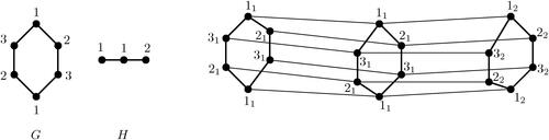
3.1. Cartesian product of graphs

The Cartesian product of two graphs G and H is the graph $G\square H$ with vertices $V(G\square H)=V(G)\times V(H),$ and for which $(g_1,h_1)(g_2,h_2)$ is an edge if g₁ = g₂ and $h_1{h}_2\in E(H),$ or $g_1{g}_2\in E(G)$ and h₁ = h₂. In this subsection, we give tight upper bound on the exact square chromatic number of Cartesian product of two graphs using the L(1,1)-labelling number. Denoted by ${\lambda }_{1,1}(G),$ the L(1,1)-labelling number of a graph $G=(V,E)$ is the minimum number of labels used by a vertex labeling of V(G) such that any pair of vertices at distance at most two receive distinct labels.

Theorem 3.1.

Let G and H be graphs with exact square chromatic number ${\chi }^{[\#2]}(G)$ and ${\chi }^{[\#2]}(H)$, respectively, and L(1,1)-labelling number ${\lambda }_{1,1}(G)$ and ${\lambda }_{1,1}(H)$, respectively. Then, ${\chi }^{[\#2]}(G\square H)\le$ min $\{{\lambda }_{1,1}(G){\chi }^{[\#2]}(H),{\lambda }_{1,1}(H){\chi }^{[\#2]}(G)\}.$

Moreover, the bound is tight. If G and H are complete graphs, then ${\chi }^{[\#2]}(K_{n_1}\square K_{n_2})=$ min $\{n_1,n_2\}.$

Proof.

Without loss of generality, we assume that ${\lambda }_{1,1}(G){\chi }^{[\#2]}(H)\le {\lambda }_{1,1}(H){\chi }^{[\#2]}(G).$ Let c be the optimal L(1,1)-labelling of G and ${\varphi }_H$ be the optimal exact square coloring of H. We define coloring ${\varphi }_{G\square H}$ on $V(G\square H)$ using${\lambda }_{1,1}(G){\chi }^{[\#2]}(H)$ colors as follows.

For every $(g_i,h_j)\in V(G\square H),$ assign ${\varphi }_{G\square H}(g_i,h_j)=c{(g_i)}_{{\varphi }_H(h_j)}.$

We claim that ${\varphi }_{G\square H}$ is an exact square coloring of $G\square H.$ Firstly, recall that $d_{G\square H}((g_1,h_1),(g_2,h_2))=d_G(g_1,g_2)+d_H(h_1,h_2)$ [1]. Thus, we observe that for any pair of vertices (g₁, h₁) and (g₂, h₂), $d_{G\square H}((g_1,h_1),$ $(g_2,h_2))=2,$ if and only if, one of the following holds.

Case 1: $d_G(g_1,g_2)=1=d_H(h_1,h_2)$

In this case, both $g_1{g}_2\in E(G)$ and $h_1{h}_2\in E(H)$ and since c is the L(1,1)-labelling of G, $c(g_1)\ne c(g_2).$ Thus, ${\varphi }_{G\square H}(g_1,h_1)\ne {\varphi }_{G\square H}(g_2,h_2).$

Case 2: $d_G(g_1,g_2)=2$ and h₁ = h₂

In this case, since c is the L(1,1)-labelling of G and $d_G(g_1,g_2)=2,$ we get that $c(g_1)\ne c(g_2)$ and thus, ${\varphi }_{G\square H}(g_1,h_1)\ne {\varphi }_{G\square H}(g_2,h_1).$

Case 3: $d_H(h_1,h_2)=2$ and g₁ = g₂

In this case, we see that ${\varphi }_H(h_1)\ne {\varphi }_H(h_2)$ since ${\varphi }_H$ is an exact square coloring of H and $d_H(h_1,h_2)=2.$ Hence, ${\varphi }_{G\square H}(g_1,h_1)\ne {\varphi }_{G\square H}(g_1,h_2).$

From above, it can be concluded that ${\varphi }_{G\square H}$ is an exact square coloring of $G\square H$ and hence, ${\chi }^{[\#2]}(G\square H)\le {\lambda }_{1,1}(G){\chi }^{[\#2]}(H).$

Similarly, in the case when ${\lambda }_{1,1}(G){\chi }^{[\#2]}(H)\ge {\lambda }_{1,1}(H){\chi }^{[\#2]}(G),$ we can define ${\varphi }_{G\square H}$ on $V(G\square H)$ using ${\lambda }_{1,1}(H){\chi }^{[\#2]}(G)$ colors by assigning ${\varphi }_{G\square H}(g_i,h_j)=c{(h_j)}_{{\varphi }_G(g_i)},$ where ${\varphi }_G$ is the optimal exact square coloring of G and c be the optimal L(1,1)-labelling of H. It can be easily shown that ${\varphi }_{G\square H}$ is an exact square coloring of $G\square H$ and ${\chi }^{[\#2]}(G\square H)\le {\lambda }_{1,1}(H){\chi }^{[\#2]}(G).$

Therefore, ${\chi }^{[\#2]}(G\square H)\le$ min $\{{\lambda }_{1,1}(G){\chi }^{[\#2]}(H),{\lambda }_{1,1}(H){\chi }^{[\#2]}(G)\}.$

Finally, suppose that $G=K_{n_1}$ and $H=K_{n_2}$ with $n_1\le n_2.$ Let $V(G)=\{g_1,\dots ,g_{n_1}\}$ and $V(H)=\{h_1,\dots ,h_{n_2}\}.$ Consider the set $S\subseteq V(G\square H),$ where $S=\{(g_1,h_1),(g_2,h_2),\dots ,(g_{n_1},h_{n_1})\}.$ Observe that every pair of vertices in S are at distance 2 in $G\square H.$ Thus, ${\chi }^{[\#2]}(G\square H)\ge n_1.$ Further, from above, we get that ${\chi }^{[\#2]}(G\square H)\le$ min $\{{\lambda }_{1,1}(K_{n_1}){\chi }^{[\#2]}(K_{n_2}),{\lambda }_{1,1}(K_{n_2}){\chi }^{[\#2]}(K_{n_1})\}$ = min $\{n_1,n_2\}$ = n₁. Therefore, we deduce that ${\chi }^{[\#2]}(K_{n_1}\square K_{n_2})=n_1.$ □

The exact square coloring of $C_6\square P_3$ using 6 colors is illustrated in Figure 1. The following corollary shows that the upper bound is tight.

Figure 1. The exact square coloring of $C_6\square P_3.$

Open Question: Characterize the graphs for which the bound in Theorem 3.1 is tight.

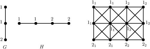
3.2. Strong product of graphs

In this subsection, we give tight upper bound on the exact square chromatic number of strong product of two graphs. The strong product of two graphs G and H is the graph $G⊠H$ with vertices $V(G⊠H)=V(G)\times V(H),$ and for which $(g_1,h_1)(g_2,h_2)$ is an edge if g₁ = g₂ and $h_1{h}_2\in E(H),$ or $g_1{g}_2\in E(G)$ and h₁ = h₂, or $g_1{g}_2\in E(G)$ and $h_1{h}_2\in E(H).$

Theorem 3.2.

Let G and H be graphs with exact square chromatic number ${\chi }^{[\#2]}(G)$ and ${\chi }^{[\#2]}(H)$, respectively. Then, ${\chi }^{[\#2]}(G⊠H)\le {\chi }^{[\#2]}(G){\chi }^{[\#2]}(H).$

Moreover, the bound is tight. If G and H are paths, then ${\chi }^{[\#2]}(P_2⊠P_{n_1})=2$ and ${\chi }^{[\#2]}(P_{n_1}⊠P_{n_2})=4$ for $n_1,n_2\ge 3.$

Proof.

Let ${\varphi }_G$ be the optimal exact square coloring of G and ${\varphi }_H$ be the optimal exact square coloring of H. We define coloring ${\varphi }_{G⊠H}$ on $V(G⊠H)$ using ${\chi }^{[\#2]}(G){\chi }^{[\#2]}(H)$ colors as follows.

For every $(g_i,h_j)\in V(G⊠H),$ assign ${\varphi }_{G⊠H}(g_i,h_j)={\varphi }_G{(g_i)}_{{\varphi }_H(h_j)}.$

We claim that ${\varphi }_{G⊠H}$ is an exact square coloring of $G⊠H.$ Note that $d_{G⊠H}((g_1,h_1),(g_2,h_2))=$ max $\{d_G(g_1,g_2),d_H(h_1,h_2)\}$ [1] for any pair of vertices (g₁, h₁) and (g₂, h₂). Thus, $d_{G⊠H}((g_1,h_1),(g_2,h_2))=2,$ if and only if, either $d_G(g_1,g_2)=2,$ or $d_H(h_1,h_2)=2,$ or both $d_G(g_1,g_2)=2=d_H(h_1,h_2).$ In each of these cases, since ${\varphi }_G$ and ${\varphi }_H$ are exact square colorings, either ${\varphi }_G(g_1)\ne {\varphi }_G(g_2),$ or ${\varphi }_H(h_1)\ne {\varphi }_H(h_2),$ or both ${\varphi }_G(g_1)\ne {\varphi }_G(g_2)$ and ${\varphi }_H(h_1)\ne {\varphi }_H(h_2).$ This implies that for any pair of vertices that are distance 2 apart in $G⊠H,{\varphi }_{G⊠H}(g_1,h_1)\ne {\varphi }_{G⊠H}(g_2,h_2).$ Thus, ${\varphi }_{G⊠H}$ is an exact square coloring of $G⊠H$ using ${\chi }^{[\#2]}(G){\chi }^{[\#2]}(H)$ colors.

Therefore, ${\chi }^{[\#2]}(G⊠H)\le {\chi }^{[\#2]}(G){\chi }^{[\#2]}(H).$

Finally, suppose that G = P₂ and $H=P_{n_1}$ with $n_1\ge 3.$ Let $V(G)=\{g_1,g_2\}$ and $V(H)=\{h_1,\dots ,h_{n_1}\}.$ Observe that $d_{G⊠H}((g_1,h_1),(g_1,h_3))=2.$ Thus, ${\chi }^{[\#2]}(G⊠H)\ge 2.$ Also, the above theorem implies that ${\chi }^{[\#2]}(G⊠H)\le {\chi }^{[\#2]}(P_2){\chi }^{[\#2]}(P_{n_1})=2.$ Hence, we get that ${\chi }^{[\#2]}(G⊠H)=2.$

Now suppose that $G=P_{n_1}$ and $H=P_{n_2}$ with $n_1,n_2\ge 3.$ Let $V(G)=\{g_1,\dots ,g_{n_1}\}$ and $V(H)=\{h_1,\dots ,h_{n_2}\}.$ Consider the set $S\subseteq V(G⊠H),$ where $S=\{(g_1,h_1),(g_3,h_1),(g_1,h_3),(g_3,h_3)\}.$ Observe that every pair of vertices in S are at distance 2 in $G⊠H.$ Thus, ${\chi }^{[\#2]}(G⊠H)\ge 4.$ Further since ${\chi }^{[\#2]}(G⊠H)\le {\chi }^{[\#2]}(G){\chi }^{[\#2]}(H),$ we get that ${\chi }^{[\#2]}(G⊠H)\le {\chi }^{[\#2]}(P_{n_1}){\chi }^{[\#2]}(P_{n_2})=4.$ Therefore, we deduce that ${\chi }^{[\#2]}(G⊠H)=4.$ □

Figure 2 illustrates the exact square coloring of $P_3⊠P_4$ using 4 colors.

Figure 2. The exact square coloring of $P_3⊠P_4.$

Open Question: Characterize the graphs for which the bound in Theorem 3.2 is tight.

3.3. Lexicographic product of graphs

In this subsection, we give tight upper bound on the exact square chromatic number of lexicographic product of two graphs. The lexicographic product of two graphs G and H is the graph $G°H$ with vertices $V(G°H)=V(G)\times V(H),$ and for which $(g_1,h_1)(g_2,h_2)$ is an edge if g₁ = g₂ and $h_1{h}_2\in E(H),$ or $g_1{g}_2\in E(G).$ In other words, $G°H$ is obtained by replacing each vertex g_i of G with H_i, a copy of H such that every vertex of H_i is adjacent to every vertex of H_j whenever g_i and g_j are adjacent in G.

Theorem 3.3.

Let G and H be graphs with exact square chromatic number ${\chi }^{[\#2]}(G)$ and clique cover number $\theta (H)$, respectively. Then, ${\chi }^{[\#2]}(G°H)\le {\chi }^{[\#2]}(G)\theta (H).$

Moreover, the bound is tight. If H = K_n and G is any graph, then ${\chi }^{[\#2]}(G°K_n)={\chi }^{[\#2]}(G).$

Proof.

Let ${\varphi }_G$ be the optimal exact square coloring of G. Let $C_1,C_2,\dots ,C_{\theta (H)}$ represent the cliques that partition V(H). We define coloring ${\varphi }_{G°H}$ on $V(G°H)$ using ${\chi }^{[\#2]}(G)\theta (H)$ colors as follows.

For every $(g_i,h_j)\in V(G°H),$ assign ${\varphi }_{G°H}(g_i,h_j)={\varphi }_G{(g_i)}_k,$ where $h_j\in C_k$ for some $k\in [\theta (H)].$ We claim that ${\varphi }_{G°H}$ is an exact square coloring of $G°H.$ Note that $d_{G°H}((g_1,h_1),(g_2,h_2))=d_G(g_1,g_2),$ if $g_1\ne g_2$ and $d_{G°H}((g_1,h_1),(g_1,h_2))=$ min $\{d_H(h_1,h_2),2\}$ [1], for any pair of vertices (g₁, h₁) and (g₂, h₂). Thus, $d_{G°H}((g_1,h_1),(g_2,h_2))=2,$ if and only if, either $d_G(g_1,g_2)=2,$ or (g₁, h₁) and (g₂, h₂) belong to same copy of H and h₁ and h₂ are in different cliques of H. We conclude that if $d_{G⊠H}((g_1,h_1),(g_2,h_2))=2,$ then ${\varphi }_{G°H}(g_1,h_1)\ne {\varphi }_{G°H}(g_1,h_2),$ since in the first case, ${\varphi }_G$ is an exact square coloring and ${\varphi }_G(g_1)\ne {\varphi }_G(g_2)$ if $d_G(g_1,g_2)=2,$ and in the latter case, h₁ and h₂ belong to different cliques C_k and C_r, $k\ne r.$ Thus, ${\varphi }_{G°H}$ is an exact square coloring of $G°H$ using ${\chi }^{[\#2]}(G)\theta (H)$ colors. Therefore, ${\chi }^{[\#2]}(G°H)\le {\chi }^{[\#2]}(G)\theta (H).$

Finally, suppose that H = K_n with $V(K_n)=\{h_1,\dots ,h_n\}$ and G is any graph with exact square chromatic number ${\chi }^{[\#2]}(G).$ Note that for any pair of vertices $g_i,g_j\in V(G)$ that are at distance 2 in G, $d_{G°H}((g_i,h_1),(g_j,h_1))=2.$ Thus, ${\chi }^{[\#2]}(G°K_n)\ge {\chi }^{[\#2]}(G).$ Further since ${\chi }^{[\#2]}(G°H)\le {\chi }^{[\#2]}(G)\theta (H),$ we get that ${\chi }^{[\#2]}(G°K_n)={\chi }^{[\#2]}(G),$ since $\theta (K_n)=1.$ □

Open Question: Characterize the graphs for which the bound in Theorem 3.3 is tight.

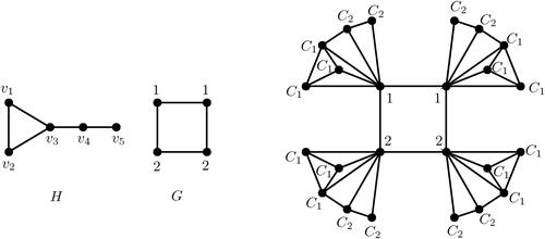
3.4. Corona product of graphs

The corona product of G and H is the graph obtained by taking one copy of G, called the center graph and $|V(G)|$ copies of H, called the outer graph, and making the ith vertex of G adjacent to every vertex of the ith copy of H, where $1\le i\le |V(G)|.$ The corona product of two graphs G and H is denoted by $G·H.$ Now, we give a tight upper bound on the exact square chromatic number of corona product of two graphs.

Theorem 3.4.

Let H be a graph with clique cover number $\theta (H)$ and let G be a graph with exact square chromatic number ${\chi }^{[\#2]}(G)$. Then, ${\chi }^{[\#2]}(G·H)\le \theta (H)+{\chi }^{[\#2]}(G).$

Moreover, the bound is tight. If G is a complete graph, then ${\chi }^{[\#2]}(K_n·H)=\theta (H)+1,$ where $n\ge 2.$

Proof.

Note that an optimal clique cover partitions the set of vertices of graph into cliques. Let $C_1,C_2,\dots ,C_{\theta (H)}$ represent the cliques of H. Let ${\varphi }_G$ be the optimal exact square coloring of G. We define a coloring ${\varphi }_{G·H}$ on $V(G·H)$ using $\theta (H)+{\chi }^{[\#2]}(G)$ colors as follows. $${\varphi }_{G·H}(v)=\{\begin{array}{c}{\varphi }_G(v),\mathrm{ }\text{if}\mathrm{ }v\in V(G)\hfill \\ c_j,\mathrm{ }\text{if}\mathrm{ }v\in V(H)\mathrm{ }\text{and}\mathrm{ }v\in C_j\mathrm{ }\text{for}\mathrm{ }\text{some}j.\hfill \end{array}$$

We claim that ${\varphi }_{G·H}$ is an exact square coloring of $G·H.$ Note that vertices of G and all copies of H receive colors from different color set. For any copy of H, the vertices in different cliques receive distinct colors since they are distance 2 apart in $G·H.$ The vertices of distinct copies of H are at least at distance 3, thus create no conflict. Finally, since ${\varphi }_G$ is an exact square coloring of G, the vertices of G that are at distance 2 receive different colors. Therefore, ${\varphi }_{G·H}$ is an exact square coloring of $G·H$ and thus, ${\chi }^{[\#2]}(G·H)\le \theta (H)+{\chi }^{[\#2]}(G).$

Now, suppose that G = K_n where $n\ge 2.$ It is clear that any exact square coloring of $K_n·H$ requires at least $\theta (H)$ colors. Let us assume that ${\chi }^{[\#2]}(K_n·H)=\theta (H).$ Then there exist an exact square coloring of $K_n·H$ using $\theta (H)$ colors. In the copy of H attached to any $v\in V(K_n),$ it is clear that the vertices in different cliques receive distinct colors. Thus, $\theta (H)$ colors are used by vertices of H attached to $v\in V(K_n)$ in any exact square coloring of $K_n·H.$ But any vertex $v\prime \in V(K_n)\setminus \left\{v\right\}$ cannot receive any color appearing on the vertices of H attached to v, which is a contradiction. Thus, ${\chi }^{[\#2]}(K_n·H)\ge \theta (H)+1.$ Further, since ${\chi }^{[\#2]}(G·H)\le \theta (H)+{\chi }^{[\#2]}(G),$ we get that ${\chi }^{[\#2]}(K_n·H)\le \theta (H)+{\chi }^{[\#2]}(K_n)=\theta (H)+1.$ Therefore, from the above inequalities, we get that ${\chi }^{[\#2]}(K_n·H)=\theta (H)+1.$ □

Figure 3 illustrates the exact square coloring of corona product of C₄ and H, where H is the graph obtained by identifying a pendant vertex of P₃ with any vertex of K₃.

Figure 3. The exact square coloring of corona product of C₄ and H.

Open Question: Characterize the graphs for which the bound in Theorem 3.4 is tight.

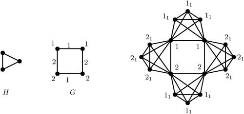
3.5. Edge corona product of graphs

The edge corona product of G and H is the graph obtained by taking one copy of G, called the center graph and $|E(G)|$ copies of H, called the outer graph, and for every edge $e_i=uv\in E(G),$ making u and v of G adjacent to every vertex of the ith copy of H. The edge corona product of two graphs G and H is denoted by $G{·}^{e}H.$ The vertex set of $G{·}^{e}H$ is given by $V(G{·}^{e}H)=V(G)\cup \{v_i^e:1\le i\le |V(H)|$ and $e\in E(G)\}.$ Now, we give a tight upper bound on the exact square chromatic number of edge corona product of two graphs.

Theorem 3.5.

Let G be a graph with exact square chromatic number ${\chi }^{[\#2]}(G)$ and chromatic index $\chi \prime (G)$. Let H be a graph with clique cover number $\theta (H)$. Then, ${\chi }^{[\#2]}(G{·}^{e}H)\le {\chi }^{[\#2]}(G)+\chi \prime (G)\theta (H).$

Moreover, the bound is tight. If H is a complete graph and $G=K_4$, then ${\chi }^{[\#2]}(K_4{·}^e{K}_n)=4$, where $n\ge 2.$

Proof.

Let ${\varphi }_G$ be the optimal exact square coloring of G and $c\prime :E(G)\to [\chi \prime (G)]$ be the proper edge coloring of G. Let $C_1,C_2,\dots ,C_{\theta (H)}$ represent the cliques of H. Now, we define a coloring ${\varphi }_{G{·}^{e}H}$ on $V(G{·}^{e}H)$ using ${\chi }^{[\#2]}(G)+\chi \prime (G)\theta (H)$ colors as follows. $${\varphi }_{G{·}^{e}H}(v)=\{\begin{array}{c}{\varphi }_G(v),\mathrm{ }\text{if}\mathrm{ }v\in V(G)\hfill \\ j_{c\prime (e)},\mathrm{ }\text{if}\mathrm{ }v=v_i^e\in C_j\mathrm{ }\text{for}\mathrm{ }\text{some}\mathrm{ }j.\hfill \end{array}$$

We claim that ${\varphi }_{G{·}^{e}H}$ is an exact square coloring of $G{·}^{e}H.$ It is clear that vertices of G and each copy of H corresponding to edge $e\in E(G)$ receive colors from different color set. Thus, we do not consider any pair of vertices x, y such that $x\in V(G)$ and y belongs to a copy of H. Note that any pair of vertices, $v_i^e$ and $v_j^{e\prime },$ in different copies of H are distance 2 apart if edges e and $e\prime$ are adjacent in G. Since $c\prime$ is a proper edge coloring of G, we get that $c\prime (e)\ne c\prime (e\prime )$ which implies that ${\varphi }_{G{·}^{e}H}(v_i^e)\ne {\varphi }_{G{·}^{e}H}(v_j^{e\prime }).$ Finally, since ${\varphi }_G$ is an exact square coloring of G, the vertices of G that are at distance 2 receive distinct colors. Therefore, ${\varphi }_{G{·}^{e}H}$ is an exact square coloring of $G{·}^{e}H$ and thus, ${\chi }^{[\#2]}(G{·}^{e}H)\le {\chi }^{[\#2]}(G)+\chi \prime (G)\theta (H).$

Finally, suppose that $G=K_4$ and H = K_n with $n\ge 2.$ From above, we get that ${\chi }^{[\#2]}(K_4{·}^e{K}_n)\le {\chi }^{[\#2]}(K_4)+\chi \prime (K_4)\theta (K_n)=4$ since ${\chi }^{[\#2]}(K_4)=1,\chi \prime (K_4)=3$ and $\theta (K_n)=1.$ Thus, ${\chi }^{[\#2]}(K_4{·}^e{K}_n)\le 4.$

Let $V(K_4)=\{v_1,v_2,v_3,v_4\}$ and $E(K_4)=\{v_1{v}_2,v_1{v}_3,v_1{v}_4,v_2{v}_3,v_2{v}_4,v_3{v}_4\}.$ Let $H_{i,j}$ denote the copy of graph H corresponding to edge $v_i{v}_j,i<j.$ Let $u_{i,j}$ be any vertex of the graph $H_{i,j}.$ We claim that ${\chi }^{[\#2]}(K_4{·}^e{K}_n)\ge 4.$ Consider the set $S=\{v_3,u_{1,4},u_{1,2},u_{2,4}\}.$ Note that each pair of vertices in S are at distance 2 from each other. It is clear that ${\chi }^{[\#2]}(K_4{·}^e{K}_n)\ge 4,$ since each vertex of S should receive a distinct color in any exact square coloring of $K_4{·}^e{K}_n.$ Since the exact square coloring ${\varphi }_{K_4{·}^e{K}_n}$ obtained using above arguments uses 4 colors, we conclude that ${\varphi }_{K_4{·}^e{K}_n}$ is an optimal exact square coloring of $K_4{·}^e{K}_n$ and ${\chi }^{[\#2]}(K_4{·}^e{K}_n)=4.$ □

The exact square coloring of $C_4{·}^e{K}_3$ using 4 colors is illustrated in Figure 4.

Figure 4. The exact square coloring of $C_4{·}^e{K}_3.$

Open Question: Characterize the graphs for which the bound in Theorem 3.5 is tight.

3.6. Join and subdivision of a graph

Given two graphs, $G,H\ne K_n,$ the join of G and H, denoted by G + H, is the graph obtained by joining each vertex of G with each vertex of H. Formally, the vertex set of G + H is given by $V(G+H)=V(G)\cup V(H)$ and the edge set of G + H is given by $E(G+H)=E(G)\cup E(H)\cup \{xy:x\in V(G),y\in V(H)\}.$

Theorem 3.6.

Let G + H denote the join of any two graphs G and H with clique cover number $\theta (G)$ and $\theta (H)$, respectively. Then, ${\chi }^{[\#2]}(G+H)$= max $\{\theta (G),\theta (H)\}.$

Proof.

Let G and H be graphs with clique cover number $\theta (G)$ and $\theta (H),$ respectively. Let $k=$ max $\{\theta (G),\theta (H)\}.$ Let $C_1,C_2,\dots ,C_{\theta (G)}$ and $D_1,D_2,\dots ,D_{\theta (H)}$ represent the cliques that partition V(G) and V(H), respectively. Then, we define a coloring ${\varphi }_{G+H}:V(G+H)\to [k]$ as follows. $${\varphi }_{G+H}(v)=\{\begin{array}{c}j,\mathrm{ }\text{if}\mathrm{ }v\in V(G)\mathrm{ }\text{and}\mathrm{ }v\in C_j\mathrm{ }\text{for}\mathrm{ }\text{some}\mathrm{ }j,\hfill \\ i,\mathrm{ }\text{if}\mathrm{ }v\in V(H)\mathrm{ }\text{and}\mathrm{ }v\in D_i\mathrm{ }\text{for}\mathrm{ }\text{some}\mathrm{ }i.\hfill \end{array}$$

We claim that ${\varphi }_{G+H}$ is an exact square coloring of G + H. Note that for any pair of vertices $x,y\in V(G+H),d_{G+H}(x,y)=2,$ if and only if, either x, y both belong to different cliques of G, or x, y both belong to different cliques of H. Thus, ${\varphi }_{G+H}(x)\ne {\varphi }_{G+H}(y)$ and ${\varphi }_{G+H}$ is an exact square coloring of G + H. Clearly, any exact square coloring of G + H requires k colors since any pair of vertices of distinct cliques in G (and H) are distance 2 apart.

Therefore, ${\varphi }_{G+H}$ is an optimal exact square coloring of G + H and ${\chi }^{[\#2]}(G+H)=k.$ □

Let G be any graph. Then, the subdivision graph of G denoted by S(G) is formally defined as $S(G)=(V(S(G)),E(S(G))),$ where $V(S(G))=V(G)\cup E(G)$ and $E(S(G))=\{ve,eu:e=uv\in E(G)\}.$

Theorem 3.7.

Let G be any graph with chromatic number $\chi (G)$ and chromatic index $\chi \prime (G)$. Then, the exact chromatic number of the subdivision graph S(G) is given by ${\chi }^{[\#2]}(S(G))$= max $\{\chi (G),\chi \prime (G)\}.$

Proof.

Let $c:V(G)\to [\chi (G)]$ and $c\prime :E(G)\to [\chi \prime (G)]$ be proper vertex coloring and proper edge coloring of G, respectively. Let $k=$ max $\{\chi (G),\chi \prime (G)\}.$ Now, we define a coloring ${\varphi }_{S(G)}:V(S(G))\to [k]$ as follows. $${\varphi }_{S(G)}(v)=\{\begin{array}{c}i,\mathrm{ }\text{if}\mathrm{ }v\in V(G)\mathrm{ }\text{and}\mathrm{ }c(v)=i,\hfill \\ j,\mathrm{ }\text{if}\mathrm{ }v\in E(G)\mathrm{ }\text{and}\mathrm{ }c\prime (v)=j.\hfill \end{array}$$

Note that $d_{S(G)}(x,y)=2,$ if and only if, either $x,y\in V(G)$ and $xy\in E(G),$ or either $x=e,y=e\prime \in E(G)$ and e is adjacent to $e\prime$ in G. In both the cases, since c and $c\prime$ are proper vertex coloring and proper edge coloring of G, respectively, it is clear that ${\varphi }_{S(G)}$ is an optimal exact square coloring of S(G). Thus, we conclude that ${\chi }^{[\#2]}(S(G))=k.$ □

3.7. Mycielskian of a graph

Given a graph $G=(V,E)$ with $V(G)=\{v_1,\dots ,v_n\},$ the Mycielskian of G, is denoted by M(G). The vertex set of M(G) is given by $V(M(G))=V\cup \{v{\prime }_1,\dots ,v{\prime }_n,u\}$ and edge set of M(G) is given by $E(M(G))=E\cup \{v{\prime }_i{v}_j\cup v_{i}v{\prime }_j:1\le i,j\le n$ and $v_i{v}_j\in E\}\cup \{uv{\prime }_i:1\le i\le n\}.$ In this subsection, we study ${\chi }^{[\#2]}(M(G)),$ where M(G) denotes the Mycielskian of a graph G. First, we make the following observation about the vertices that are distance 2 apart in M(G).

Observation 3.1.

Let M(G) be the Mycielskian of any graph G. Then, for any $x,y\in V(M(G)),d_{M(G)}(x,y)=2$, if and only if, x and y satisfy one of the following conditions

1. $x,y\in V(G)$ and $d_G(x,y)=2$, or

2. $x,y\in V\prime (G)$, or

3. $x\in V(G)$ and y = u, or

4. $y=v{\prime }_j\in V\prime (G)$ and $v_i\in N_G(N_G(v_j))\setminus N_G(v_j).$

Proof.

(i) Since no new edge between any pair of vertices $x,y\in V(G)$ is added in the construction of M(G), it is clear that $d_G(x,y)=2$ if and only if $d_{M(G)}(x,y)=2.$ (ii) Note that for every $x,y\in V\prime (G),xy\notin E(M(G))$ and {x, u, y} forms a path of lenght 2 between x and y. (iii) Since G is connected, for every $X\in V(G)$ there exists a vertex $z\in V(G)$ such that $xz\in E(G).$ Thus, we get that $d_{M(G)}(x,u)=2$ as $\{x,z\prime ,u\}$ is path of lenght 2 and $xu\notin E(M(G)).$ (iv) For any $y=v{\prime }_j\in V\prime (G),$ the vertices of G in $N_G^2(v{\prime }_j)$ are precisely those that are neighbors of vertices of $N_G(v_j)$ which are not adjacent to v_j. Hence, the proof is complete. ⋄

It is clear from the above observation that in any exact square coloring of M(G), the vertices of V(G) and the vertices of $V\prime (G)$ should be colored with at least ${\chi }^{[\#2]}(G)$ and n colors, respectively. We consider an optimal exact square coloring c of G and try to color some vertices of $V\prime (G)$ with the colors used by c. 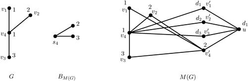To achieve this, for each $v{\prime }_i\in V\prime (G),$ first we define a set S_i containing the colors of c that can be assigned to $v{\prime }_i,$ namely, the color not assigned to any vertex in $N_G(N_G(v_i))\setminus N_G(v_i).$ Then, we consider a bipartite graph $B_M(G)$ with partite set representing the vertices with non-empty S_i and the colors of c such that an edge denotes that a particular color appears in S_i (see Figure 5). The maximum matching M_B of $B_M(G)$ gives the maximum number of vertices that can be colored using the colors of c. Using these notations, we prove the following theorem which gives an upper bound of ${\chi }^{[\#2]}(M(G))$ for any graph G.

Figure 5. The graph $B_{M(G)}$ obtained from $G=K_{1,3}$ and the exact square coloring of M(G).

Theorem 3.8.

Let M(G) denote the Mycielskian of a graph G. Then, ${\chi }^{[\#2]}(M(G))\le {\chi }^{[\#2]}(G)+n-\left|M_B\right|.$

Moreover, the bound is tight. If G is a star graph, then ${\chi }^{[\#2]}(M(K_{1,n-1}))=2n-2.$

Proof.

Let G be any graph with ${\chi }^{[\#2]}(G)=k.$ Let $c:V(G)\to [k]$ be an optimal exact square coloring of G. We define an exact square coloring, ${\varphi }_M$ of M(G) from c. For any $v{\prime }_i\in V\prime (G),$ define a set S_i as $S_i:=\{j:1\le j\le k$ and $j\ne c(v_r)\forall v_r\in N_G(N_G(v_i))\setminus N_G(v_i)\}.$ Next, consider a bipartite graph $B_{M(G)}=(X\cup Y,E_M)$ where the vertices of $X=\{s_i:1\le i\le n$ and $S_i\ne \varnothing \}$ and $Y=\{j:1\le j\le k\},$ and $E_M=\{s_{i}j:j\in S_i\}.$ Now, let M_B be a maximum matching of $B_{M(G)}$ which is easily obtained using Edwards Blossoms method for bipartite graphs. Finally, we define coloring ${\varphi }_M$ on $V(M(G))\setminus \left\{u\right\}$ using $[k]+n-\left|M_B\right|$ colors as follows: $${\varphi }_M(v)=\{\begin{array}{c}c(v),\mathrm{ }\text{if}\mathrm{ }v\in V(G),\hfill \\ j,\mathrm{ }\text{if}\mathrm{ }v=v{\prime }_i\in V\prime (G)\mathrm{ }\text{and}\mathrm{ }{s}_{i}j\in M_B\mathrm{ }\text{for}\mathrm{ }\text{some}\mathrm{ }j,\hfill \\ d_i,\mathrm{ }\text{if}\mathrm{ }v=v{\prime }_i\in V\prime (G)\mathrm{ }\text{and}\mathrm{ }{s}_{i}j\notin M_B\mathrm{ }\text{for}\mathrm{ }\text{any}\mathrm{ }j.\hfill \end{array}$$

Since $\left|M_B\right|\le k<n,$ there exist at least one vertex, say, $v{\prime }_r\in V\prime (G)$ that receives color d_r. Assign ${\varphi }_M(u)=d_r.$ To complete the theorem, we prove the following claim.

Claim 3.1.

${\varphi }_M$ is an exact square coloring of M(G) using ${\chi }^{[\#2]}(G)+n-\left|M_B\right|$ colors.

Proof.

Firstly, we prove that ${\varphi }_M$ is an exact square coloring of M(G). From Observation 3.1, we get that ${\varphi }_M$ restricted to the vertices of G is an exact square coloring as c is an exact square coloring of G. The set S_i consists of the set of colors not appearing on the set of vertices of G that are at distance 2 from $v{\prime }_i$ (namely, $N_G(N_G(v_i))\setminus N_G(v_i)\}$) and thus can be assigned to $v{\prime }_i.$ The maximum matching M_B of the bipartite graph $B_{M(G)}$ ensures that maximum number of vertices of $V\prime (G)$ are assigned colors from $[k]$ such that their color is different from the vertices of G at distance 2. The other vertices of $V\prime (G)$ are then given unique distinct colors d_i not appearing on any vertex of V(G). Thus, for every $x,y\in V\prime (G),{\varphi }_M(x)\ne {\varphi }_M(y).$ Finally, since ${\varphi }_M(u)\notin [k],{\varphi }_M$ is an exact square coloring of M(G).

Note that Observation 3.1 implies that the vertices of V(G) and $V\prime (G)$ require ${\chi }^{[\#2]}(G)$ and n colors, respectively. However, since ${\chi }^{[\#2]}(G)<n,$ some vertices of $V\prime (G)$ may use colors from $[k]$ such that the condition in Observation 3.1(iv) is not violated. The maximum matching M_B guarantees that ${\varphi }_M$ assigns colors from $[k]$ to maximum number of vertices of $V\prime (G).$ The vertex u is assigned a color distinct from the colors on the vertices of G. Thus, ${\varphi }_M$ is an exact square coloring of M(G) using ${\chi }^{[\#2]}(G)+n-\left|M_B\right|$ colors. ⋄

Therefore, ${\chi }^{[\#2]}(M(G))\le {\chi }^{[\#2]}(G)+n-\left|M_B\right|$ for any graph G.

Finally, suppose $G=K_{1,n-1}$ with $V(K_{1,n-1})=\{v_1,v_2,\dots ,v_n\}$ where $d(v_n)=n-1.$ It is clear that ${\chi }^{[\#2]}(K_{1,n-1})=n-1$ since each vertex in $\{v_1,\dots ,v_{n-1}\}$ receive distinct colors. We define an exact square coloring $\varphi$ of $K_{1,n-1}$ using n – 1 colors as follows: $\varphi (v_i)=i,1\le i\le n-1$ and $\varphi (v_n)=1.$ From above, the bipartite graph $B_{M(K_{1,n-1})}$ would be isomorphic to $K_{1,n-2}$ with $X=\left\{s_n\right\}$ and $Y=\{2,\dots ,n-1\}.$ Thus, $\left|M_B\right|=1$ and since${\chi }^{[\#2]}(M(G))\le {\chi }^{[\#2]}(G)+n-\left|M_B\right|,$ we get that ${\chi }^{[\#2]}(M(K_{1,n-1}))\le {\chi }^{[\#2]}(K_{1,n-1})+n-\left|M_B\right|=2n-2.$ Further, every pair of vertices in the set $S=\{v_1,v_2,\dots ,v_{n-1},v{\prime }_1,v{\prime }_2,\dots ,v{\prime }_{n-1}\}$ are at distance 2 and thus receive a unique color in any exact square coloring of $M(K_{1,n-1}).$ Hence, ${\chi }^{[\#2]}(M(K_{1,n-1}))\ge 2n-2.$ From the above inequalities, we conclude that ${\chi }^{[\#2]}(M(K_{1,n-1}))=2n-2.$ □

Figure 5 illustrates the exact square coloring of $M(K_{1,3})$ using six colors. Note that the constructed bipartite graph $B_{M(G)}$ has maximum matching $M_B=\{s_4,2\}$ and thus $v{\prime }_4$ can be assigned color 2.

Open Question: Characterize the graphs for which the bound in Theorem 3.8 is tight.

4. Exact square clique number of graph operations and product

In this section, we study the exact square clique number of various graph products and determine tight lower bounds. Let G and H be two graphs with $V(G)=\{g_1,g_2,\dots ,g_{n_1}\}$ and $V(H)=\{h_1,h_2,\dots ,h_{n_2}\}.$ For each $g_i\in V(G),$ let $S_G^{g_i}$ denote the set of neighbors of g_i in G that are not adjacent to each other. Similarly, for each $h_j\in V(H),$ let $S_H^{h_j}$ denote the set of neighbors of h_j in H that are not adjacent to each other. Finally, let ${\rho }_G=$ max ${}_{1\le i\le n_1}\left|S_G^{g_i}\right|$ and ${\rho }_H=$ max${}_{1\le j\le n_2}\left|S_H^{h_j}\right|.$ We will use the parameters ρ_G and ρ_H to obtain lower bound on exact square clique number of graph products.

4.1. Cartesian product of graphs

In this subsection, we give a tight lower bound on the exact square clique number of Cartesian product of two graphs.

Theorem 4.1.

Let G and H be graphs with exact square clique number ${\omega }^{[\#2]}(G)$ and ${\omega }^{[\#2]}(H)$, respectively, and the size of maximum clique $\omega (G)$ and $\omega (H)$, respectively. Then, ${\omega }^{[\#2]}(G\square H)\ge$ max $\{{\omega }^{[\#2]}(G),{\omega }^{[\#2]}(H),$ min $\{\omega (G),\omega (H)\},{\rho }_G+{\rho }_H\}.$

Moreover, the bound is tight. If $G=C_n,n>6$ and $H=P_k,k>2$, then ${\omega }^{[\#2]}(G\square H)={\rho }_G+{\rho }_H=4$, and if $G=K_n,n>2$ and H = K_k, k > 2, then ${\omega }^{[\#2]}(G\square H)=$ min $\{\omega (G),\omega (H)\}$= min {n, k}.

Proof.

Firstly, note that $d_{G\square H}((g_1,h_1),(g_2,h_2))=d_G(g_1,g_2)+d_H(h_1,h_2)$ [1]. Clearly, if $S_G=\{g\prime {\prime }_1,g\prime {\prime }_2,\dots ,g\prime {\prime }_r\}$ is an exact square clique of G, then $\{(g\prime {\prime }_1,h_1),(g\prime {\prime }_2,h_1),\dots ,(g\prime {\prime }_r,h_1)\}$ forms an exact square clique of $G\square H.$ Thus, we get that ${\omega }^{[\#2]}(G\square H)\ge {\omega }^{[\#2]}(G).$ Using similar arguments for the exact square clique of H, we get that ${\omega }^{[\#2]}(G\square H)\ge {\omega }^{[\#2]}(H).$

Next, let the maximum cliques of G and H be $C_G=\{g{\prime }_1,g{\prime }_2,\dots ,g{\prime }_s\}$ and $C_H=\{h{\prime }_1,h{\prime }_2,\dots ,h{\prime }_t\},$ respectively. Without loss of generality, assume that $s\le t.$ Consider the set $C\prime =\{(g{\prime }_1,h{\prime }_1),(g{\prime }_2,h{\prime }_2),\dots ,(g{\prime }_s,h{\prime }_s)\}.$ Note that for each pair of vertices $(g{\prime }_i,h{\prime }_i),(g{\prime }_j,h{\prime }_j)\in C\prime ,d_{G\square H}((g{\prime }_i,h{\prime }_i),(g{\prime }_j,h{\prime }_j))=d_G(g{\prime }_i,g{\prime }_j)+d_H(h{\prime }_i,h{\prime }_j)=2$ since C_G and C_H are cliques. Thus, $C\prime$ is an exact square clique of $G\square H$ and ${\omega }^{[\#2]}(G\square H)\ge$min $\{\omega (G),\omega (H)\}.$

Finally, let $g_i^{*}$ and $h_j^{*}$ be the vertices of G and H such that $\left|S_G^{g_i^{*}}\right|={\rho }_G$ and $\left|S_H^{h_j^{*}}\right|={\rho }_H,$ respectively. Let $S_G^{g_i^{*}}=\{g_1^i,g_2^i,\dots ,g_r^i\}$ and $S_H^{h_j^{*}}=\{h_1^j,h_2^j,\dots ,h_s^j\}.$ Consider the set $S=\{(g_1^i,h_j^{*}),(g_2^i,h_j^{*}),\dots ,(g_r^i,h_j^{*}),(g_i^{*},h_1^j),(g_i^{*},h_2^j),\dots ,(g_i^{*},h_s^j)\}.$ Note that any pair of vertices in S are at distance 2 from each other since $S_G^{g_i^{*}}$ and $S_H^{h_j^{*}}$ contain non-adjacent vertices having a common neighbor $g_i^{*}$ and $h_j^{*},$ respectively. Thus, S is an exact square clique of $G\square H$ and ${\omega }^{[\#2]}(G\square H)\ge {\rho }_G+{\rho }_H.$

Now, suppose that $G=C_n,n>6$ and $H=P_k,k>2$ with $V(C_n)=\{g_0,g_1,\dots ,g_{n-1}\}$ and $V(P_k)=\{h_0,h_2,\dots ,h_{k-1}\}.$ Clearly, ${\rho }_G=2$ and ${\rho }_H=2.$ Let S is the optimal exact square clique of $G\square H.$ If S contains more than one vertex of a particular copy of G, then without loss of generality, assume that $\{(g_0,h_r),(g_2,h_r)\}\in S.$ We claim that S can contain at most one vertex of another copy of G. Suppose that S contains more than one vertex of another copy of G. Then, there exists $g_i,g_j(i\ne j)$ and $h_s(s\ne r)$ such that $\{(g_i,h_s),(g_j,h_s)\}\in S.$ Since $d_{G\square H}((g_0,h_r),(g_i,h_s))=d_{G\square H}((g_2,h_r),(g_i,h_s))=2,$ we get that h_r and h_s are adjacent in H and g₀ and g₂ are adjacent to g_i in G. This implies that $g_i=g_1$ as G is a cycle. But since $d_{G\square H}((g_0,h_r),(g_j,h_s))=d_{G\square H}((g_2,h_r),(g_j,h_s))=2,$ we also get that $g_j=g_1=g_i,$ which is a contradiction. Thus, S can contain at most one vertex of another copy of G. From the above arguments, it is clear that if $(g_i,h_s)\in S$ then $g_i=g_1$ and $h_s=h_{r-1}$ or $h_s=h_{r+1}$ since H is a path graph. Thus, for any r, $1<r<k-1,S=\{(g_0,h_r),(g_2,h_r),(g_1,h_{r-1}),(g_1,h_{r+1})\}$ and ${\omega }^{[\#2]}(G\square H)=4={\rho }_G+{\rho }_H.$

Finally, suppose that $G=K_n,n>2$ and $H=K_k,k>2$ with $V(K_n)=\{g_0,g_1,\dots ,g_{n-1}\}$ and $V(K_k)=\{h_0,h_2,\dots ,h_{k-1}\}.$ Without loss of generality, assume that $n\le k.$ Then, since G is a complete graph, any exact square clique contains at most one vertex of each copy of G. Thus, $S=\{(g_0,h_0),(g_1,h_1),\dots ,(g_{n-1},h_{n-1})\}$ forms an optimal exact square clique of $G\square H$ and ${\omega }^{[\#2]}(G\square H)=n.$□

Open Question: Characterize the graphs for which the bound in Theorem 4.1 is tight.

4.2. Strong product of graphs

In this subsection, we prove a tight lower bound of exact square clique number of strong product of graphs defined in Section 3.2.

Theorem 4.2.

Let G and H be graphs with exact square clique number ${\omega }^{[\#2]}(G)$ and ${\omega }^{[\#2]}(H)$, respectively. Then, ${\omega }^{[\#2]}(G⊠H)\ge$ max $\{{\omega }^{[\#2]}(G),{\omega }^{[\#2]}(H),{\rho }_G{\rho }_H\}.$

Moreover, the bound is tight. If G and H are paths, then ${\omega }^{[\#2]}(P_2⊠P_{n_1})=2$ and ${\omega }^{[\#2]}(P_{n_1}⊠P_{n_2})=4$ for $n_1,n_2\ge 3.$

Proof.

Since for any pair of vertices of $G⊠H,d_{G⊠H}((g_1,h_1),(g_2,h_2))=$ max $\{d_G(g_1,g_2),d_H(h_1,h_2)\}$ [1], using the similar arguments as made in the proof of Theorem 4.1, we get that ${\omega }^{[\#2]}(G⊠H)\ge {\omega }^{[\#2]}(G)$ and ${\omega }^{[\#2]}(G⊠H)\ge {\omega }^{[\#2]}(H).$ Now, let $g_i^{*}$ and $h_j^{*}$ be the vertices of G and H such that $\left|S_G^{g_i^{*}}\right|={\rho }_G$ and $\left|S_H^{h_j^{*}}\right|={\rho }_H,$ respectively. Let $S_G^{g_i^{*}}=\{g_1^i,g_2^i,\dots ,g_r^i\}$ and $S_H^{h_j^{*}}=\{h_1^j,h_2^j,\dots ,h_s^j\}.$ Consider the set $S\prime =\{(g_1^i,h_1^j),(g_2^i,h_1^j),\dots ,(g_r^i,h_1^j),(g_1^i,h_2^j),(g_2^i,h_2^j),\dots ,(g_r^i,h_2^j),\dots (g_1^i,h_s^j),(g_2^i,h_s^j),\dots ,(g_r^i,h_s^j)\}.$ Note that for any pair of vertices $((g_p^i,h_l^j),(g_q^i,h_t^j))\in S\prime ,$ if p = q or l = t, then $d_{G⊠H}((g_p^i,h_l^j),(g_q^i,h_t^j))=2$ since $S_G^{g_i^{*}}$ and $S_H^{h_j^{*}}$ contain non-adjacent vertices having a common neighbor $g_i^{*}$ and $h_j^{*},$ respectively. If $p\ne q$ and $l\ne t,$ then since $d_G(g_p^i,g_q^i)=2=d_H(h_l^j,h_t^j),$ we get that $S\prime$ is an exact square clique of $G⊠H$ and ${\omega }^{[\#2]}(G⊠H)\ge {\rho }_G{\rho }_H.$

Finally, it can be easily verified that ${\omega }^{[\#2]}(P_2⊠P_{n_1})=2.$ Let $G=P_{n_1}$ and $P_{n_2}$ where $n_1,n_2\ge 3.$ Clearly, ${\rho }_G=2={\rho }_H.$ From above, we get that ${\omega }^{[\#2]}(P_{n_1}⊠P_{n_2})\ge {\rho }_G{\rho }_H=4$ for $n_1,n_2\ge 3.$ Since ${\omega }^{[\#2]}(P_{n_1}⊠P_{n_2})\le {\chi }^{[\#2]}(P_{n_1}⊠P_{n_2})$ and ${\chi }^{[\#2]}(P_{n_1}⊠P_{n_2})=4$ from Theorem 3.2, we get that ${\omega }^{[\#2]}(P_{n_1}⊠P_{n_2})\le 4.$ Thus, from both inequalities, we conclude that ${\omega }^{[\#2]}(P_{n_1}⊠P_{n_2})=4.$ □

Open Question: Characterize the graphs for which the bound in Theorem 4.2 is tight.

4.3. Lexicographic product of graphs

In this subsection, we determine the exact square clique number of the lexicographic product of two graphs.

Theorem 4.3.

Let H be a graph with clique cover number $\theta (H)$ and let G be a graph with exact square clique number ${\omega }^{[\#2]}(G)$. Then, ${\omega }^{[\#2]}(G°H)=\theta (H){\omega }^{[\#2]}(G).$

Proof.

Let $S=\{g{\prime }_1,\dots ,g{\prime }_{{\omega }^{[\#2]}(G)}\}$ be a maximum cardinality exact square clique of G. For each $i,1\le i\le {\omega }^{[\#2]}(G),$ consider the set S_i that is obtained by taking one vertex from each distinct clique of the copy of H corresponding to $g{\prime }_i.$ Let $T={\cup }_{1\le i\le {\omega }^{[\#2]}(G)}{S}_i.$ Clearly, T forms an exact square clique of $G°H$ of size $\theta (H){\omega }^{[\#2]}(G).$ Note that any exact square clique of $G°H$ contains at most $\theta (H)$ vertices of any copy of H. Next, if $S\prime$ is an exact square clique of $G°H$ such that $(g_i,h_j),(g_k,h_r)\in S\prime ,i\ne k,$ then it can be easily observed that $d_G(g_i,g_k)=2.$ Thus, T is the optimal exact square clique of $G°H$ and ${\omega }^{[\#2]}(G°H)=\theta (H){\omega }^{[\#2]}(G).$ □

4.4. Corona product of graphs

In this subsection, we determine the exact square clique number of corona product of graphs defined in Section 3.4.

Theorem 4.4.

Let H be a graph with clique cover number $\theta (H)$ and let G be a graph with exact square chromatic number ${\chi }^{[\#2]}(G)$. Then, ${\omega }^{[\#2]}(G·H)=$ max $\{{\omega }^{[\#2]}(G),\theta (H)+{\rho }_G\}.$

In particular, let H be a graph with clique cover number $\theta (H),$ then, ${\omega }^{[\#2]}(K_{1,n-1}·H)=\theta (H)+n-1$ and ${\omega }^{[\#2]}(K_n·H)=\theta (H)+1.$

Proof.

Let S be an exact square clique of maximum cardinality. Suppose S does not contain any vertex of a copy of H. Then, it is clear that S is also exact square clique of G and thus, ${\omega }^{[\#2]}(G·H)={\omega }^{[\#2]}(G).$ Now, let S contains at least one vertex of a copy of H. Then, it is it is clear that S cannot contain more than one vertex of each different copies of H. Note that if S contains two vertices of a copy of H, then they must belong to different cliques. Suppose S contains vertices of a copy of H attached to vertex $v_r\in G.$ Observe that if there exists some $v_k\in S$ such that $v_k\in V(G),$ then v_k must be adjacent to v_r. Further, for each pair of $(v_i,v_j)\in S\cup V(G),$ we have that $\{v_i,v_j\}\in S_G^{v_r}.$ Thus, if S contains at least one vertex of a copy of H, then ${\omega }^{[\#2]}(G·H)=\theta (H)+{\rho }_G.$ □

4.5. Edge corona product of graphs

In this subsection, we prove a tight lower bound of exact square clique number of edge corona product of graphs defined in Section 3.5.

Theorem 4.5.

Let G be a graph with maximum degree $\Delta (G)$ such that $G\ne K_3$. Let H be a graph with clique cover number $\theta (H)$. Then, ${\omega }^{[\#2]}(G{·}^{e}H)\ge$ max $\{{\omega }^{[\#2]}(G),\theta (H)\Delta (G)\}$. Furthermore, if G = K₃, then ${\omega }^{[\#2]}(K_3{·}^{e}H)=3\theta (H).$

Moreover, the bound is tight. If H is a graph with clique cover number $\theta (H)$ and $G=K_{1,n-1}$, then ${\omega }^{[\#2]}(K_{1,n-1}{·}^{e}H)=(n-1)\theta (H).$

Proof.

Suppose that $G\ne K_3$ contains a vertex g_r such that $d_G(g_r)=\Delta (G).$ It is clear that an optimal exact square clique of G is also an exact square clique of $G{·}^{e}H$ and thus, ${\omega }^{[\#2]}(G{·}^{e}H)\ge {\omega }^{[\#2]}(G).$ Let $N_G(g_r)=\{g_1^r,g_2^r,\dots ,g_{\Delta (G)}^r\}.$ For each edge $(g_r,g_i^r)\in E(G{·}^{e}H),1\le i\le \Delta (G),$ consider the set $S_{g_i^r}$ containing one vertex of each distinct clique of the copy of H adjacent to both g_r and $g_i^r.$ Let $S_r={\cup }_{(g_r,g_i^r)\in E(G{·}^{e}H)}{S}_{g_i^r}.$ Note that g_r is the common neighbor of any pair of vertices in S_r, implying each pair of vertices in S_r are at distance 2 from each other. Since $\left|S_r\right|=\theta (H)\Delta (G),$ we get that ${\omega }^{[\#2]}(G{·}^{e}H)\ge \theta (H)\Delta (G).$

Finally, if G = K₃, then let $E(G)=\{g_1{g}_2,g_2{g}_3,g_1{g}_3\}.$ Consider the set $S=S_{12}\cup S_{23}\cup S_{13},$ where S_ij denotes the set containing one vertex of each distinct clique of the copy of H adjacent to both g_i and g_j. It can be easily verified that S is an optimal exact square clique of $K_3{·}^{e}H$ and hence, ${\omega }^{[\#2]}(K_3{·}^{e}H)=3\theta (H).$

Finally, suppose that S is an exact square clique of $K_{1,n-1}{·}^{e}H$ of maximum cardinality. Note that if H = K_t, then we trivially get that ${\omega }^{[\#2]}(K_{1,n-1}{·}^e{K}_t)=(n-1)\theta (K_t)=n-1.$ So, we assume that $\theta (H)>1.$ If $g_i\in S,$ where g_i is any pendant vertex of $K_{1,n-1},$ then we get that $\left|S\right|\le (n-2)\theta (H),$ which is a contradiction to the above bound. Since the unique non-pendant vertex of $K_{1,n-1}$ is adjacent to each vertex in $K_{1,n-1}{·}^{e}H,$ S consists of vertices of copies of H. Thus, the set S_r is an optimal exact square clique and ${\omega }^{[\#2]}(K_{1,n-1}{·}^{e}H)=(n-1)\theta (H).$□

Open Question: Characterize the graphs for which the bound in Theorem 4.5 is tight.

4.6. Join and subdivision of a graph

In this section, we determine the exact square clique number of the graph obtained by the join and subdivision operation.

Theorem 4.6.

Let G + H denote the join of any two graphs G and H with independence number $\alpha (G)$ and $\alpha (H)$, respectively. Then, ${\omega }^{[\#2]}(G+H)$= max $\{\alpha (G),\alpha (H)\}.$

Proof.

Let S be an exact square clique of G + H. Since each vertex of G is adjacent to each vertex of H in G + H, S does not contain vertices of both G and H. Without loss of generality, let S contain vertices of G. Then, no edge in G exists between any pair of vertices of S and thus, S is an independent set in G. Hence, we get that ${\omega }^{[\#2]}(G+H)$= max $\{\alpha (G),\alpha (H)\}.$ □

Theorem 4.7.

Let G be any graph with clique number $\omega (G)$ and maximum degree $\Delta (G)$. Then, the exact square clique number of the subdivision graph S(G) is given by ${\omega }^{[\#2]}(S(G))$= max $\{\omega (G),\Delta (G)\}.$

Proof.

Suppose that S is an optimal exact square clique of S(G). Then, it is clear that if S contains a vertex $g\in G,$ then S does not contain any new vertex e_i obtained by subdividing the edge of G. Similarly, if $e_i\in S,$ then $g\notin S$ for any vertex $g\in G.$ Suppose that $g\in S.$ Then, S contains vertices that form a clique containing g in G. Now, suppose that $e_i\in S,$ then $e_j\in S$ only if e_i and e_j are both adjacent to a vertex of degree $\Delta (G).$ Thus, if S contains a vertex of G, then ${\omega }^{[\#2]}(S(G))=\omega (G),$ otherwise ${\omega }^{[\#2]}(S(G))=\Delta (G).$ □

4.7. Mycielskian of a graph

In this section, we study the exact square clique number of the Mycielskian of a graph and provide a tight lower bound.

Theorem 4.8.

Let M(G) denote the Mycielskian of a graph G with $|V(G)|=n$. Then, ${\omega }^{[\#2]}(M(G))\ge$ max $\{2{\rho }_G,n\}.$

Moreover, the bound is tight. If $G=K_{1,n-1},n>2,$ then ${\omega }^{[\#2]}(M(K_{1,n-1}))=2n-2.$

Proof.

Let M(G) denote the Mycielskian of a graph G with $|V(G)|=n.$ Let $V(M(G))=\{g_1,g_2,\dots ,g_n,$ $g{\prime }_1,g{\prime }_2,\dots ,g{\prime }_n,u\}.$ It is clear that the set $\{g{\prime }_1,g{\prime }_2,\dots ,g{\prime }_n\}$ forms an exact square clique of M(G) and thus, ${\omega }^{[\#2]}(M(G))\ge n.$ Next, let $g_i^{*}$ be the vertex of G such that $\left|S_G^{g_i^{*}}\right|={\rho }_G$ and let $S_G^{g_i^{*}}=\{g_{i,1},g_{i,2},\dots ,g_{i,r}\}.$ Consider the set $S=S_G^{g_i^{*}}\cup \{g{\prime }_{i,1},g{\prime }_{i,2},\dots ,g{\prime }_{i,r}\}.$ Since each pair of vertices in S are not adjacent and have a common neighbor $g_i^{*},$ S is an exact square clique of M(G) of size $2{\rho }_G.$ Thus, we get that ${\omega }^{[\#2]}(M(G))\ge 2{\rho }_G.$ Note that if S_G is an exact square clique of G, then $S_G\cup \left\{u\right\}$ also forms an exact square clique of size $\left|S_G\right|+1.$ But since ${\omega }^{[\#2]}(G)\le n-1,$ we get that ${\omega }^{[\#2]}(M(G))\ge n\ge {\omega }^{[\#2]}(G)+1.$

Finally, let $G=K_{1,n-1},n>2.$ Then, from above, we get that ${\omega }^{[\#2]}(M(G))\ge 2{\rho }_G=2n-2.$ Further, since ${\chi }^{[\#2]}(M(K_{1,n-1}))\ge {\omega }^{[\#2]}(M(K_{1,n-1}))$ and Theorem 3.8 implies that ${\chi }^{[\#2]}(M(K_{1,n-1}))=2n-2,$ we get that ${\omega }^{[\#2]}(M(K_{1,n-1}))\le 2n-2.$ Thus, from both inequalities, we get that ${\omega }^{[\#2]}(M(K_{1,n-1}))=2n-2.$ □

Open Question: Characterize the graphs for which the bound in Theorem 4.8 is tight.

5. Conclusion

In this article, we give tight upper bounds of the exact square chromatic number of the Cartesian product, strong product, lexicographic product, corona product, edge corona product, join and Mycielskian of graphs. These bounds are given in terms of the parameters of the component graphs. We also provide tight lower bounds of the exact square clique number of these operations. We also determine the exact values of these parameters for some specific component graphs, for example path, star graph and complete graph.

Additional information

Funding

The first author was supported by Council of Scientific and Industrial Research.

References

- Brešar, B., Gastineau, N., Klavžar, S., Togni, O. (2019). Exact distance graphs of product graphs. Graphs Combin. 35(6): 1555–1569.
- Calamoneri, T., Sinaimeri, B. (2013). L (2, 1)-labeling of oriented planar graphs. Discrete Appl. Math. 161(12): 1719–1725.
- Chang, F.-H., Chia, M.-L., Jiang, S.-A., Kuo, D., Liaw, S.-C. (2021). L (p, q)-labelings of subdivisions of graphs. Discrete Appl. Math. 291: 264–270.
- Chen, Y.-T., Chia, M.-L., Kuo, D. (2009). L (p, q)-labeling of digraphs. Discrete Appl. Math. 157(8): 1750–1759.
- Dong, W. (2020). L (p, q)-labeling of planar graphs with small girth. Discrete Appl. Math. 284: 592–601.
- Foucaud, F., Hocquard, H., Mishra, S., Narayanan, N., Naserasr, R., Sopena, E, Valicov, P. (2021). Exact square coloring of subcubic planar graphs. Discrete Appl. Math. 293: 74–89.
- Kramer, F., Kramer, H. (1969a). Ein färbungsproblem der knotenpunkte eines graphen bezüglich der distanz p. Rev. Roumaine Math. Pures Appl. 14(2): 1031–1038.
- Kramer, F., Kramer, H. (1969b). Un probleme de coloration des sommets d’un graphe. CR Acad. Sci. Paris A 268(7): 46–48.
- Lam, P. C. B., Lin, W., Wu, J. (2007). L(j, k)-labellings and circular L(j, k)-labellings of products of complete graphs. J. Comb. Optim. 14(2-3): 219–227.
- Liu, L., Wu, Q. (2020). L (1, 2)-labeling numbers on square of cycles. AKCE Int. J. Graphs Combin. 17(3): 915–919.
- Lü, D., Lin, N. (2013). L(2, 1)-labelings of the edge-path-replacement of a graph. J. Comb. Optim. 26: 385–392.
- Panda, B. S., Priyamvada (2021). Injective coloring of some subclasses of bipartite graphs and chordal graphs. Discrete Appl. Math. 291: 68–87.
- Panda, B. S., Priyamvada (2022). Complexity and algorithms for neighbor-sum-2-distinguishing {1, 3}-edge-weighting of graphs. Theor. Comput. Sci. 906: 32–51.
- Panda, B. S., Goel, P. (2011). L(2,1)-labeling of perfect elimination bipartite graphs. Discrete Appl. Math. 159(16): 1878–1888.
- Paul, S., Pal, M., Pal, A. (2013). An efficient algorithm to solve l (0, 1)-labelling problem on interval graphs. Adv. Model. Optim. 15(1): 31–43.
- Priyamvada, Panda, B. S. (2022). Exact square coloring of graphs resulting from some graph operations and products. International Conference on Graphs, Combintorics and Optimization (ICGCO), BITS Pilani, Dubai Campus.
- Sen, S. (2014). L (2, 1)-Labelings of some families of oriented planar graphs. Discuss. Math. Graph Theory 34(1): 31–48.
- Shalu, M. A., Vijayakumar, S., Yamini, S. D., Sandhya, T. P. (2018). On the algorithmic aspects of strong subcoloring. J. Comb. Optim. 35(4): 1312–1329.
- Shao, Z., Jiang, H., Vesel, A. (2018). L (2, 1)-labeling of the Cartesian and strong product of two directed cycles. Math. Found. Comput. 1(1): 49–61.
- Wu, Q., Shiu, W. C. (2017). L(j, k)-labeling numbers of square of paths. AKCE Int. J. Graphs Combin. 14(3): 307–316.