An annotated review on graph drawing and its applications

Abstract

A drawing concerns the process of generating geometric representations of relational information, usually for visualization purposes. A good drawing provides an understanding of the system to the reader, while a poor drawing may create confusion. A lot of information related to graphs and graph drawings can be stored using data structures where vertices represent entities and edges correspond to relationships among entities. In this paper, we have reviewed various studies to present the unsolved problems in the domain of graph drawing and to identify its applications in real life. By reviewing the existing approaches related to graph drawings, we found that there exist various drawing strategies that efficiently allow us to create drawings with a confined area, relatively high angular resolution, user-restrained aspect ratio, a lesser number of bends, etc. Moreover, there are several known algorithms for addressing different measures of graph drawing (such as symmetricity, spirality, rotation, etc.) but they are usually restricted to specific sub-classes of planar graphs. The present study provides readers a better understanding of the field of graph drawing and related problems.

KEYWORDS:

• Drawing
• algorithm
• graph theory
• planar graph
• crossings

1 Introduction

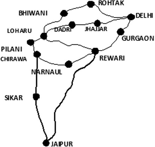
A graph G(V, E) consists of a finite and non-empty set of vertices V and a set of edges E, where each edge is a pair of elements from V. A drawing of a graph is a pictorial representation in which vertices are represented by objects such as points, circles, rectangles, boxes, while edges are represented by line segments, polylines or, a simple Jordan curve (see Figure 1). A bend in a graph drawing is a point at which an edge changes its direction. Since antiquity, this representation is used in various places such as flowcharts, route maps, computer networks, etc. A route map from Delhi to Jaipur is depicted in Figure 2, where each component (intermediary places) is drawn by a small circle and a relation among a pair of components is drawn by a line segment.

Fig. 1 Example of a drawing (where keywords of graph theory are vertices and relation between them is an edge) obtained by Vosviewer using Scopus database [135].

Fig. 2 Route map from Delhi to Jaipur.

A drawing of a graph may not be confused with the graph itself; many different layouts may correspond to the same graph. A graph is used to represent an information that can be modeled as objects and relationships among these objects while the drawing of a graph is a visualization of the abstract information depicted by the graph. Consider an example of an electronic circuit as depicted in Figure 3(a) where vertices represent its components and edges represent its interconnections. The drawing of its corresponding electronic circuit is depicted in Figure 3(b). Clearly, the graph in Figure 3(a) correctly represents the circuit, but the representation is messy, and it is difficult to comprehend and resolve. The arrangement of vertices and edges in a drawing affects comprehensibility, practicality and readability. Therefore, the main purpose of a graph drawing is to provide a better representation of a graph so that its structure is easily comprehensible and readable.

Fig. 3 Graph drawing in circuit schematics.

The flow of the paper is organized in the following way: Section 2 provides an overview of how graph drawing has evolved since its inception. Section 3 presents some glossaries associated with graph theory. Section 4 outlines the problems in the domain of graph drawing. Section 5 provides the classification and strategies used for graph drawings. Section 6 emphasizes on applications and visualization tools used for graph drawings. Section 7 presents an analysis of the study and the gaps found in the literature.

2 Historical background

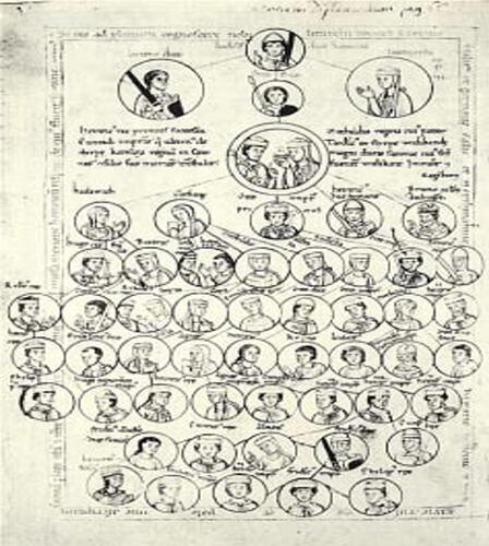
The earliest form of graph drawing was probably of Morris or Mill games [79]. The first example of Mill gameboards originated from stone sculptures in ancient Egypt are drawn in the book “Book of Games” of 13th-century, which was made under the leadership of Alfonso X (1221-1284), King of Castile and Leon [6]. Two of the drawings are depicted in Figure 4. Another ancient graph drawing is a genealogical tree. The 12th-century genealogical history of the Saxon dynasty is given in Figure 5. However, at that time nobody knew what nodes and edges represent in such drawings. The transition from early to modern graph drawing is marked by Euler in 1736 [81]. Euler introduces a problem of path tracing posed by the bridges of Königsberg, which is marked as the origin of graph theory as a subject of study. But the origin of modern graph drawing was decades later than the origin of graph theory. Graph drawing appeared more frequently and in more contexts in the late 18th and early 19th centuries. Some of the works in various fields that use graph drawings are listed below:

Fig. 4 Portrayals of 13th century Morris gameboards. The nodes are positions that game counters can occupy. The edges show how the game counters can move from node to node [121].

Fig. 5 Family tree of saxon dynasty from the Middle Ages.

1. In 1784, Haüy [102] determined the basics of crystallography. The proposed summary of crystal drawings represents a composite form of visual abstraction, which is a part of both geometric and 3D graph drawing.

2. In 1847, Listing [128] presented a path tracing problem in graphs and introduced a drawing which can be drawn with a single stroke as shown in Figure 6.

3. In 1857, Hamilton [98] designed a game using non-commutative algebraic approach and referred it as Icosian Calculas. The gameboard was a graph drawing as shown in Figure 7.

4. In 1857, Cayley [45] demonstrated his pioneering work on trees using graph drawing which can be viewed in Figure 8.

5. In 1864, Brown [43] represented molecules in the form of a graph drawing, which is an initial example of an orthogonal graph drawing.

6. In 1892, Ball [20] drew the first abstract graph drawing illustrating the Königsberg bridge problem. The graph drawing designed by him was published in his book Mathematical Recreations and Essays [19] in 1892.

Fig. 6 A graph drawing which is drawn in a single stroke given in [128].

Fig. 7 Hamiltons Icosian Game given in [32].

Fig. 8 Trees concept with labeled nodes given by Cayley in 1857.

The requirement of a large number of components in complex circuit designs in late 1960s made its hand drawing quite complicated. This problem opens the use of graph drawing in the industrial field. The domain of graph drawing to produce exquisite pictures became of interest in 1980s for presenting information on production processes and engineering. Over the last decade, advances in computational geometry, cartography, order theory, topological graph theory, and circuit design have significantly contributed to the evolution of this field.

3 Glossaries

This section presents a few terminologies of graph theory pertinent to graph drawing which are frequently used in this study. Let G be a simple connected undirected graph where n and m are the number of vertices and edges respectively and d represents the maximum degree of vertices. A graph is k-connected if it has more than k vertices and remains connected whenever less than k vertices are deleted. A graph is planar if it can be embedded in the plane without crossing of any of its two edges. A plane graph is a planar graph with a fixed plane embedding. A plane graph divides the plane into interconnected regions known as faces. The unbounded region is called external face, and all other faces except the external face are interior faces. A d-planar graphis a planar graph having a vertex of maximum degree d. A triangulated graph is a plane graph with all of its face triangles except the external face. A simple topological graph is a plane graph where vertices represent distinct points, and edges represent Jordan curves. Here, any two edges may intersect more than once, at a crossing or at the endpoint. A topological graph can be classified into k-plane or k-skew. For a k-plane graph, each edge of the graph must cross more than k times, while in a k-skew graph, the graph must become planar after the deletion of at most k edges.

4 Graph drawing problems

The problem of drawing a good graph can be considered as finding a layout of a given graph according to some measurable aesthetics. The classification of graph drawing algorithms depends on the following factors:

1. Class of graph (planar, tree, directed, etc.)

2. Graphical standard (straight-line, grid, hybrid, etc.)

3. Constraints (structural, semantic): Constraints are a part of the drawing algorithm process in order to create the final drawing. There are two purposes for applying constraints while drawing a graph. The first advantage is that it gives the possibility to the user to pre-arrange specific shapes and allows better control over the result of the drawing. Moreover, graph drawing can be a computationally expensive operation. Applying constraints can significantly expedite the process. Some common constraints include the following:

   1. Place a given vertex at the center.

   2. Place a given vertex at the boundary.

   3. Draw a sub-graph with a particular shape.

   4. Place a group of vertices together.

   5. Place a sequence of vertices on a straight line.

4. Aesthetics: The attributes which define a good drawing are known as aesthetics. Some of the qualities that determine a good drawing are as follows:

   1. Area: Minimize the area taken by a graph for its compact shape.

   2. Bends: Minimize the number of bends along an edge of a polyline drawing.

   3. Line-crossing: Minimize the number of edge crossings.

   4. Total edge length: Minimize the sum of the length of edges.

   5. Uniform edge length: Maintain the same length for each edge.

   6. Uniform density of vertices: Place each vertex at the same distance.

   7. Symmetry: Find a drawing with a maximum symmetry.

   8. Angular Resolution: Measure the sharpest angles in a graph drawing. If a graph has vertices with a high degree, then it will necessarily have a small angular resolution.

From the above list of aesthetics, we can see that some aesthetics may conflict with one another. For example, one aesthetic calls for minimizing the total edge length and the other asks for reducing the number of bends. They conflict with one another because sometimes it is preferable to include bends to have a smaller sum of the length of edges. Also, there exists a large number of possibilities for drawing a graph because while drawing a graph, we would like to consider various properties. From the informative visualization perspective, edge crossings turn out to be the major reason for reducing the readability of a graph. In contrast, planarity and symmetry in the drawing of a graph are highly desirable. Moreover, finding a drawing that satisfies two aesthetics (minimum area and minimum crossings) simultaneously, transforms the given problem transformed into a multi-objective optimization problem.

5 Classification of drawings

In this section, we introduce well-known categories of drawings. There are various graphic standards used for graph drawing. In the drawing of a graph, one has to geometrically represent the vertices and their adjacencies (edges) which can be done in various ways. In the most common types of drawing, vertices represent points or geometrical figures such as rectangles or circles, and edges represent curves such that any two edges intersect at a finite number of points. In other types of drawing, vertices represent various geometrical objects (segments, curves, polygons), whereas adjacencies represent intersections, contacts, or visibility of the objects representing vertices. Here, we present drawings where vertices are represented by points and edges represent the relationship among the vertices corresponding to an undirected planar graph. The types of drawing are described as follows:

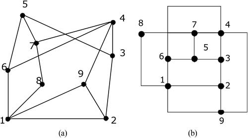
1.

Planar Drawing: A drawing in which two edges do not intersect geometrically except at their incident vertices, and the graph for which planar drawing exists is planar. It is usually easier to assimilate planar drawings than non-planar drawings (drawings with edge crossings). Hence, it is always preferable to find a planar drawing of a graph if it exists, but all graphs do not admit planar drawings. In Figure 9, a planar and a non-planar drawing of a graph is provided, and a graph for which a planar drawing does not exist.

Fig. 9 (a) A non-planar and planar drawing of a graph given by the adjacency list [(1,2), (1,3), (1,4), (2,4), (2,3), (3,4)] (b) A graph for which planar drawing does not exist.

Fig. 10 Steps for the construction of a straight-line drawing of a maximal planar graph using shift method [61].

Fig. 11 (a) A triconnected planar graph, its corresponding canonical decomposition, realizer and schynder labeling (b) A convex drawing corresponding to the triconnected graph given in (a).

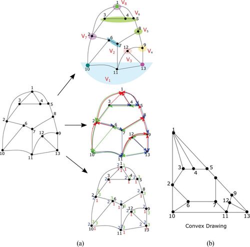
Fig. 12 (a) A plane graph G where area of each face is shown by green color and no rectangular drawing exists corresponding to it, (b) A plane graph G after adding four 2-degree vertices, (c) Rectangular draw- ing with designated corners a,b,c and d corresponding to (b), (d) An orthogonal drawing with four bends (represented by blue color) corresponding to (a), (e) An octagonal drawing corresponding to (a).

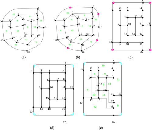
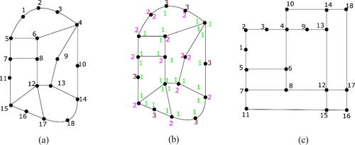
Fig. 13 Illustration of the construction of an inner rectangular drawing (a) A plane graph G (b) G with regular labelling (c) Inner rectangular drawing.

It is necessary to check the planarity of a given graph to find its planar drawing. If the graph is planar, then find its corresponding planar embedding, which is a planar drawing. We review various algorithms from the literature used for checking the planarity of a graph efficiently and computing its planar embedding. In 1930, Kuratowski [123] gave the following result for testing the planarity of a graph:

Theorem 1.

G is a planar graph if and only if it does not contain any subdivision of $K_5 or K_{3,3}$.

An equivalent result has been stated by Wagner in terms of graph minors in 1937 [172, 173]. But this characterization of the planarity of a graph does not lead to an implementable algorithm for planarity testing. Consequently, a lot of works have been done on planar graphs and some of the most relevant studies have been illustrated in Table 1. There is a lot of literature on the computation of simultaneous embedding with fixed edges, which can be achieved in polynomial time for specific classes of graphs [9, 13, 25, 64, 80, 96]. Whereas the overall problem is of unknown complexity.

Table 1 Contributions on planar drawings.

Year	Author	Contribution	Complexity of algorithm
1930	Kuratowski [123]	Characterization of planar graphs based on sub-divisions	Exponential time
1937	Wanger [172, 173]	Characterization of planar graphs based on minors	Factorial time
1961, 1963 and 1964	Auslander and Parter [17], Goldstein [91] and Bader [18]	Path addition algorithm for planarity testing	Polynomial time
1967	Lempel et al. [127]	Vertex addition algorithm for planarity testing without computing a planar embedding, if it exists	Polynomial time
1974	Hopcroft and Tarjan [105]	Improved path addition algorithm	Linear time
1976	Booth and Lueker [39]	Improved vertex addition algorithm using st-numbering algorithm and a data structure known as PQ-tree	Factorial time
1985 and 1996	Chiba et al. [50] and Mehlhorn and Mutzel [130]	Construction of a planar embedding of a given planar graph	Linear time
1999	Shih-Hsu [160]	Algorithm substitute biconnected components of the graph with a fixed embedding with single nodes called C-nodes. Performs planarity test- ing and finds planar embedding simultaneously	Linear time
1999	Boyer and Myrvold [40]	Algorithm represents embedded biconnected portions of the graph with a data structure that allows the embeddings to be flipped in constant time	Linear time
2004	Boyer et al. [41]	Method is given for planar embedding, Kuratowski subgraph isolation which is inspired by Booth-Lueker PQ tree [39] and implements vertex addition method given by Lempel Even cederbaum [127]	Linear time
2004	Giacomo et al. [66]	Planar drawing in which vertices are collinear and every edge has at most 1 bend	Linear time
2005	Giacomo et al. [65]	Planar drawing in which vertices are collinear and every edge has at most 2 bends	Linear time
2006	Fraysseix et al. [60]	Implementation of embedding algorithm in Pigale [57, 58] and simplified version of DFS-based left right planarity testing	Linear time
2008	Fraysseix and Hubert [59]	Simple planarity testing algorithm which is a new implementation of planarity algorithm based on Tremaux trees given by Hopcroft and Tarjan [104]	Linear time
2008	Haeupler et al. [95]	Vertex addition method for planarity test and implementation of Shih Hsu [160] and Boyer Myrold [40]	Linear time
2013	Schmidt and Jens [156]	Problem reduction from planar testing to construction of triconnected graphs
2015	Angelini et al. [12]	Necessary and sufficient condition for planarity testing of partially embedded graphs as well as algorithm for its implementation	Linear time
2017	Hültenschmidt et al. [106]	Planar drawing of maximal outerplanar graphs and planar 3-trees	Linear time
2018	Zeijlemaker et al. [178]	Checking planarity of any arbitrary graph (restricted to 200 vertices)	Polynomial time

2.

Polyline Drawing: A drawing in which every edge is drawn as a polygonal chain of line segments, where the common point of the successive line segments is called a bend (see Figure 14(c)). This type of drawing can have as many bends in the edges as desired. However, it may not be feasible to follow edges with greater than two or three bends physically. Polyline drawings provide great flexibility as they can approximate drawings with curved edges. When it comes to drawing a planar graph having a degree greater than four and with a good angular resolution, then polyline drawings are desirable. There are a variety of approaches which is used for planar polyline drawings with a good angular resolution, while the general approach uses a method of incremental insertion to add vertices one by one using the canonical order and continually maintaining good angular resolution qualities as well as other restrictions [47, 61]. Among all the works on polyline drawing, a few important results are as follows:

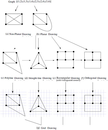
Fig. 14 Illustration of different types of drawings of complete graph K₄ (a) A non-planar drawing (b) A planar drawing (c) A polyline drawing (d) A straight-line drawing (e) A rectangular drawing which is also an orthogonal drawing (f) An orthogonal drawing which is not a rectangular drawing (g) A grid drawing of (c), (d), (e) and (f).

In 1996, Kant [112] presented a linear-time algorithm to draw planar polyline drawings for triconnected planar graphs on $(2n-6)\times (3n-9)$ grid having an angular resolution greater than 2$/d$ radians, with at most 3 bends per edge and in total, at most $5n-15$ bends. This result has been further modified and improved by Gutwenger and Mutzel [93] in 1998 by improving the grid size bound to $(2n-5)\times \left(\frac{3n}{2}-\frac{7}{2}\right)$ and by extending it to non-triconnected graphs as well. Further, in 2002 Bonichon et al. [38] presented a linear time algorithm for area optimal polyline drawings where each edge has at most one bend and has a total of at most n – 2 bends. For more results related to polyline drawings, refer to Table 2.

Table 2 Contributions on polyline drawings.

Year	Author	Contribution	Class of graphs	Complexity	Grid size	Bends	Angular
				of algorithm			resolution
1989	Tamassia and Tollis [164]	Polyline drawing	General graph	Linear time	$n\times n$	Total $2(4n+2)$ and bend along each edge is at most 4
1990	de Fraysseix, Pach, and Pollack [61]	Planar straight-line drawing using shift method (see Figure 10)	Maximal planar graph	Polynomial time	$(2n-4)\times (n-2)$
1990	Schnyder [157]	Planar straight-line drawing using realizer method	Maximal planar graph	Linear time	$(n-2)\times (n-2)$
1995	Chrobak and Payne [54]	Implemented the algorithm given in [61] using tree data structure to reduce com plexity	Maximal planar graph	Linear time	$(2n-4)\times (n-2)$
1996	Kant [112]	Planar convex grid drawing using shift method	Triconnected planar graph	Linear time	$(2n-4)\times (n-2)$
1996	Kant [112]	Algorithm to draw planar polyline drawing of a graph of n vertices on a grid with maximum degree d using canonical ordering (incremental approach)	Triconnected planar graph	Linear time	$(2n-6)\times (3n-9)$	At most 3 bend per edge and total at most 5$n-$ 15	$>\frac{2}{d}$ radians
1997	Chrobak and Kant [52]	Planar convex grid drawing using shift method	Maximal planar graph	Linear time	$(n-2)\times (n-2)$
1998	Chrobak and Nakano [53]	Planar straight-line drawing using shift method	Triangulated planar graph	Linear time	$\lfloor \frac{2}{3}(n-1)\rfloor \times 4\lfloor \frac{2}{3}(n-1)\rfloor -1$
1998	Gutwenger and Mutzel [93]	Algorithm to draw planar polyline drawing of a graph of n vertices on a grid with maximum degree d	Biconnected planar graph	Linear time	$(2n-5)\times \left(\frac{3}{2}n\text{-}\frac{7}{2}\right)$	At most 5$n-$ 15	$>\frac{2}{d}$ radians
2000	Goodrich and Wagner [92]	Algorithm to draw planar polyline drawing of a graph of n vertices on a grid with maximum degree d where every edge is a cubic bezier curve	Biconnected planar graph	Linear time	$(2n-48)\times (10n-24)$	At most 2 bend per edge	$>\frac{1}{d}$ radians
2001	Cheng et al. [47]	Algorithm to draw planar polyline drawing of a graph of n vertices on a grid with maximum degree d where edges are sequences of circular arcs	Maximal planar graph	Linear time	$30n\times 15n$	At most 1 bend per edge or at most three circular arcs	$>\frac{1}{d}$ radians
2002	Bonichon et al. [38]	Algorithm to draw polyline drawing using schnyder wood	Planar graph	Linear time	$n\text{-}\lfloor \frac{p}{2}\rfloor -1)\times (p\text{+1}),$ $p\le \frac{2n-5}{3}$	At most 1 bend per edge
2003	Duncan and Kobourov [74]	Algorithm to draw planar polyline drawing of a graph of n vertices on a grid with maximum degree d using polar coordinate representation	Planar graph	Linear time	$9n\times \frac{9n}{2}$	At most 1 bend per edge	$>\frac{1}{d}$ radians
2007	Bonichon et al. [37]	Algorithm to draw convex drawing using schnyder wood	Triconnected graph	Linear time	$\frac{3n}{4}\times \frac{3n}{4}$
2007	Dujmović et al. [73]	Straight-line drawing with at most $\frac{5n}{2}$ segments and at most 2n slopes	Triconnected graph			3 bends on the outer face	{$\frac{\pi }{ 4},\frac{\pi }{2}\frac{3\pi }{4}$}
2011	Mondal et al. [133]	Algorithm to draw straight-line drawing of a graph on a grid with a minimum area	Triconnected graph	Polynomial time	$\lfloor \frac{2n}{3}-1\rfloor \times 2\lceil \frac{n}{3}\rceil$
2012	Ackerman et al. [2]	Polyline drawing	Simple arbitrary graph			At most 2bends per edge	(0, $\frac{\pi }{2}$]${}^{\mathrm{ }}$
2013	Alam et al. [4]	Straight-line drawing	Triconnected 1-planar graph	Linear time	$(2n-2)\times (2n-3)$	Only one edge of the outer face may require 1 bend
2013	Mondal et al. [132]	Minimum segment convex drawing	Triconnected cubic planar graph	Linear time	$\left(\frac{n}{2}\text{+1}\right)\times \left(\frac{n}{2}\text{+1}\right)$
2014	Giacomo et al. [90]	Straight-line drawing	Planar graph with degree at most 3 and $n\ge 5$	Linear time	n  ×  n		$\frac{\pi }{4}$ radians
2014	Durocher et al. [75]	Polyline drawing	Maximal planar graph	Linear time		2bends per edge	$\frac{1}{d}$ radians
2015	Eades et al. [78]	Existence and construction of a straight-line drawing	At most planar graph (planar graph plus one edge), 1-skew graph	Linear time
2017	Hültenschmidt et al. [106]	Straight-line drawing that uses at most $[\frac{3n}{4}]$ segments	Tree	Linear time	${}_{n}2{\times }_{n}1.58$
2017	Bläsius et al. [35]	Straight-line drawing using approach depending on planarity-preserving force-directed algorithm [161]	Non-planar graph with a few crossings
2019	Durocher et al. [76]	Straight-line drawing using realizers with at most $\left[\frac{7n}{3}\right]$ segments 3	Planar and triangulated graph	Linear time	Polynomial grid
2019	Kindermann et al. [115]	Straight-line drawing with at most 1. $\left[\frac{3n}{4}-1\right]$ segments (a) $\left[\frac{(8n-14)}{3}\right]$ segments using schnyder realizers and orderly spanning trees 1. $\left[\frac{5n}{2}-4\right]$ segments 2. $\left[\frac{(3n-3)}{2}\right]$ segments 3. $\left[\frac{(7n-9)}{4}\right]$ segments 4. $\left[\frac{(17n-38)}{6}\right]$ segments	1. Tree 2. Triconnected planar graph 3. Maximal 4-connected planar graph 4. Biconnected outerplanar graph 5. Connected outerplanar graph 6. Connected planar graph	Linear time	1. n  ×  n2. $n\times n^2$3. $n\times n^2$4. $n\times n^2$5. $n\times n^2$6. $n\times n^2$
2020	Durocher et al. [76]	Straight-line drawing using realizers with at most $\left[\frac{7n}{3}\right]$ segments 3	Maximal planar graph	Linear time	Polynomial grid
2020	Giacomo et al. [67]	Polyline drawing which fully preserves its topology	1. 2-plane graph 2. 1-skew simple topological graph 3. k-skew simple topological graph	Linear time		1. 2 bends2. Curve complexity at most 13. Curve complexity at most 2k

• Straight-line Drawing: A polyline drawing of a graph in which each edge is drawn as a straight-line segment with no bends (see Figure 14(d)). Straight-line drawings are more accessible to follow than polyline drawings. The experimental study on human perception of graph drawings concluded that the reduction in the number of edge crossings and bends increases the understanding of graph drawings. It raises the problem of characterizing the class of graphs for which a straight-line drawing exists. This, in turn, raises the problem of devising practical algorithms for computing straight-line drawing if it exists. A classic paradigm states that there exists a planar straight-line drawing for every planar graph which is independently demonstrated by Steinitz and Rademacher [159], Wagner [171], Fary [82], and Stein [162]. Using the shift method, in 1990, Fraysseix et al. [61] proved that every planar graph where $n>=3$ vertices have a straight-line drawing on $(2n-4)\times (n-2)$ grid. Using realizer method, a similar result has been proved by Schynder [157] with an improved grid size of $(n-2)\times (n-2)$. For more work on algorithms for planar straight-line drawing on a grid, refer to Table 2.

A straight-line drawing is a monotone drawing if there exists a monotone path between every pair of vertices in some direction. There exist algorithms in the literature for constructing monotone drawings for trees, biconnected planar graphs, triconnected planar graphs, outerplanar graphs, etc. Using BFS and DFS, Angelini et al. [11] proved that a tree with n vertices admits a monotone drawing with grid size $O(n^{1.6})\times O(n^{1.6})$ and $O(n)\times O(n^2)$ respectively. It has also been shown that a biconnected planar graph also admits a monotone drawing using exponential area. Hossain and Rahman [107] presented an algorithm for computing a monotone drawing in linear time. They also proved that every connected planar graph admits a monotone drawing of grid size $O(n) \times O(n^2)$. For more work on monotone drawings, refer to [8, 14, 108, 116].

• Convex Drawing: A drawing of a planar graph in which vertices represent points and edges represent straight-line segments in such a way that the boundary of every face is a convex polygon (see Figure 14(d) and Figure 11). The boundary of a face has to pass through one of the vertices of a graph without turning. A planar graph may have a convex drawing but may not be true for another embedding. Not every biconnected graph has a convex drawing. Hence, a necessary and sufficient condition for biconnected planar graphs to have a convex drawing and its construction in linear time, if exists is given by [49]. A necessary and sufficient condition for biconnected planar graphs with the maximum degree to have an orthogonally convex drawing with no bend is given by [101]. They also propose a linear time construction for an orthogonally convex drawing, if it exists. There exists a convex drawing for every triconnected planar graph, which is not applicable for all planar graphs. The construction method of a convex planar drawing for a triconnected planar graph is presented in [49, 51, 52, 112, 167, 168]. A linear time algorithm for the construction of a convex drawing of the 4-connected graphs with four or more outer vertices is given by [131].

3.	Grid Drawing: A drawing of a graph in which every vertex and bend is located at integer grid points (see Figure 14(g)).
4.	Orthogonal Drawing: A drawing of a plane graph in which each edge is drawn as a consecutive sequence of horizontal and vertical line segments (see Figures 14(f) and 12(d)).
5.	Octagonal Drawing: An orthogonal drawing where the exterior face is drawn as a rectangle and every interior face is drawn as a rectilinear polygon having at most eight corners [148] (Figure 12(e)).

When an angular resolution is the desired criterion, then there exist many techniques for drawing a graph that accommodates it. One among them is an orthogonal drawing where edges consist of a sequence of vertical and horizontal segments. Many important results have been published on orthogonal drawings, a few of them are as follows:

There exists an orthogonal drawing of a plane graph G if every vertex of G has degree at most 4. Conversely, a plane graph with every vertex of degree at most 4 has an orthogonal drawing but it may require bends. Hence, there have been a lot of studies to minimize the number of bends in an orthogonal drawing, out of which some of the important results are as follows: Nakano [134] presented a linear time algorithm for bend optimal orthogonal drawings for biconnected cubic planar graphs. Rahman et al. [150] presented the minimum number of bends required in an orthogonal drawing for triconnected cubic planar graphs which is $b(G)+4-k$ where k is the number of corner 3-legged cycles, $b(G) ={\sum }_{i=1}^{l}bc(C_i)$, $bc(C_i)$ is a bend count corresponding to C_i and C_i is a maximal 3-legged cycle in G. He also presented a necessary and sufficient condition to check the existence of an orthogonal drawing without bends corresponding to a 3-plane graph (refer to [153]). More results and related literature are given in Table 3.

Table 3 Contributions on orthogonal drawings.

Year	Author	Contribution	Class of graphs	Complexity	Area	Bends
				of algorithm
1980	Leiserson [126]	Orthogonal drawing	4-outer planar graph	Linear time	O(nlog${}^{2}n)$
1981	Valiant [170]	Orthogonal drawing	4-planar graph		O(nlog${}^{2}n)$
1984	Leighton [125]	Orthogonal drawing	4-planar graph		O(nlogn)
1987	Tamassia [165]	Orthogonal drawing with minimum bends using network flow	4-planar graph	$O(n^2$logn)		At most $3n+2$
1989	Tamassia and Tollis [164]	Orthogonal drawing using visibility representation	4-planar graph	$O(n^2$logn)		At most $2n+1$ and two edges have more than 2 bends if biconnected else $2(4n+2)$ and no edge with more than 4 bend
1993	Formann et al. [85]	Determining whether an orthogonal drawing with no bend exists	4-planar graph	NP-Hard
1995	Schaffter [155]	Constructing embedding of a 4-plane graph on a rectangular grid	4-planar graph	$O(n^2)$		At most 2n and 2 bend per edge
1997	Garg and Tamassia [88]	Minimum bend orthogonal drawing of a 4-planar graph	4-planar graph	$\mathrm{(}\text{HTML translation failed}\mathrm{)}$
1998	Biedl and Kant [30]	Constructing an orthogonal drawing of a connected graph	Planar and non-planar graph	Linear time	At most $O(n^2)$	At most $2n+4$ and each edge has at most 2 bends
1998	Papakostas and Tollis [143]	Construction of an orthogonal drawing	3-planar graph and non-pla nar connected graph with degree at most 4	Linear time	At most 14$n^2$ and $0.76n^2$	At most $\lceil \frac{n}{2}\rceil +3$ and $2n+2$ respectively
1998	Battista et al. [63]	Orthogonal drawing with minimum bends along edges using spirality	3-planar graph	$O(n^5$logn)
2000	Bertolazzi et al. [27]	Computing an orthogonal drawing with minimum bends using branch and bound approach	Biconnected planar graph	Linear time
2002	Rahman et al. [146]	Necessary and sufficient condition for 3-plane graph if an orthogonal drawing without bend exists	3-planar graph	Linear time
2003	Rahman and Nishizeki [150]	Minimum bend orthogonal drawing for 3-planar graph	3-planar graphs	Linear time
2011	Blasius et al. [34]	Orthogonal drawing with rotation as a flexibility measure	4-planar graph	Linear time
2012	Cornelsen and Karrenbauer [55]	Minimizing the bend number in the orthogonal drawing of a plane graph	4-planar graph	$O\left(n^{\frac{5}{2}}\right)$		At most 1 bend per edge
2012	Bekos et al. [26]	Smooth orthogonal drawing of a plane graph	Biconnected 4-planar graph			3 bend per edge
2014	Alam et al. [3]	Smooth orthogonal drawing of a plane graph with low edge complexity	4-planar graph		Polynomial area	2 bend per edge
2015	Biedl and Schmidt [31]	Area can be reduced in case of triconnected graph	Triconnected planar graph	Linear time	$0.56n^2$	$(2-ϵ)$, where $ϵ\mathrm{>}0$
2017	Chang and Yen [46]	An faster algorithm for bend minimum orthogonal drawing	4-planar graph	$O\left(n^{\frac{17}{7}}\right)$
2018	Didimo et al. [71]	An algorithm for computing orthogonal drawing in a variable embedding setting with minimum bends	3-planar graph	$O(n^2)$
2018	Jünger et al. [109]	A new compact model and an algorithm for orthogonal drawing that allows altering in shape by re ducing total edge length and area at the expense of additional bends	4-planar graph	Polynomial time
2018	Bhatia et al. [29]	Orthogonal drawing with minimum bend number corresponding to a given graph	Triconnected cubic planar graph	Linear time		b + 3k
2019	Hasan and Rahman [101]	Existence and construction of an orthogonal draw ing with no bend corresponding to a given graph, if exists	Biconnected planar graph with maximum degree 3	Linear time
2020	Didimo et al. [72]	Orthogonal drawing corresponding to a given graph with minimum bend number	3-planar graph	Linear time
2020	Bekos et al. [23]	An algorithm for testing whether a turn regular orthogonal drawing exists	Biconnected plane graph		Polynomial time	No bends
2020	Angelini et al. [15]	Existence of extended partial orthogonal drawings	Planar graph		Linear time	O(|V(H)|) bends per edge
2021	Niedermann and Rutter [136]	An integer-linear program (ILP) for computing ortho-radial representations with a given embedding	Planar graph with maximum degree 4			Bend free
2022	Didimo et al. [69]	Computing orthogonal drawing with minimum number of bends	Plane series-parallel 4-graph	Linear time
(Continued)

1. Rectangular Drawing: A drawing of a plane graph in which each vertex represents a point and edges connecting them represents vertical and/or horizontal line segments with no crossings. All faces of the drawing are represented by rectangles (see Figures 14(e) and 12(c)). Since, all graphs do not have rectangular drawings, in 1984, Thomassen [36] provided a necessary and sufficient condition for a plane graph with exactly four vertices of degree 2 to have a rectangular drawing. Further, Rahman et al. [149] proved that a plane graph with a maximum degree 4 has a rectangular drawing if and only if four of its vertices have degree 2 and they lie on its outer boundary. In 2004, Rahman et al. [152] gave a linear time algorithm for checking the existence of a rectangular drawing for planar graphs having maximum degree 3. Miura et al. [131] proved that a plane graph G with maximum degree four has a rectangular drawing if and only if the decision graph G_d of G has a perfect matching. It can be found in $O(n^{1.5})$ time, if it exists. For further results on rectangular drawings, refer to Table 4. Rectangular drawings have applications in VLSI and architectural design processes [152]. The input of a floor planning problem in VLSI circuit designing is a plane graph where each functional entity of a circuit is a module represented by a vertex, and interconnection between modules is a wire represented by an edge. The output of the design is required as a partition of a rectangular chip area into smaller rectangles representing modules. If two vertices are adjacent, then the corresponding rectangles must share a common boundary.

Table 4 Contributions on rectangular drawings for planar graphs with maximum degree d.

Year	Author	Contribution	Class of graphs	Complexity of algorithm
1984	Thomassen [36]	Necessary and sufficient condition for the existence of a rectangular drawing when 4 outer vertices of degree 2 are designated as corners	Planar graph with maximum degree at most 3
1984	Koźmiński and Kinnen [120]	Necessary and sufficient condition for the existence of a rectangular drawing and its construction if exists	Inner triangulated planar graph	$O(n^2)$
1988	Bhasker and Sahni [28]	Construction of a rectangular drawing	Inner triangulated planar graph	Linear time
1990	Lai and Leinwand [124]	Reduction of the problem of finding a rectangular drawing to finding a perfect matching of new bipartite graph con structed from its corresponding graph	Planar graph of maximum degree at most 3	$O(n^{2.5})$
1997	Kant and He [111]	Algorithm that computes a rectangular drawing from regular edge labelling	4-connected triangulated graph	Linear time
1998	Rahman et al. [149]	Rectangular drawings with designated corners	Planar graph of maximum degree at most 3	Linear time
2002 and 2004	Rahman et al. and Nishizeki and Rahman [151], [137]	Necessary and sufficient condition for the existence of a rectangular drawing while choosing a few outer vertices as corners	Planar graph of maximum degree at most 3	Linear time
2004	Rahman et al. [152]	Existence and construction of rectangular drawings	Planar graph of maximum degree at most 3	Linear time
2006	Miura et al. [131]	Rectangular drawing exists if and only if its constructed bipartite graph has a perfect matching	Planar graph of maximum degree at most 4	$O(n^{1.5}$/logn)
2022	Alegria et al. [5]	Existence of an unit-length rectangular drawing depending on outer face	Planar graph	$O(n^2/lo{g}^{3}n)$

In the VLSI circuit design, since each module has some specific physical area, the area of the circuit needs to be optimized within the given space. In area optimization, there may be some cases where rectangular drawings are not useful due to the insufficiency of satisfying the prescribed area. In such cases, it is preferred to draw each inner face of the drawing as a rectilinear polygon. An abundance of literature is available on rectilinear drawings of plane graphs with prescribed face areas [113, 114, 148].

In architectural floor planning, a similar problem arises. The user has some specific preferences while building a house; for example, a living room must be adjacent to a bedroom. According to the users preferences, the problem can be modeled using a plane graph, where every vertex represents a room, and the edge represents the required adjacency between the rooms. A feasible solution for the floor planning problem is a rectangular drawing of a plane graph which is a floor plan. It can be noted here that the exterior face of the VLSI circuit or architectural floor plan may not always be rectangular, i.e., it may be a rectilinear polygon of the shape of say L, T, Z, etc. Such kind of a drawing is known as inner rectangular drawing where every inner face is a rectangle; however, the exterior face is rectilinear (see Figure 13(c)).

Note 1. On Non-Planar graphs: This study focuses on different types of drawings for planar graphs whereas researchers have recently shifted their interest to geometric representations of non-planar graphs as most of the real-world networks, for example social networks, are non-planar. Directly moving from planar to non-planar is very challenging hence the term beyond planarity has been introduced. Beyond planarity means non-planar graphs with specific types of crossings, for example k-planar graphs, k-quasi-planar graphs, RAC graphs, fan-crossing-free graphs etc. For a detailed work related to these graphs, refer to [1, 10, 24, 44, 68, 70, 103, 138].

5.1 Drawing strategies

This section elaborates few of the most effective well-known methods that have been developed for drawing general graphs.

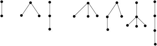
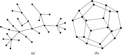
1. Force directed graph drawing method: This method of a graph drawing is used to position the vertices of a graph in 2D or 3D so that all the edges are of approximately the same length with a few edge crossings (see Figure 15). The nodes of the graph represent the bodies of the system on which forces are applied. These forces have a natural analogy of either attraction or repulsion. In any force graph drawing, the edges of the graph can be modeled as an attractive force while the nodes as repulsive forces which can be used to simulate the motion of edges and nodes or to minimize the energy layout of the nodes. In this method, the position of the initial vertex changes continuously depending on the movement of other vertices due to a system of forces based on the iterative optimization of their relative positions. This method can also simulate unnatural forces acting on the system bodies. These forces are used to obtain drawings with small edge lengths and all pairs of vertices well separated. Force directed graph drawing methods have a prolonged history. In the 1960s and 1970s [84, 145], force directed graph drawing methods were used in VLSI layouts. But it renewed its interest in 1990s [56, 100]. The first” force directed” graph drawing method is given by Tutte [168] which uses barycentric representations for obtaining straight-line drawing with no edge crossing corresponding to a triconnected planar graph. He also guarantees that the obtained drawing is with no edge crossings. But this approach is limited to small graphs for vertices less than 100 (refer to [77]) and it produces poor drawings. Several other approaches for force directed graph drawing methods came in the late 1990s which can be applied to large graphs with vertices greater than hundred of thousands [86, 87, 94, 99]. Simplicity and intuitivity of this method appeal to researchers from many different fields [42, 48, 83, 118, 119, 122, 141, 176].

Fig. 15 Examples of Force directed graph drawings (a) Structure of a tree (b) Dodecahedron (20 vertices).

Advantages:

• This method provides results based on quality measures such as uniform vertex distribution, uniform edge length, and symmetry.

• The method is intuitive as it relies on natural analogies of common objects, such as springs, which makes it easy to anticipate and understand.

• The drawings produced by this method are often symmetric.

• In a drawing, if any vertex needs to be placed far from any other vertex, then this can be done by increasing the force on connecting edge between them.

• The method is simple, interactive, and easily extendable to 3D.

• Heuristic algorithms can be easily added to this method.

Disadvantages:

1. High running time: This approach has a polynomial running time (O(n ${}^3$)), where n is the number of vertices of the input graph.

2. Poor local Minima: The output of this method is a graph with minimal energy, especially when total energy is only a local minimum. In many cases, a local minimum is worse than a global minimum because it converts into a poor-quality drawing. When the number of vertices of the graph increases, the problem of poor local minima becomes more significant.

3. General graphs: This approach is preferred when you draw general graphs and have no domain-specific information (or any other topological information) about them. It is difficult to obtain orthogonal and polyline drawings with this approach.

4. Topology-Shape-Metrics: A three-step process is required for this method. The output of this approach is an orthogonal drawing that is used in electrical engineering and other applications [21, 117, 139]. The aesthetic measures of this approach are minimum crossing, area, and edge length. An orthogonal drawing is described by three properties, defined in terms of topology, shape, and metrics which are described below:

   1. Topology: Two orthogonal drawings are topologically equal if one of them can be obtained by continuous deformation of other without altering the sequence of edges which contours the faces of the drawing.

   2. Shape: Two orthogonal drawings are of the same shape if the drawings have the same topology. One drawing can be obtained from other by only varying the length of the edges without changing the angles between edges.

   3. Metrics: Two orthogonal drawings are of the same metric if the drawings are congruent and can be converted into each other by translation and/or rotation.

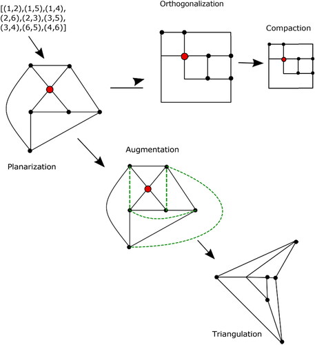
The Topology-Shape-Metrics algorithm can be explained in the following three steps based on the mentioned properties (see Figure 16):

1. Planarization: In planarization, the mathematical representation of a graph is converted into a 2D drawing to obtain the graph’s topology. In this process, the number of edge crossings is optimized to a minimum. For each edge crossing, a dummy vertex needs to be introduced in the drawn planarized graph.

2. Orthogonalization: In orthogonalization, the vertices are aligned, and bends are shaped at the right angle. In the process, the topology of the graph must remain unchanged while minimizing the number of bends.

3. Compaction: In compaction, dummy vertices are eliminated, and the area of the graph is optimized to a minimum by reducing the edge length. The output of this process is metrics.

Fig. 16 Steps for Topology-Shape-Metrics and Augmentation approach.

Advantages:

• This approach is rich in a variety of aesthetic measures such as minimum edge crossing, edge length, and minimum area, etc.

• This approach has linear run time for planar graphs whereas polynomial for non-planar graphs.

• This approach is simple and comprehensible.

• This approach may lead to entirely different drawings.

Disadvantages:

• Not applicable for graphs with vertices of degree more than 4.

3. Augmentation: This graph drawing approach is also a three-step process [22]. Straight-line or polyline drawing with no bends is obtained from this process. Aesthetic measures in this approach are minimum crossing due to the straight-line approach to the triangulation.

This method also requires a three-step process which is described as follows (see Figure 16):

1. Planarization: This step is described by a planar embedding of a graph if it exists. Otherwise, try to keep a minimum edge crossing, then to planarize, a dummy vertex is inserted for every edge crossing. This step is similar to that described in the Topology-Shape-Metric approach.

2. Augmentation: In this step, a maximal planar graph is obtained by adding dummy edges.

3. Triangulation: In this step, the final graph is obtained from the previous step using the geometric properties of the triangles and by eliminating dummy vertices and edges.

Advantages:

• This approach is applicable to graphs of a higher degree.

• This approach results in a straight-line drawing.

• This approach opens the way for other aesthetic measures such as angular resolution.

Disadvantages:

• This approach is based on a single aesthetic criterion.

• Not applicable to polyline drawings with bends.

6 Applications of graph drawing

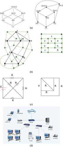
Graph drawing has diverse applications in different fields. Some of the real-life applications (see Figure 17) are as follows:

1. Architecture: In the initial step of architecture floor planning, the user has certain specifications to build a house. The graph drawing makes it possible to draw an initial outline of the plan according to the preferences of the user who establishes the relations and connections between the different parts of the plan [154, 169].

2. VLSI Circuits: Graph drawing is used to design VLSI circuits [110].

3. Software Engineering: Applications related to large-scale object-oriented software systems to support maintenance and re-engineering processes can be visualized better using graph drawings [163].

4. Sociograms: Drawings depicting social networks (refer to Chapter 25 of [166] and [158]).

5. Hasse Diagrams: Drawings specialized for partial orders [62].

6. State Diagrams: Drawings that gave the graphical illustrations of finite state automaton [7].

7. Computer Network Schematics: Computer networks can be illustrated using drawings where vertices and edges in the drawing represent the nodes and connections between various systems respectively (refer to chapter 26 of [166]).

8. Flow Charts: Flow charts can be represented with drawings where nodes and edges show the steps of an algorithm and the flow of control between steps respectively [174].

9. Bioinformatics: In drug design, drawings are being used to represent the 2D form of molecular structures or in displaying RNA structures (refer to chapter 20 of [166]).

Fig. 17 Examples of some applications of graph drawing (a) A Hasse diagram of the subsets of a 3-element set and its more readable drawing (b) A plane graph (represented by black lines) is the given adjacency requirement for designing problem and orthogonal drawing of its corresponding dual (represented by green lines) is a floor plan layout which is useful in both architecture and VLSI chip design (c) An electronic circuit and its corresponding orthogonal drawing (d) Computer networks.

6.1 Visualization tools

There are various tools for visualizing the drawings of a graph such as

1. BioFabric [33]: It is an open source software which is used to visualize large networks by node-link diagrams.

2. Cytoscape [140]: It is an open source software used to view the molecular interaction networks.

3. Graph-tool [144]: It is a free Python module which is used for the statistical analysis of graphs and their manipulations.

4. Mathematica [175]: It is a computational tool for the visualization and analysis of 2D and 3D graphs.

5. NetworkX [97]: It is a Python package used to study of structures, dynamics and complex networks. It is also used to create or manipulate data structures in graph drawing.

6. Tulip [16]: It is an open source tool used for data visualization.

7. yEd [177]: It is a multi-document desktop application which is used to generate drawings manually or by importing external files for the data or graph analysis.

8. Graphviz [129]: It is an open-source software which is used for graph and network visualization.

9. Pigale [57]: It is an open source software basically used in the research oriented to theoretical study of graphs. It is a C $++$ algorithm library which is used for planar graphs.

10. Gephi [89]: It is an open source software for visualization, manipulation and exploration for all kinds of graphs and networks. It is written in Java on the NetBeans platform.

11. Pajek [142]: Pajek means “spider” in slovenian language. It is a program for visualization and analysis of large networks in windows.

7 Discussion and open problems

This paper describes the graph drawing problem and discusses a lot of its qualitative and algorithmic aspects. In particular, we characterize the graph drawing problem and classify the types of drawing which are used for an undirected simple graph. In this study, we have presented the work which is reviewed in a progressive manner for a better understanding. Also, we briefly review some of the recent findings and outlined some emerging research directions. The review includes some of the traditional approaches used for the drawing of graphs mentioned in the drawing strategies section. One of the important parts of a graph drawing is planar drawing from which the graph drawing problem is initiated. Planar drawings are more efficient at understanding the data and increase its readability. In this direction, the construction of an acceptable drawing for the graphs for which planar drawing doesn’t exist is still unanswered. Further, there are various types of aesthetics which require to define a good drawing. Every drawing type has its aesthetic quality, for example planar drawing primarily includes line crossing and polyline drawings feature bends for a good drawing. We analyze from this study that most of the work which is done for any type of drawing either considers a specific type of class of graphs or any aesthetic. There is no work on the drawings which is generally applied to any arbitrary graph and provides the required drawing, if it exists. Despite the profusion of literature on graph drawing, several theoretical and practical problems are still open, which need to be addressed. We strived to include a few of the open problems that are motivated by the topics of general interest in this field. A list of a few of the most promising directions for further research is mentioned below.

• Practical implementation: Implementations of some of the algorithms are used in empirical work but are limited to specific graphs on a small scale (with vertices less than 100), such as an algorithm for floor planning, chip designing, etc. The algorithmic behavior of general graphs cannot be simulated from theoretical analysis of a specific class of graphs such as d-planar, biconnected, etc. Therefore, it is required to perform extensive practical study for large graphs to increase their visualization in real-time applications.

• Performance Criterion: In planarization, there is no specific performance criterion for any heuristic. However, for the design of VLSI circuits or aesthetic graph drawing, definite heuristic approaches are required.

• Planarity Testing: There are algorithms (path addition, vertex addition) for planarity testing, which are achievable in linear time. As the algorithms are complex and challenging to implement, it limits their use in practical systems. Therefore, for testing and constructing the planar representation of a graph efficiently, significant efforts are required.

• 3D Drawings: Based on the literature, authors believe that the development of practical algorithms for drawings in 3D space would be thought-provoking.

• Complexity:

  1. It is known that the problem of checking the planarity of any arbitrary graph and checking whether it admits a planar drawing was done first exponentially [123] and then reduced in polynomial time [178]. Is it possible that its implementation can be further reduced to linear time?

  2. Construction of a polyline drawing corresponding to any arbitrary graph with at most four bends per edge can be done in linear time [164]. Further, it can be done with at most two bends per edge [2]. Is it possible that it can be constructed with less than at most two bends per edge and in linear time?

  3. It can be seen that the construction of an orthogonal drawing corresponding to 4-planar graphs can be done in polynomial time [46, 55, 88, 164, 165]. Most efficient algorithm till now has time complexity $O\left(n^{\frac{17}{7}}\right)$. Can we compute bend minimum orthogonal drawing for 4-planar graphs more efficiently?

  4. Is it possible to construct rectangular drawing corresponding to 4-planar graphs in linear time?

• Bend Minimization in Orthogonal Drawings: The problem of minimization of bends in planar orthogonal drawings is NP-hard in general but can be done in polynomial time for a fixed planar embedding. The minimum number of bends corresponding to several classes of graphs (biconnected planar graphs, 3-planar, etc.) can be obtained in linear time. Based on this study, we suggest a few research problems for future directions related to the improvement of bend minimum orthogonal drawing as follows:

  1. It is still unknown that for every possible choice of exterior face, is there any linear time algorithm which gives minimum bends in an orthogonal drawing corresponding to the planar graph with a fixed embedding except for 3-plane graphs?

  2. The bend number in orthogonal drawings of the same graph with different planar embeddings are not the same. Hence, finding a planar embedding of a plane graph which gives the bend minimum orthogonal drawing is important (see Figure 18).

  3. It is still unknown that for a 4-plane graph with fixed embedding, is there any linear time algorithm which gives bend minimum orthogonal drawing.

  4. Battista et al. [22] work for a 3-plane graph and provides bend minimum orthogonal drawing in $O(n^{5}l\mathit{ogn})$ time but in general, the problem of finding an embedding of a plane graph which corresponds to bend minimum orthogonal drawing is NP-complete.

• No Bend Orthogonal Drawings: It can be easily seen that there is work on no bend orthogonal drawing for a biconnected planar graph with maximum degree 3 [153] and subdivision of a triconnected cubic planar graph [147] but it is still unanswered for 4-planar graphs. Establishing a necessary and sufficient to obtain no bend orthogonal drawing for a 4-planar graph is still open (see Figure 19).

• Enumeration of Drawings: In the literature, there are algorithms that compute only one drawing of a given graph with a fixed embedding satisfying a specific aesthetic criterion. However, there may be more than one drawing corresponding to the same graph that meets the same criteria (see Figure 20).

• Angular Resolution in Straight-line Drawings: Achieving optimal angular resolution is NP-hard. Hence, is it possible to compute optimal angular resolution approximation efficiently? There are special classes of planar graphs for which good angular resolution can be obtained (i.e., $\rho =O\left(\frac{1}{d^k}\right)$ where k is a small constant). Can it be achievable for all planar graphs?

• Symmetricity in Drawings: Symmetricity is an aesthetic criterion which is rarely considered in the discussed drawings. We believe that including symmetricity in drawings increases the impact of the drawing by making it more efficient and readable.

Fig. 18 Example for bend minimization problem (a) A triconnected cubic planar graph with exterior face of length 3 and its orthogonal drawing with minimum number of bends according to [29, 146] (b) Same graph as in part (a) and its corresponding orthogonal drawing with lesser number of bends in comparison to (a).

Fig. 19 (a) A 4-plane graph (b) An orthogonal drawing corresponding to (a) with no bends.

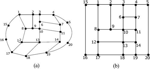
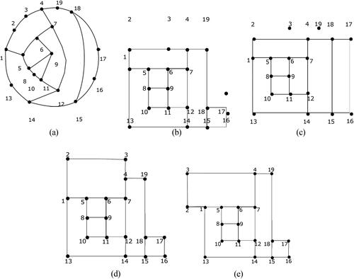
Fig. 20 Enumeration of orthogonal drawings (a) A 3-plane graph G (b)–(e) Different orthogonal drawings of (a) having same characterstics and different shapes.

References

- Ackerman, E. (2014). A note on 1-planar graphs. Discrete Appl. Math. 175: 104–108.
- Ackerman, E., Fulek, R., Tóth, C. D. (2012). Graphs that admit polyline drawings with few crossing angles. SIAM J. Discrete Math. 26(1): 305–320.
- Alam, M. J., Bekos, M. A., Kaufmann, M., Kindermann, P., Kobourov, S. G., Wolff, A. (2014). Smooth orthogonal drawings of planar graphs. In: Latin American Symposium on Theoretical Informatics, Berlin, Heidelberg: Springer, pp. 144–155.
- Alam, M., Brandenburg, F. J., Kobourov, S. G. (2013). Straight-line grid drawings of 3-connected 1-planar graphs In: International Symposium on Graph Drawing, Cham: Springer, pp. 83–94.
- Alegria, C., Da Lozzo, G., Di Battista, G., Frati, F., Grosso, F., Patrignani, M. (2022). Unit-length rectangular drawings of graphs. arXiv preprint arXiv:2208.14142.
- Alfonso, X. (1843). King of Castile and León Libros del ajedrez, dados y tablas.
- Anderson, J. A. (2006). Automata Theory with Modern Applications. Cambridge: Cambridge University Press.
- Angelini, P. (2017). Monotone drawings of graphs with few directions. Inf. Process. Lett. 120: 16–22.
- Angelini, P., Battista, G. D., Frati, F. (2013). Simultaneous embedding of embedded planar graphs. Int. J. Comput. Geom. Appl. 23(02): 93–126.
- Angelini, P., Bekos, M. A., Kaufmann, M., Pfister, M., Ueckerdt, T. (2018). Beyond-planarity: Turán-type results for non-planar bipartite graphs. In: 29th International Symposium on Algorithms and Computation (ISAAC 2018). Schloss Dagstuhl-Leibniz-Zentrum fuer Informatik.
- Angelini, P., Colasante, E., Battista, G. D., Frati, F., Patrignani, M. (2010). Monotone drawings of graphs. In: International Symposium on Graph Drawing, Berlin, Heidelberg: Springer, pp. 13–24.
- Angelini, P., Di Battista, G., Frati, F., Jelínek, V., Kratochvíl, J., Patrignani, M., Rutter, I. (2015). Testing planarity of partially embedded graphs. ACM Trans. Algorithms 11(4): 1–42.
- Angelini, P., Di Battista, G., Frati, F., Patrignani, M., Rutter, I. (2012). Testing the simultaneous embeddability of two graphs whose intersection is a biconnected or a connected graph. J. Discrete Algorithms 14: 150–172.
- Angelini, P., Didimo, W., Kobourov, S., Mchedlidze, T., Roselli, V., Symvonis, A., Wismath, S. (2015). Monotone drawings of graphs with fixed embedding. Algorithmica 71(2): 233–257.
- Angelini, P., Rutter, I., Sandhya, T. P. (2020). Extending partial orthogonal drawings In: International Symposium on Graph Drawing and Network Visualization, Cham: Springer, pp. 265–278.
- Auber, D., Mary, P. (2007). Tulip: Data Visualization Software, Version 5.6.3. https://tulip.labri.fr/TulipDrupal/
- Auslander, L., Parter, S. V. (1961). On imbedding graphs in the sphere. Indiana Univ. Math. J. 10(3): 517–523.
- Bader, W. (1964). Das topologische Problem der gedruckten Schaltung und seine Lösung. Archiv f Elektrotechnik 49(1): 2–12.
- Ball, W. R. (1893). Mathematical recreations and essays. Bull. des Sci. Math. 17: 105–107.
- Ball, W. W. R. (1914). Mathematical Recreations and Essays. London: Macmillan.
- Barth, L., Niedermann, B., Rutter, I., Wolf, M. (2017). Towards a topology-shape-metrics framework for orthoradial drawings. In: 33rd International Symposium on Computational Geometry (SoCG 2017), Schloss Dagstuhl-Leibniz-Zentrum fuer Informatik.
- Battista, G. D., Eades, P., Tamassia, R., Tollis, I. G. (1998). Graph Drawing: Algorithms for the Visualization of Graphs. Hoboken, NJ: Prentice Hall PTR.
- Bekos, M. A., Binucci, C., Battista, G. D., Didimo, W., Gronemann, M., Klein, K., Patrignani, M., Rutter, I. (2020). On turn-regular orthogonal representations. In: International Symposium on Graph Drawing and Network Visualization, Cham: Springer, pp. 250–264.
- Bekos, M. A., Didimo, W., Liotta, G., Mehrabi, S., Montecchiani, F. (2017). On RAC drawings of 1-planar graphs. Theoret. Comput. Sci. 689: 48–57.
- Bekos, M. A., Dijk, T. C. V., Kindermann, P., Wolff, A. (2015). Simultaneous drawing of planar graphs with right-angle crossings and few bends In: International Workshop on Algorithms and Computation, Cham: Springer, pp. 222–233.
- Bekos, M. A., Kaufmann, M., Kobourov, S. G., Symvonis, A. (2012). Smooth orthogonal layouts. In: International Symposium on Graph Drawing, Berlin, Heidelberg: Springer, pp. 150–161.
- Bertolazzi, P., Di Battista, G., Didimo, W. (2000). Computing orthogonal drawings with the minimum number of bends. IEEE Trans. Comput. 49(8): 826–840.
- Bhasker, J., Sahni, S. (1988). A linear algorithm to find a rectangular dual of a planar triangulated graph. Algorithmica 3(1–4): 247–278.
- Bhatia, S., Lad, K., Kumar, R. (2018). Bend-optimal orthogonal drawings of triconnected plane graphs. AKCE Int. J. Graphs Comb. 15(2): 168–173.
- Biedl, T., Kant, G. (1998). A better heuristic for orthogonal graph drawings. Comput. Geom. 9(3): 159–180.
- Biedl, T., Schmidt, J. M. (2015). Small-area orthogonal drawings of 3-connected graphs. In: International Symposium on Graph Drawing, Cham: Springer, pp. 153–165.
- Biggs, N., Lloyd, E. K., Wilson, R. J. (1986). Graph Theory. Oxford: Oxford University Press, pp. 1736–1936.
- Biofabric, Version 2 Beta Release 2 (2019). Available at: http://www.biofabric.org/
- Bläsius, T., Krug, M., Rutter, I., Wagner, D. (2010). Orthogonal graph drawing with flexibility constraints In: International Symposium on Graph Drawing, Berlin, Heidelberg: Springer, pp. 92–104.
- Bläsius, T., Radermacher, M., Rutter, I. (2017). How to draw a planarization. In: International Conference on Current Trends in Theory and Practice of Informatics, Cham: Springer, pp. 295–308.
- Bondy, J. A., Murty, U. S., eds. (1984). Progress in Graph Theory, Vol. 2. Toronto; Orlando: Academic Press.
- Bonichon, N., Felsner, S., Mosbah, M. (2007). Convex drawings of 3-connected plane graphs. Algorithmica 47(4): 399–420.
- Bonichon, N., Saëc, B. L., Mosbah, M. (2002). Optimal area algorithm for planar polyline drawings. In: International Workshop on Graph-Theoretic Concepts in Computer Science, Berlin, Heidelberg: Springer, pp. 35–46.
- Booth, K. S., Lueker, G. S. (1976). Testing for the consecutive ones property, interval graphs, and graph planarity using PQ-tree algorithms. J. Comput. Syst. Sci. 13(3): 335–379.
- Boyer, J. M., Myrvold, W. J. (1999). Stop minding your p’s and q’s: A simplified O (n) planar embedding algorithm. In: SODA, pp. 140–146.
- Boyer, J. M., Myrvold, W. J. (2006). o (n) planarity by edge addition. Graph Algorithms Appl. 5: 241. Simplified
- Brandes, U., Wagner, D. (2000). Using graph layout to visualize train interconnection data. J. Graph Algorithms Appl. 4(3): 135–155.
- Brown, A. C. (1864). XLIV.On the theory of isomeric compounds. Trans. R Soc. Edinb. 23(3): 707–719.
- Bruckdorfer, T., Kaufmann, M., Montecchiani, F. (2014). 1-Bend orthogonal partial edge drawing. J. Graph Algorithms Appl. 18(1): 111–131.
- Cayley, A. (1857). XXVIII. On the theory of the analytical forms called trees. Lond. Edinb. Dublin Philos. Mag. J. Sci. 13(85): 172–176.
- Chang, Y. J., Yen, H. C. (2017). On bend-minimized orthogonal drawings of planar 3-graphs. In: 33rd International Symposium on Computational Geometry (SoCG 2017), Schloss Dagstuhl-Leibniz-Zentrum fuer Informatik.
- Cheng, C. C., Duncan, C. A., Goodrich, M. T., Kobourov, S. G. (2001). Drawing planar graphs with circular arcs. Discrete Comput. Geom. 25(3): 405–418.
- Chernobelskiy, R., Cunningham, K. I., Goodrich, M. T., Kobourov, S. G., Trott, L. (2011). Force-directed Lombardi-style graph drawing. In: International Symposium on Graph Drawing, Berlin, Heidelberg: Springer, pp. 320–331.
- Chiba, N. (1984). Linear algorithms for convex drawings of planar graphs. Progress in graph theory.
- Chiba, N., Nishizeki, T., Abe, S., Ozawa, T. (1985). A linear algorithm for embedding planar graphs using PQ-trees. J. Comput. Syst. Sci. 30(1): 54–76.
- Chiba, N., Onoguchi, K., Nishizeki, T. (1985). Drawing plane graphs nicely. Acta Inform. 22(2): 187–201.
- Chrobak, M., Kant, G. (1997). Convex grid drawings of 3-connected planar graphs. Int. J. Comput. Geom. Appl. 07(03): 211–223.
- Chrobak, M., Nakano, S. I. (1998). Minimum-width grid drawings of plane graphs. Comput. Geom. 11(1): 29–54.
- Chrobak, M., Payne, T. H. (1995). A linear-time algorithm for drawing a planar graph on a grid. Inf. Process. Lett. 54(4): 241–246.
- Cornelsen, S., Karrenbauer, A. (2011). Accelerated bend minimization. In: International Symposium on Graph Drawing, Berlin, Heidelberg: Springer, pp. 111–122.
- Davidson, R., Harel, D. (1996). Drawing graphs nicely using simulated annealing. ACM Trans. Graph. 15(4): 301–331.
- De Fraysseix, H., de Mendez, P. O. (2001). Pigale Software. Available at: https://www.swmath.org/software/5435.
- de Fraysseix, H., de Mendez, P. O. (2002). PIGALE-public implementation of a graph algorithm library and editor. SourceForge project page http://sourceforge.net/projects/pigale.
- De Fraysseix, H. (2008). Trémaux trees and planarity. Electron. Notes Discrete Math. 31: 169–180.
- De Fraysseix, H., De Mendez, P. O., Rosenstiehl, P. (2006). Trémaux trees and planarity. Int. J. Found. Comput. Sci. 17(05): 1017–1029.
- De Fraysseix, H., Pach, J., Pollack, R. (1990). How to draw a planar graph on a grid. Combinatorica 10(1): 41–51.
- Di Battista, G., Eades, P., Tamassia, R., Tollis, I. G. (1994). Algorithms for drawing graphs: an annotated bibliography. Comput. Geom. 4(5): 235–282.
- Di Battista, G., Liotta, G., Vargiu, F. (1998). Spirality and optimal orthogonal drawings. SIAM J. Comput. 27(6): 1764–1811.
- Di Giacomo, E., Liotta, G. (2007). Simultaneous embedding of outerplanar graphs, paths, and cycles. Int. J. Comput. Geom. Appl. 17(02): 139–160.
- Di Giacomo, E., Didimo, W., Liotta, G., Wismath, S. K. (2005). Curve-constrained drawings of planar graphs. Comput. Geom. 30(1): 1–23.
- Di Giacomo, E., Didimo, W., Liotta, G., Wismath, S. K. (2006). Book embeddability of seriesparallel digraphs. Algorithmica 45(4): 531–547.
- Di Giacomo, E., Eades, P., Liotta, G., Meijer, H., Montecchiani, F. (2020). Polyline drawings with topological constraints. Theoret. Comput. Sci. 809: 250–264.
- Dickerson, M., Eppstein, D., Goodrich, M. T., Meng, J. Y. (2003). Confluent drawings: Visualizing non-planar diagrams in a planar way. In: International Symposium on Graph Drawing, Berlin, Heidelberg: Springer, pp. 1–12.
- Didimo, W., Kaufmann, M., Liotta, G., Ortali, G. (2022). Computing Bend-Minimum Orthogonal Drawings of Plane Series-Parallel Graphs in Linear Time. arXiv preprint arXiv:2205.07500.
- Didimo, W., Liotta, G., Montecchiani, F. (2019). A survey on graph drawing beyond planarity. ACM Comput. Surv. 52(1): 1–37.
- Didimo, W., Liotta, G., Patrignani, M. (2018). Bend-minimum orthogonal drawings in quadratic time. In: International Symposium on Graph Drawing and Network Visualization, Cham: Springer, pp. 481–494.
- Didimo, W., Liotta, G., Ortali, G., Patrignani, M. (2020). Optimal orthogonal drawings of planar 3-graphs in linear time. In: Proceedings of the Fourteenth Annual ACM-SIAM Symposium on Discrete Algorithms, Society for Industrial and Applied Mathematics, 806–825.
- Dujmovi, V., Eppstein, D., Suderman, M., Wood, D. R. (2007). Drawings of planar graphs with few slopes and segments. Comput. Geom. 38(3): 194–212.
- Duncan, C. A., Kobourov, S. G. (2006). Polar coordinate drawing of planar graphs with good angular resolution. Graph Algorithms Appl. 4: 311–333.
- Durocher, S., Mondal, D. (2014). Trade-offs in planar polyline drawings. In: International Symposium on Graph Drawing, Berlin, Heidelberg: Springer, pp. 306–318.
- Durocher, S., Mondal, D. (2019). Drawing plane triangulations with few segments. Comput. Geom. 77: 27–39.
- Eades, P. (1984). A heuristic for graph drawing. Congressus Numerantium 42: 149–160.
- Eades, P., Hong, S. H., Liotta, G., Katoh, N., Poon, S. H. (2015). Straight-line drawability of a planar graph plus an edge. In: Workshop on Algorithms and Data Structures, Cham: Springer, pp. 301–313.
- Elliot, M. A. (2010). Elliott Avedon Virtual Museum of Games. Available at: https://healthy.uwaterloo.ca/museum/VirtualExhibits/rowgames/mill.html.
- Erten, C., Kobourov, S. G. (2004). Simultaneous embedding of planar graphs with few bends. In: International Symposium on Graph Drawing, Berlin, Heidelberg: Springer, pp. 195–205.
- Euler, L. (1741). Solutio problematis ad geometriam situs pertinentis. Commentarii academiae scientiarum Petropolitanae, pp. 128–140.
- Fáry, I. (1948). On straight-line representation of planar graphs. Acta Sci. Math. 11: 229–233.
- Finkel, B., Tamassia, R. (2004). Curvilinear graph drawing using the force-directed method. In: International Symposium on Graph Drawing, Berlin, Heidelberg: Springer, pp. 448–453.
- Fisk, C. J., Caskey, D. L., West, L. E. (1967). ACCEL: Automated circuit card etching layout. Proc. IEEE 55(11): 1971–1982.
- Formann, M., Hagerup, T., Haralambides, J., Kaufmann, M., Leighton, F. T., Symvonis, A., Welzl, E., Woeginger, G. (1993). Drawing graphs in the plane with high resolution. SIAM J. Comput. 22(5): 1035–1052.
- Gajer, P., Kobourov, S. G. (2002). GRIP: Graph drawing with intelligent placement. J. Graph Algorithms Appl. 6(3): 203–224.
- Gansner, E. R., Koren, Y., North, S. (2004). Graph drawing by stress majorization. In: International Symposium on Graph Drawing, Berlin, Heidelberg: Springer, pp. 239–250.
- Garg, A., Tamassia, R. (1996). A new minimum cost flow algorithm with applications to graph drawing. In: International Symposium on Graph Drawing, Berlin, Heidelberg: Springer, pp. 201–216.
- Gephi:The open graph viz platform, Version 0.9. Available at: https://gephi.org/
- Giacomo, E. D., Liotta, G., Montecchiani, F. (2014). The planar slope number of subcubic graphs. In: Latin American Symposium on Theoretical Informatics, Berlin, Heidelberg: Springer, pp. 132–143.
- Goldstein, A. J. (1963). An efficient and constructive algorithm for testing whether a graph can be embedded in a plane. In: Graph and Combinatorics Conference, Contract No. NONR 1858-(21), Office of Naval Research Logistics Proj., Dept. of Mathematics, Princeton University, May 16–18.
- Goodrich, M. T., Wagner, C. G. (2000). A framework for drawing planar graphs with curves and polylines. J. Algorithms 37(2): 399–421.
- Gutwenger, C, Mutzel, P. (1998). Planar polyline drawings with good angular resolution. In: International Symposium on Graph Drawing, Berlin, Heidelberg: Springer, pp. 167–182.
- Hadany, R., Harel, D. (2001). A multi-scale algorithm for drawing graphs nicely. Discrete Appl. Math. 113(1): 3–21.
- Haeupler, B., Tarjan, R. E. (2008). Planarity algorithms via PQ-trees. Electron. Notes Discrete Math. 31: 143–149.
- Haeupler, B., Jampani, K. R., Lubiw, A. (2013). Testing simultaneous planarity when the common graph is 2-connected. J. Graph Algorithms Appl. 17(3): 147–171.
- Hagberg, A., Schult, D., Swart, P. (2004). NetworkX, network analysis in Python, Version 2.8.6. Available at: https://networkx.org/documentation/stable/tutorial.html
- Hamilton, R. W. (1859). The icosian Game, instruction leaflet, A copy of the leaflet can be found in [16], pp. 32–35.
- Harel, D., Koren, Y. (2002). A fast multi-scale method for drawing large graphs. J. Graph Algorithms Appl. 6(3): 179–202.
- Harel, D., Sardas, M. (1998). An algorithm for straight-line drawing of planar graphs. Algorithmica 20(2): 119–135.
- Hasan, M., Rahman, M. (2019). No-bend orthogonal drawings and no-bend orthogonally convex drawings of planar graphs. In: International Computing and Combinatorics Conference, Cham: Springer, pp. 254–265.
- Haüy, R. J. (1784). Essai d’une théorie sur la structure des crystaux: appliquée à plusieurs genres de substances crystallisées. Chez Gogué & Née de la Rochelle.
- Hong, S. H., Eades, P., Liotta, G., Poon, S. H. (2012). Fárys theorem for 1-planar graphs. In: International Computing and Combinatorics Conference, Berlin, Heidelberg: Springer, pp. 335–346.
- Hopcroft, J., Tarjan, R. (1974). efficient planarity testing. J. ACM 21(4): 549–568.
- Hopcroft, J. E., Tarjan, R. E. (1973). Dividing a graph into triconnected components. SIAM J. Comput. 2(3): 135–158.
- Hültenschmidt, G., Kindermann, P., Meulemans, W., Schulz, A. (2017). Drawing planar graphs with few geometric primitives. In: International Workshop on Graph-Theoretic Concepts in Computer Science, Cham: Springer, pp. 316–329.
- Iqbal Hossain, M., Saidur Rahman, M. (2015). Good spanning trees in graph drawing. Theor. Comput. Sci. 607: 149–165.
- Iqbal Hossain, M., Saidur Rahman, M. (2015). Straight-line monotone grid drawings of series parallel graphs. Discrete Math. Algorithm. Appl. 07 (02): 1550007.
- Jünger, M., Mutzel, P., Spisla, C. (2018). More compact orthogonal drawings by allowing additional bends. Information 9(7): 153.
- Kahng, A. B., Lienig, J., Markov, I. L., Hu, J. (2011). VLSI Physical Design: From Graph Partitioning to Timing Closure. Dordrecht: Springer.
- Kant, G., He, X. (1997). Regular edge labeling of 4-connected plane graphs and its applications in graph drawing problems. Theor. Comput. Sci. 172(1–2): 175–193.
- Kant, G. (1996). Drawing planar graphs using the canonical ordering. Algorithmica 16(1): 4–32.
- Kawaguchi, A., Nagamochi, H. (2007). Orthogonal drawings for plane graphs with specified face areas. In: International Conference on Theory and Applications of Models of Computation, Berlin, Heidelberg: Springer, pp. 584–594.
- Kawaguchi, A., Nagamochi, H. (2009). Drawing slicing graphs with face areas. Theor. Comput. Sci. 410(11): 1061–1072.
- Kindermann, P., Mchedlidze, T., Schneck, T., Symvonis, A. (2019). Drawing planar graphs with few segments on a polynomial grid. In: International Symposium on Graph Drawing and Network Visualization, Cham: Springer, pp. 416–429.
- Kindermann, P., Schulz, A., Spoerhase, J., Wolff, A. (2014). On monotone drawings of trees. In: International Symposium on Graph Drawing, Berlin, Heidelberg: Springer, pp. 488–500.
- Klose, P. (2012). A Generic Framework for the Topology-Shapemetrics Based Layout. Christian-Albrechts-Universität zu Kiel.
- Kobourov, S. G., Wampler, K. (2005). Non-Euclidean spring embedders. IEEE Trans. Vis. Comput. Graph. 11(6): 757–767.
- Kosak, C. (1991). A parallel genetic algorithm for network-diagram layout. In: Proceedings of the Fourth International Conference on Genetic Algorithms, 458–465.
- Koźmiński, K., Kinnen, E. (1985). Rectangular duals of planar graphs. Networks 15(2): 145–157.
- Kruja, E., Marks, J., Blair, A., Waters, R. (2001). A short note on the history of graph drawing. In: International Symposium on Graph Drawing, Berlin, Heidelberg: Springer, pp. 272–286.
- Kruskal, J. B. (1980). Designing network diagrams. In: Proc. 1st General Conference on Social Graphics, US Dept. of the Census, 22–50.
- Kuratowski, C. (1930). Sur le probleme des courbes gauches en topologie. Fund. Math. 15(1): 271–283.
- Lai, Y. T., Leinwand, S. M. (1990). A theory of rectangular dual graphs. Algorithmica 5(1-4): 467–483.
- Leighton, F. T. (1984). New lower bound techniques for VLSI. Math. Systems Theory 17(1): 47–70.
- Leiserson, C. E. (1980). Area-efficient graph layouts. In: 21st Annual Symposium on Foundations of Computer Science (SFCS 1980), IEEE, pp. 270–281.
- Lempel, A. (1967). An algorithm for planarity testing of graphs. In: Rosenstiel, P., ed. Theory of Graphs, International Symposium, Rome, July 1966.
- Listing, J. B. (1848). Vorstudien zur topologie. Vandenhoeck und Ruprecht.
- Low, G. (2004). Graphviz: Graph visualization software. Available at: https://graphviz.org/
- Mehlhorn, K., Mutzel, P. (1996). On the embedding phase of the Hopcroft and Tarjan planarity testing algorithm. Algorithmica 16(2): 233–242.
- Miura, K., Haga, H., Nishizeki, T. (2006). Inner rectangular drawings of plane graphs. Int. J. Comput. Geom. Appl. 16(02n03): 249–270.
- Mondal, D., Nishat, R. I., Biswas, S., Rahman, M. (2013). Minimum-segment convex drawings of 3-connected cubic plane graphs. J. Comb. Optim. 25(3): 460–480.
- Mondal, D., Nishat, R. I., Rahman, M. S., Alam, M. J. (2011). Minimum-area drawings of plane 3-trees.
- Nakano, S. I., Yoshikawa, M. (2000). A linear-time algorithm for bend-optimal orthogonal drawings of biconnected cubic plane graphs. In: International Symposium on Graph Drawing, Berlin, Heidelberg: Springer, pp. 296–307.
- Nees, E., Ludo, W. Visualizing scientific landscapes. Available at: https://www.vosviewer.com/
- Niedermann, B., Rutter, I. (2020). An integer-linear program for bend-minimization in ortho-radial drawings. In: International Symposium on Graph Drawing and Network Visualization, Cham: Springer, pp. 235–249.
- Nishizeki, T., Rahman, M. S. (2004). Planar Graph Drawing, Vol. 12. Singapore: World Scientific.
- Nöllenburg, M. (2020). Crossing layout in non-planar graph drawings. In: Hong, S.-H., Tokuyama, T., eds. Beyond Planar Graphs. Singapore: Springer, pp. 187–209.
- Omran, N. F., Abd-el Ghany, S. F. (2015). Applying topology-shape-metric and fuzzy genetic algorithm for automatic planar hierarchical and orthogonal graphs. Int. J. Adv. Comput. Sci. Appl. 6(5): 81–87.
- Ono, K. (2001). Cytoscape: Open source software, network data integration, analysis, and visualization in a box. Available at: https://cytoscape.org/
- Ontrup, J., Ritter, H. (2001). Hyperbolic self-organizing maps for semantic navigation. In: Advances in Neural Information Processing Systems, Vol. 14.
- Pajek/Pajekxxl/Pajek3xl, Version 5.16. Available at: http://mrvar.fdv.uni-lj.si/pajek/
- Papakostas, A., Tollis, I. G. (1998). Algorithms for area-efficient orthogonal drawings. Comput. Geom. 9(1–2): 83–110.
- Peixoto, T. D. P. (2006). Graph-tool. Available at: https://graph-tool.skewed.de/
- Quinn, N., Breuer, M. (1979). A forced directed component placement procedure for printed circuit boards. IEEE Trans. Circuits Syst. 26(6): 377–388.
- Rahman, M., Nishizeki, T. (2002). Bend-minimum orthogonal drawings of plane 3-graphs. In: International Workshop on Graph-Theoretic Concepts in Computer Science, Berlin, Heidelberg: Springer, pp. 367–378.
- Rahman, M. S., Egi, N., Nishizeki, T. (2005). No-bend orthogonal drawings of subdivisions of planar triconnected cubic graphs. IEICE Trans. Inf. Syst. E88-D(1): 23–30.
- Rahman, M. S., Miura, K., Nishizeki, T. (2009). Octagonal drawings of plane graphs with prescribed face areas. Comput. Geom. 42(3): 214–230.
- Rahman, M. S., Nakano, S. I., Nishizeki, T. (1998). Rectangular grid drawings of plane graphs. Comput. Geom. 10(3): 203–220.
- Rahman, M. S., Nakano, S. I., Nishizeki, T. (2002). A linear algorithm for bend-optimal orthogonal drawings of triconnected cubic plane graphs. In: Graph Algorithms and Applications I, pp. 343–374.
- Rahman, M. S., Nakano, S. I., Nishizeki, T. (2002). Rectangular drawings of plane graphs without designated corners. Comput. Geom. 21(3): 121–138.
- Rahman, M. S., Nishizeki, T., Ghosh, S. (2004). Rectangular drawings of planar graphs. J. Algorithms 50(1): 62–78.
- Rahman, M. S., Nishizeki, T., Naznin, M. (2006). Orthogonal drawings of plane graphs without bends. Graph Algorithms Appl. 4: 335–362.
- Roth, J., Hashimshony, R., Wachman, A. (1982). Turning a graph into a rectangular floor plan. Build. Environ. 17(3): 163–173.
- Schäffter, M. (1995). Drawing graphs on rectangular grids. Discrete Appl. Math. 63(1): 75–89.
- Schmidt, J. M. (2013). A planarity test via construction sequences. In: International Symposium on Mathematical Foundations of Computer Science, Berlin, Heidelberg: Springer, pp. 765–776.
- Schnyder, W. (1990). Embedding planar graphs on the grid. In: Proceedings of the first Annual ACM-SIAM Symposium on Discrete Algorithms, 138–148.
- Scott, J. (2000). Social Network Analysis: A Handbook, 2nd ed. London: SAGE Publications.
- Seifert, E., Rademacher, H. (1934). Vorlesungen über die Theorie der Polyeder (Die Grundlehren d. math. Wiss. in Einzeldarstell. mit besonderer Berücksichtigung d. Anwendungsgeb. Hrsg. von R. Courant. Gemeinsam mit W. Blaschke, M. Born u. BL van der Waerden. Bd. 41.) Berlin 1934, Julius Springer Verlag. XII+ 351 S. Preis geb. 27 M, geb. 28, 80 M.
- Shih, W. K., Hsu, W. L. (1999). A new planarity test. Theor. Comput. Sci. 223(1): 179–192.
- Simonetto, P., Archambault, D., Auber, D., Bourqui, R. (2011). ImPrEd: An improved force directed algorithm that prevents nodes from crossing edges. Computer Graphics Forum, Oxford 30(3): 1071–1080.
- Stein, S. K. (1951). Convex maps. Proc. Amer. Math. Soc. 2(3): 464–466.
- Sugiyama, K. (2002). Graph Drawing and Applications for Software and Knowledge Engineers, Vol. 11. Singapore: World Scientific.
- Tamassia, R., Tollis, I. G. (1989). Planar grid embedding in linear time. IEEE Trans. Circuits Syst. 36(9): 1230–1234.
- Tamassia, R. (1987). On embedding a graph in the grid with the minimum number of bends. SIAM J. Comput. 16(3): 421–444.
- Tamassia, R., ed. (2013). Handbook of Graph Drawing and Visualization. Boca Raton, FL: CRC Press.
- Tutte, W. T. (1960). Convex representations of graphs. Proc. London Math. Soc. s3-10(1): 304–320.
- Tutte, W. T. (1963). How to draw a graph. Proc. London Math. Soc. s3-13(1): 743–767.
- Upasani, N., Shekhawat, K., Sachdeva, G. (2020). Automated generation of dimensioned rectangular floorplans. Autom. Constr. 113: 103149.
- Valiant, L. G. (1981). Universality considerations in VLSI circuits. IEEE Trans. Comput. C-30(2): 135–140.
- Wagner, K. (1936). Bemerkungen zum vierfarbenproblem. Jahresbericht Der Deutschen Mathematiker-Vereinigung 46: 26–32.
- Wagner, K. (1937). Uber eine Erweiterung eines Satzes von Kuratowski, Deutsche Math.
- Wagner, K. (1937). Über eine Eigenschaft der ebenen Komplexe. Math. Ann. 114(1): 570–590.
- Wikipedia Flowchart-Wikipedia, the Free Encyclopedia (2021). Available at: http://en.wikipedia.org/w/index.php?title=Flowchart{/&}oldid=1009218979. [Online; accessed 08-March-2021].
- Wolfram, S. (2009). Wolfram Mathematica Online: Bring Mathematica to Life in the Cloud. Available at: https://www.wolfram.com/mathematica/online/?src=google{/&}amp;420/
- Xu, T., Yang, J., Gou, G. (2018). A force-directed algorithm for drawing directed graphs symmetrically. Math. Probl. Eng. 2018: 1–24.
- yEd Graph Editor, yWorks, the diagramming experts. Available at: https://www.yworks.com/products/yed
- Zeijlemaker, S., Keijsper, J. C. M. (2018). Planarity testing.