Generalized inverses in graph theory

Abstract

Abstract–

In this article, some interesting applications of generalized inverses in the graph theory are revisited. Interesting properties of generalized inverses are employed to make the proof of several known results simpler, and several techniques such as bordering method and inverse complemented matrix methods are used to obtain simple expressions for the Moore-Penrose inverse of incidence matrix and Laplacian matrix. Some interesting and simpler expressions are obtained in some special cases such as tree graph, complete graph and complete bipartite graph.

KEYWORDS:

• Incidence matrix
• Laplacian matrix
• networks
• resistance distance
• Moore Penrose inverse
• generalized inverse
• inverse complement
• bordering method

AMS CLASSIFICATION:

• 05C50
• 05C12
• 15A09
• 94C15

1 Introduction

Due to wide applications in various fields of science, the subjects of generalized inverses and graph theory intersect and are extensively studied in the literature (see, [3, 4, 6, 16]). The matrices such as incidence matrix, adjacency matrix and Laplacian matrix play prominent role in studying the network flow, electrical networks, defining new distances on graphs and studying Markov process. For example, if Q is the incidence matrix of given network (multi-digraph) then the system Qx = b represents net inflow at each of the vertices when the flows through the edges of network is given by x. As the matrix Q is not invertible and the solution for Qx = b need not be unique or consistent, it is of natural interest that to find minimum inflow through n arcs of the network to achieve net inflow at m vertices are as close as possible to the desired net inflow. It is also found in the literature that Lapacian matrix and its Moore-Penrose inverse have an interesting relation with distance matrix. The purpose of this article is to revisit the literature and employ several interesting properties and new methods of computing Moore-Penrose inverse to provide new proofs and new observations related to the existing results.

2 Preliminaries

In this section, we introduce the notations and basic definitions related to generalized inverses and graph theory.

Throughout this paper $\mathcal{G}$ refers to a multi-digraph, unless indicated otherwise. The notation $Q(\mathcal{G})$ (or simply Q) refers to incidence matrix of $\mathcal{G}$. The matrices B, A, and D refers to incidence matrix, adjacency matrix and the distance matrix in the case of $\mathcal{G}$ is a simple unweighted graph. The Laplacian matrix of the graph $\mathcal{G}$ is denoted by $L(\mathcal{G})$ (or simply L). The notations $\mathbf{1}$ denote the column vector with entries 1, J_n and J_mn denote the matrices of size $n\times n$ and m × n, respectively, with all entries equal to 1. For all the standard terminologies and notations related to graphs, we refer the readers to [8] and [3].

The notation ${\mathbb{R}}^{m\times n}$ is used to denote the class of all real m × n matrices. For $A\in {\mathbb{R}}^{m\times n}$, we denote transpose of A, conjugate transpose of A, column space of A, row space of A, null space of A, trace of A and rank of A by A^T, $A^{*},\mathcal{C}(A),\mathcal{R}(A),\mathcal{N}(A),\text{Tr}(A)$ and $\text{rank}(A)$, respectively. For matrices X and Y, we write $X\underset{SP}{\simeq }Y$ if $\mathcal{C}(X)=\mathcal{C}(Y)$ and $\mathcal{R}(X)=\mathcal{R}(Y)$. If S is a subspace of a vector space, then $S^{\perp }$ denotes the orthogonal complement of S.

For $A\in {\mathbb{R}}^{m\times n}$, consider the following matrix equations called Penrose conditions: $$\begin{array}{c}(1)\mathit{AXA}=A\hspace{1em}(2)\mathit{XAX}=X\\ (3){(AX)}^T=AX\hspace{1em}(4){(XA)}^T=XA.\end{array}$$

The matrix G satisfying the condition (1) of the Penrose conditions is called the generalized inverse. Moore-Penrose inverse is the matrix G satisfying all the four equations of the Penrose conditions. An arbitrary generalized inverse of A is denoted by A^– and the Moore-Penrose inverse is denoted by $A^{†}$. Whenever A is a square matrix, the unique matrix G, whenever exists, satisfying (1) and (2) of Penrose conditions and AX = XA is called the group inverse of A and denoted by $A^{\#}$. For all the basics related to generalized inverses, we refer the readers to [16] and [3].

In the following lemmas, we list some interesting properties required for the further discussions.

Lemma 2.1.

For an m × n matrix A, we have the following:

1. If B and C are any nonzero matrices of suitable size, then $B{A}^{-}C$ is invariant under any choice of A^– if and only if $\mathcal{C}(C)\subseteq \mathcal{C}(A)$ and $\mathcal{R}(B)\subseteq \mathcal{R}(A)$. [14, Theorem 2.7]

2. $A^{†}$ is the unique generalized inverse of A such that $A^{†}\underset{SP}{\simeq }{A}^T$.

3. If m = n and $A^{\#}$ exists, then $A^{\#}$ is the unique generalized inverse such that $A^{\#}\underset{SP}{\simeq }A$.

Lemma 2.2.

Given a graph $\mathcal{G}$ with n vertices and m edges, we have the following:

1. The null space of Q is $\left\{\mathbf{1}\right\}$, we have $\mathcal{C}(Q{Q}^{†})={\left\{\mathbf{1}\right\}}^{\perp }$ and $Q{Q}^{†}=I-\frac{1}{n}J$

2. The rank of Q is n – 1.

3. The Laplacian matrix L ( $=Q{Q}^T$) is of rank n – 1 and $L\underset{SP}{\simeq }(I-\frac{1}{n}J)$.

Readers are referred to [3] for the proof of above lemma.

3 Generalized inverses of incidence matrix

The graph representing a network flow is always a connected multi-digraph and it has been noted that the incidence matrix is a rectangular matrix with its rank is strictly lesser than its order. If the network has n nodes and m arcs, then the rank is always n – 1. So, finding the minimum inflow through each of arcs to achieve the net inflow closer to the desired inflow at each of the nodes. From the theory of generalized inverses it is known that $A^{†}b$ is the unique minimum norm least squares solution of the linear system Ax = b.

Y. Ijiri in his article [9], investigated that the Moore-Penrose inverse of incidence matrix representing the given network flow has several interesting properties and it provides the optimal solution to the network flow problem mentioned above. In this section we review his work and provide several innovative methods of computing the Moore-Penrose inverse of the incidence matrix using its properties. The following theorem is due to Y. Ijiri, describing Moore-Penrose inverse of incidence matrix with reference to given network.

Theorem 3.1.

If Q is the n × m incidence matrix of a given network, then an m × n matrix X is the Moore-Penrose inverse of Q if and only if ${(X)}_{i,j}$, the ith entry of jth row of X it satisfies the following conditions:

1. ${(X)}_{i,j}$ is the quantity flowing through jth arc for one unit of inflow is made at ith node and $1/n$ outflows are made each of n nodes.

2. For any sequence of arcs connecting a given pair of nodes the sign adjusted sum of the flow quantities are identical.

Now, we will have an independent discussion for the proof of the above Theorem 3.1 using the properties of Moore-Penrose inverse.

If $X=Q^{†}$ satisfying the Penrose conditions (1)–(4) given in the definition. In fact, $Q^{†}$ is the unique generalized inverse such that $Q^{†}\underset{SP}{\simeq }{Q}^T$. Referring Lemma 2.2 we have that $QX=I-\frac{1}{n}J$ and therefore X satisfies condition 1 given in the theorem. Since each column of Q could be written as a linear combinations of given basis columns (corresponding to a spanning tree) uniquely, $Q^{†}\underset{SP}{\simeq }{Q}^T$ implies that X satisfies condition 2.

If X is any matrix satisfying the conditions given in the theorem, then we get that $QX=I-\frac{1}{n}J$ and therefore X satisfies conditions (1) and (3) of Penrose-conditions. From condition 2 of the theorem, we get that the nullspaces of Q and X^T are same and therefore XQ is symmetric and $\text{rank}(Q)=\text{rank}(X)$. So, $X=Q^{†}$.

Following the properties of Moore-Penrose inverse of an incidence matrix observed in the Theorem 3.1, Ijiri [9] proposed a method of computing Moore-Penrose inverse of incidence matrix Q of a network $\mathcal{G}$ with n nodes and m arcs (see also [3]). The steps involved in the computation are as given in the following:

1. Identify a spanning tree of the given network.

2. Write Q in the form of $Q=\left[\begin{array}{cc}U& V\end{array}\right]$ (subject to permutation of columns), where columns of U correspond to arcs of the spanning tree.

3. Solve for D, where V = UD (Uniquely exists, as U is a full column rank matrix).

4. For suitable i, let $U_{(i)}$ be the submatrix of U obtained by deleting ith row (which is invertible) and for suitable j, $M_{(i)}^{(j)}$ be the submatrix of $M=I-\frac{1}{n}J$ obtained by deleting ith row and jth column of M.

5. Find $Q^{†}=\left[\begin{array}{c}X\\ D^{T}X\end{array}\right]$, where

6. the submatrix $X^{(j)}$ of X obtained by deleting jth column of X is given by $X^{(j)}={[U_{(i)}(I+D{D}^T)]}^{-1}{M}_{(i)}^{(j)}$

7. jth column of X is $X^j=-X^{(j)}\mathbf{1}$.

Note that this method involves several computations including finding the unknown matrix D. In the following, we provide a relatively simple and convenient computational method to find the Moore-Penrose inverse of Q, using the properties of incidence matrix and the recent results available on Moore-Penrose inverses.

3.1 By using projector

It may be noted from the literature (for example see, [16]) that a least-square generalized inverse of A satisfying the conditions (1) and (3) of Penrose conditions is given by $A^T{(A{A}^T)}^{-}$ for any arbitrary generalized inverse of A. Also, for any oblique projectors P₁ and P₂ onto $\mathcal{C}(A)$ and $\mathcal{C}(A^T)$, respectively, the matrix $G=P_2^T{A}^{-}{P}_1$ is uniquely determined and G is the generalized inverse inverse of A whose column space is $\mathcal{R}(P_2)$ and the row space is $\mathcal{R}(P_1)$. Therefore, the Moore-Penrose inverse of Q is given by (1) $$Q^{†}=Q^T{(Q{Q}^T)}^{-}(I-\frac{1}{n}J),\hspace{1em}\text{ for any }{(Q{Q}^T)}^{-},$$(1)

which is space equivalent with Q^T. One may even verify Eq. (1)(1) $$Q^{†}=Q^T{(Q{Q}^T)}^{-}(I-\frac{1}{n}J),\hspace{1em}\text{ for any }{(Q{Q}^T)}^{-},$$(1) by direct substitution.

3.2 By partioning Q

Now from the properties of incidence matrix of a network, we can partition the n × m incidence matrix Q as (2) $$Q=\left[\begin{array}{c}{Q}_1\\ Q_2\end{array}\right],$$(2) where Q₁ is the submatrix of Q taking first n – 1 rows of Q and $Q_2=-{\mathbf{1}}_{n-1}{}^T{Q}_1$. Note that by using the properties of incidence matrix, Q₁ is full row rank matrix. Now using Eqs. 1(1) $$Q^{†}=Q^T{(Q{Q}^T)}^{-}(I-\frac{1}{n}J),\hspace{1em}\text{ for any }{(Q{Q}^T)}^{-},$$(1) and 2(2) $$Q=\left[\begin{array}{c}{Q}_1\\ Q_2\end{array}\right],$$(2) , an expression for the Moore-Penrose inverse is given by (3) $$Q^{†}=\left[\begin{array}{cc}{Q}_1{}^T{(Q_1{Q}_1{}^T)}^{-1}& 0\end{array}\right](I-\frac{1}{n}J).$$(3)

In case of $\mathcal{G}$ is a tree, the expression for the Moore-Penrose inverse of Q given in Eq. (3)(3) $$Q^{†}=\left[\begin{array}{cc}{Q}_1{}^T{(Q_1{Q}_1{}^T)}^{-1}& 0\end{array}\right](I-\frac{1}{n}J).$$(3) reduces to the following, as the matrix with first n – 1 rows of Q is invertible. (4) $$Q^{†}=\left[\begin{array}{cc}{Q}_1^{-1}& 0\end{array}\right](I-\frac{1}{n}J)$$(4)

Now we will consider some examples to demonstrate the above expressions.

Example 3.2.

Consider the network $\mathcal{G}$ given below and the corresponding incidence matrix given by

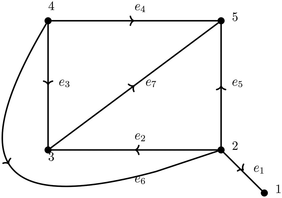
Network $\mathcal{G}$ $$Q(\mathcal{G})=\left[\begin{array}{ccccccc}-1& 0& 0& 0& 0& 0& 0\\ 1& 1& 0& 0& 1& -1& 0\\ 0& -1& -1& 0& 0& 0& 1\\ 0& 0& 1& 1& 0& 1& 0\\ 0& 0& 0& -1& -1& 0& -1\end{array}\right].$$

Now, partition the matrix Q as $\left[\begin{array}{c}{Q}_1\\ Q_2\end{array}\right]$, where $Q_1=\left[\begin{array}{ccccccc}-1& 0& 0& 0& 0& 0& 0\\ 1& 1& 0& 0& 1& -1& 0\\ 0& -1& -1& 0& 0& 0& 1\\ 0& 0& 1& 1& 0& 1& 0\end{array}\right]$ and $Q_2=\left[\begin{array}{ccccccc}0& 0& 0& -1& -1& 0& -1\end{array}\right]$. By substitution, we get $Q_1^T{(Q_1{Q}_1^T)}^{-1}=\frac{1}{4}\left[\begin{array}{cccc}-4& 0& 0& 0\\ 1& 1& -1& 0\\ 0& 0& -1& 1\\ 1& 1& 1& 2\\ 2& 2& 1& 1\\ -1& -1& 0& 1\\ 1& 1& 2& 1\end{array}\right]$ and using Eq. (3)(3) $$Q^{†}=\left[\begin{array}{cc}{Q}_1{}^T{(Q_1{Q}_1{}^T)}^{-1}& 0\end{array}\right](I-\frac{1}{n}J).$$(3) , we get the Moore-Penrose inverse of Q as (5) $$\begin{array}{c}{Q}^{†}=\left[\begin{array}{cc}{Q}_1^T{(Q_1{Q}_1^T)}^{-1}& 0\end{array}\right](I-\frac{1}{5}{J}_5)\\ \hspace{1em}=\frac{1}{5}\left[\begin{array}{ccccc}-4& 1& 1& 1& 1\\ 1& 1& -3/2& -1/4& -1/4\\ 0& 0& -5/4& 5/4& 0\\ 0& 0& 0& 5/4& -5/4\\ 1& 1& -1/4& -1/4& -3/2\\ -1& -1& 1/4& 3/2& 1/4\\ 0& 0& 5/4& 0& -5/4\end{array}\right]\mathrm{}.\end{array}$$(5)

3.3 Interpretation of Moore-Penrose inverse

The jth column of $Q^{†}$ represents the minimum flow through each of the edges required to achieve the net inflow of $\frac{4}{5}$ at jth vertex and $\frac{-1}{5}$ at remaining vertices. The flow quantities represented by first column is shown in the network. The minus sign indicates that the flow is in the direction opposite to the direction of the edge. In the following, we interpret the first column of Moore-Penrose inverse given in Eq. (5)(5) $$\begin{array}{c}{Q}^{†}=\left[\begin{array}{cc}{Q}_1^T{(Q_1{Q}_1^T)}^{-1}& 0\end{array}\right](I-\frac{1}{5}{J}_5)\\ \hspace{1em}=\frac{1}{5}\left[\begin{array}{ccccc}-4& 1& 1& 1& 1\\ 1& 1& -3/2& -1/4& -1/4\\ 0& 0& -5/4& 5/4& 0\\ 0& 0& 0& 5/4& -5/4\\ 1& 1& -1/4& -1/4& -3/2\\ -1& -1& 1/4& 3/2& 1/4\\ 0& 0& 5/4& 0& -5/4\end{array}\right]\mathrm{}.\end{array}$$(5) .

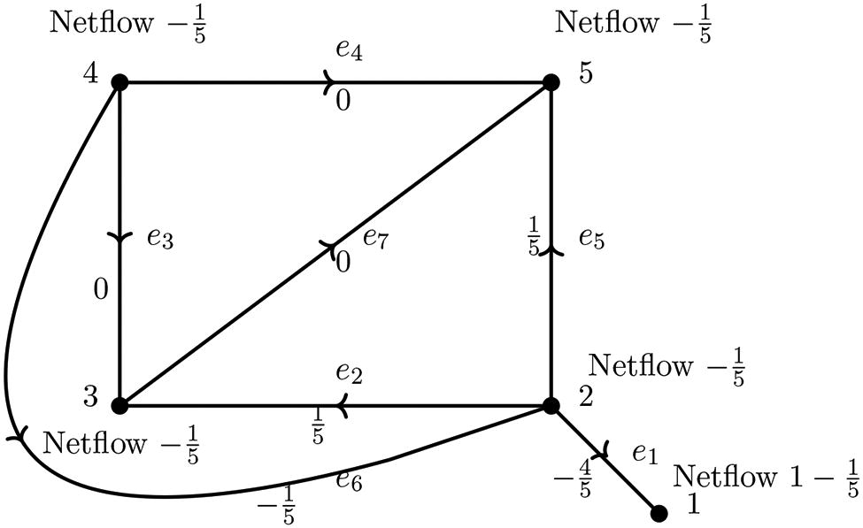
The first column of $Q^{†}$ represents the minimum flow required through each arc of $\mathcal{G}$ to achieve the net inflow of $\frac{4}{5}$ at node 1 and $\frac{-1}{5}$ at remaining nodes, which is nearest to the desired net inflow of 1 at node 1 and 0 elsewhere.

Example 3.3.

Consider the tree $\mathcal{T}$ given below.

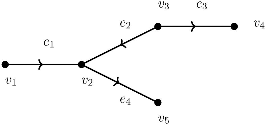
The incidence matrix of $\mathcal{T}$ is $$Q=\left[\begin{array}{cccc}1& 0& 0& 0\\ -1& -1& 0& 1\\ 0& 1& 1& 0\\ 0& 0& -1& 0\\ 0& 0& 0& -1\end{array}\right]$$

On partitioning Q as in (2), we get $Q_1=\left[\begin{array}{cccc}1& 0& 0& 0\\ -1& -1& 0& 1\\ 0& 1& 1& 0\\ 0& 0& -1& 0\end{array}\right]$, which is invertible. Now, using (4), the Moore-Penrose inverse of Q is given by (6) $$Q^{†}=\left[\begin{array}{cc}{Q}_1^{-1}& 0\end{array}\right](I-\frac{1}{5}{J}_5)=\frac{1}{5}\left[\begin{array}{ccccc}4& -1& -1& -1& -1\\ -2& -2& 3& 3& -2\\ 1& 1& 1& -4& 1\\ 1& 1& 1& 1& -4\end{array}\right].$$(6)

3.4 By bordering Q

Given any m × n matrix A of rank r, one may obtain a bordered matrix of size $(m+n-r)\times (m+n-r)$ in the form $T=\left[\begin{array}{cc}A& P\\ Q& 0\end{array}\right]$, where columns of P are the basis for $\mathcal{N}(A^T)$ and the rows of Q are the basis for $\mathcal{N}(A)$, to obtain the Moore-Penrose inverse in the block of $T^{-1}$ corresponding to A in T. Readers are referred to [13] and [7] for more details.

In the context of $\mathcal{G}$ being a tree, the corresponding incidence matrix is full column rank matrix with $\mathcal{N}(Q^T)$ is $\left\{\mathbf{1}\right\}$. Therefore, $T=\left[\begin{array}{cc}Q& \mathbf{1}\end{array}\right]$ is invertible and Moore-Penrose inverse of Q is given by $T^{-1}\left[\begin{array}{c}{I}_{n-1}\\ 0\end{array}\right]$.

Example 3.4.

For the tree $\mathcal{T}$ given in Example 3.3, we have $$T=\left[\begin{array}{c}Q|\mathbf{1}\end{array}\right]=\left[\begin{array}{ccccc}1& 0& 0& 0& 1\\ -1& -1& 0& 1& 1\\ 0& 1& 1& 0& 1\\ 0& 0& -1& 0& 1\\ 0& 0& 0& -1& 1\end{array}\right].$$and $$T^{-1}=\frac{1}{5}\left[\begin{array}{ccccc}4& -1& -1& -1& -1\\ -2& -2& 3& 3& -2\\ 1& 1& 1& -4& 1\\ 1& 1& 1& 1& -4\\ 1& 1& 1& 1& 1\end{array}\right].$$

Thus, the Moore-Penrose inverse of Q is given by $Q^{†}=T^{-1}\left[\begin{array}{c}{I}_4\\ 0\end{array}\right]=\frac{1}{5}\left[\begin{array}{ccccc}4& -1& -1& -1& -1\\ -2& -2& 3& 3& -2\\ 1& 1& 1& -4& 1\\ 1& 1& 1& 1& -4\end{array}\right]$.

4 Generalized inverses of weighted graphs

The Laplacian matrix and its generalized inverse have a greater significance in the study of networks. Klein and Randić in [12] introduced a new notion called the resistance distance in a graph, which is different from the conventional distance(called graphical distance) in a graph. The graphical distance between the vertices a and b in the graphs ${\mathcal{G}}_1,{\mathcal{G}}_2$ and ${\mathcal{G}}_3$ given below are all equal to 2. However, in the graph ${\mathcal{G}}_2$ or ${\mathcal{G}}_3$, the number of paths between a and b is more than one. In other words, a and b have better communication in these graphs. One might think of a real life example of traveling between the cities a and b. Fewer the number of routes connecting a and b, the more is the traffic, making it more difficult to travel from one city to another.

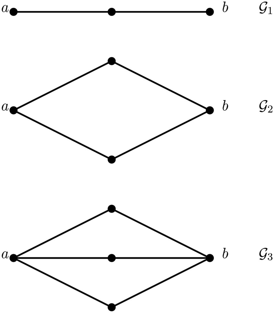
The ease of communication between a and b increases as we go from graph ${\mathcal{G}}_1$ to ${\mathcal{G}}_2$ to ${\mathcal{G}}_3$. However, the usual distance between a and b is the same for all the three graphs.

The resistance distance introduced in [12] is based on the electric network theory and it has the characteristic property of multiple-route distance diminishment. They considered each edge of a graph as a fixed resistor and defined the resistance distance between two vertices as the effective resistance between those two vertices.

Throughout this section, the graph $\mathcal{G}$ is simple, connected and edges (i, j) are associated with a strictly positive number (say w_ij). Adjacency matrix $A(\mathcal{G})$ (or simply A) is with entries equal to the reciprocal of the weight if the corresponding vertices are adjacent and equal to zero, otherwise. The degree of each vertex is the sum of reciprocal of the weights of the edges incident with it. The degree matrix Δ is a diagonal matrix in which the (i, i)th entry is the degree of ith vertex. The distance matrix D is defined such that the (i, j)th entry is the minimum of length of paths between v_i and v_j, where the length of path is the sum of weights of edges. The Laplacian matrix of the graph $\mathcal{G}$ is $\Delta -A$. It may be noted easily that $\mathcal{C}(L)={\left\{\mathbf{1}\right\}}^{\perp }$ and is of rank n – 1.

Using Kirchhoff’s law and Ohm’s law, it is proved in [12] that the resistance distance (effective resistance) between the ith vertex and jth vertex is given by (7) $$r_{ij}={(f_{ij})}^T{L}^{†}{f}_{ij}=l_{ii}^{+}+l_{jj}^{+}-2l_{ij}^{+},$$(7) where $f_{ij}=e_i-e_j$ and $l_{ij}^{+}$ is the (i, j)th entry of $L^{†}$. In fact, with $\nabla$ being the diagonal matrix whose diagonal entries are the diagonal entries of $L^{†}$, the matrix (8) $$R=\nabla J+J\nabla -2L^{†}$$(8) is called the resistance matrix.

Since it has been noted that L is a positive semidefinite matrix (see, [11]), the above “resistance distance” is a distance function on ${\left\{\mathbf{1}\right\}}^{\perp }$.

We list some interesting properties of generalized inverses of Laplacian matrix of a weighted graph $\mathcal{G}$.

Theorem 4.1.

Given a graph $\mathcal{G}$, the following hold.

• (ii)If $\mathcal{G}$ is a tree, for a column matrix τ whose ith entry is $2\text{-}\mathrm{deg}(v_i)$ (here $\mathrm{deg}$ refers to the degree of vertex in the unweighted graph $\mathcal{G}$) and the distance matrix D, we have (9) $$LD+2I=\tau {\mathbf{1}}^T.$$(9)

This in turn gives that $-\frac{1}{2}D$ is a generalized inverse of L and D = R.

• (ii) If $\mathcal{G}$ is any connected graph, then $-\frac{1}{2}R$ is generalized inverse of L.

Proof.

The Eq. (9)(9) $$LD+2I=\tau {\mathbf{1}}^T.$$(9) of part 1 of the above theorem could be verified easily by substitution, noting that distance between the adjacent vertices in a tree is same as the weight of edge incident with them. $-\frac{1}{2}D$ is a generalized inverse of L could be proved using Eq. (9)(9) $$LD+2I=\tau {\mathbf{1}}^T.$$(9) and the fact that ${\mathbf{1}}^{T}L=0$.

Since $f_{ij}\perp \mathbf{1}$ and $\mathcal{C}(L)={\left\{\mathbf{1}\right\}}^{\perp }$, we get $f_{ij}^T{L}^{-}{f}_{ij}$ is invariant under the choice of L^– and therefore $d_{ij}=f_{ij}^T(-\frac{1}{2}D)f_{ij}=f_{ij}^T{L}^{†}{f}_{ij}=r_{ij}$, proving that R = D.

For the proof of part (ii), we refer to Lemma 1 of [2]. □

Now, we will discuss different methods of constructing Moore-Penrose inverse of L.

4.1 Inverse complemented matrix method

In [10], in the more general context of ring elements, it has been proved that every reflexive generalized inverse of a square matrix could be obtained by using suitable inverse complement. The matrix version of the same result in the case of Moore-Penrose inverse is given below.

Theorem 4.2.

For any square matrix A of size n × n and any matrix C such that A + C is invertible and $A^{*}C=A{C}^{*}=0$, the Moore-Penrose inverse of A is given by (10) $$A^{†}={(A+C)}^{-1}A{(A+C)}^{-1}.$$(10)

Further, for any orthogonal projection P onto $\mathcal{C}(A^T)$ and orthogonal projection Q onto $\mathcal{C}(A)$, we get $A^{†}=P{(A+C)}^{-1}={(A+C)}^{-1}Q$.

Since $\mathbf{1}\perp \mathcal{C}(L)$ and L is symmetric, the following theorem follows as corollary to the Theorem 4.2.

Theorem 4.3.

If L is the Laplacian matrix of a weighted graph $\mathcal{G}$, we have (11) $$\begin{array}{c}{L}^{†}={(L+\lambda J)}^{-1}(I-\frac{1}{n}J)\\ =(I-\frac{1}{n}J){(L+\lambda J)}^{-1}={(L+\lambda J)}^{-1}-\frac{1}{\lambda n^2}J,\end{array}$$(11) for any nonzero λ.

By taking $\lambda =\frac{1}{n}$ in the expression Eq. (11)(11) $$\begin{array}{c}{L}^{†}={(L+\lambda J)}^{-1}(I-\frac{1}{n}J)\\ =(I-\frac{1}{n}J){(L+\lambda J)}^{-1}={(L+\lambda J)}^{-1}-\frac{1}{\lambda n^2}J,\end{array}$$(11) , we get $$L^{†}={(L+\frac{1}{n}J)}^{-1}-\frac{1}{n}J.$$

In the following example, we find the Moore-Penrose inverse of Laplacian matrix of a network using Theorem 4.3 and so obtained Moore-Penrose inverse is used to find the resistance matrix of the network.

Example 4.4.

Consider the electrical network $\mathcal{G}$ given below, for which the Laplacian matrix is given by $$L=\left[\begin{array}{cccc}7/2& -1/2& -1& -2\\ -1/2& 5/6& -1/3& 0\\ -1& -1/3& 17/6& -3/2\\ -2& 0& -3/2& 7/2\end{array}\right].$$

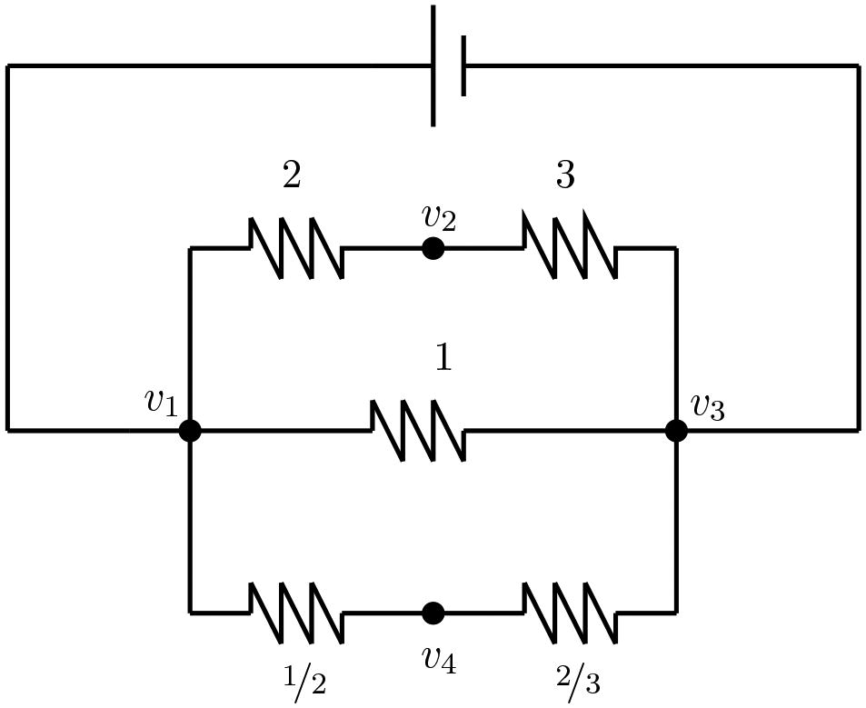
Network $\mathcal{G}$

Now, ${(L+J_4)}^{-1}=\frac{1}{144}\left[\begin{array}{cccc}37& -19& 5& 13\\ -19& 109& -23& -31\\ 5& -23& 43& 11\\ 13& -31& 11& 43\end{array}\right]$ and hence by taking λ = 1 in Eq. (11)(11) $$\begin{array}{c}{L}^{†}={(L+\lambda J)}^{-1}(I-\frac{1}{n}J)\\ =(I-\frac{1}{n}J){(L+\lambda J)}^{-1}={(L+\lambda J)}^{-1}-\frac{1}{\lambda n^2}J,\end{array}$$(11) , the Moore-Penrose inverse of L is given by $$L^{†}={(L+J_4)}^{-1}(I-\frac{1}{4}{J}_4)=\frac{1}{72}\left[\begin{array}{cccc}14& -14& -2& 2\\ -14& 50& -16& -20\\ -2& -16& 17& 1\\ 2& -20& 1& 17\end{array}\right].$$

Therefore, the resistance matrix is $$R=\nabla J+J\nabla -2L^{†}=\left[\begin{array}{cccc}0& 23/18& 35/72& 3/8\\ 23/18& 0& 11/8& 107/72\\ 35/72& 11/8& 0& 4/9\\ 3/8& 107/72& 4/9& 0\end{array}\right].$$

The (i, j)th entry of R represents the resistance distance between the vertices v_i and v_j. That is, the resistance distance between the vertices v₁ and v₂ is $r_{12}=\frac{23}{18}$ and the resistance distance between the vertices v₂ and v₄ is $r_{24}=\frac{107}{72}$ and so on.

4.2 Bordering method

For any m × n matrix of rank r, it has been proved in [13] that the bordered matrix $T=\left[\begin{array}{cc}A& P\\ Q& 0\end{array}\right]$, where P is $m\times (m-r)$ matrix with $\mathcal{C}(A)\perp \mathcal{C}(P)$ and Q is $n\times (n-r)$ matrix with $\mathcal{R}(A)\perp \mathcal{R}(Q)$, is invertible and the inverse is useful in obtaining the Moore-Penrose inverse of A. In fact, he showed that the block G₁₁ in the matrix $T^{-1}=\left[\begin{array}{cc}{G}_{11}& G_{12}\\ G_{21}& G_{22}\end{array}\right]$, correspond to A in T, is the Moore-Penrose inverse of A, G₁₂ is a least squares g-inverse (moreover, a right inverse) of Q, and G₂₁ is a minimum norm g-inverse (moreover, a left inverse) of P.

Since $\mathcal{C}(L)={\left\{\mathbf{1}\right\}}^{\perp }$ and $\mathcal{R}(L)={\left\{\mathbf{1}\right\}}^{\perp }$, it follows that the matrix $T=\left[\begin{array}{cc}L& \mathbf{1}\\ {\mathbf{1}}^T& 0\end{array}\right]$ is invertible and the Moore-Penrose inverse is given by (12) $$L^{†}=\left[\begin{array}{cc}{I}_n& 0\end{array}\right]T^{-1}\left[\begin{array}{c}{I}_n\\ 0\end{array}\right].$$(12)

Example 4.5.

Consider the Laplacian matrix L of the network given in Example 4.4, for which $$T=\left[\begin{array}{cc}L& \mathbf{1}\\ {\mathbf{1}}^T& 0\end{array}\right]=\left[\begin{array}{ccccc}7/2& -1/2& -1& -2& 1\\ -1/2& 5/6& -1/3& 0& 1\\ -1& -1/3& 17/6& -3/2& 1\\ -2& 0& -3/2& 7/2& 1\\ 1& 1& 1& 1& 0\end{array}\right]$$and $$T^{-1}=\frac{1}{72}\left[\begin{array}{ccccc}14& -14& -2& 2& 18\\ -14& 50& -16& -20& 18\\ -2& -16& 17& 1& 18\\ 2& -20& 1& 17& 18\\ 18& 18& 18& 18& 0\end{array}\right].$$

Thus, the Moore-Penrose inverse of L is given by $$\left[\begin{array}{cc}{I}_4& 0\end{array}\right]T^{-1}\left[\begin{array}{c}{I}_4\\ 0\end{array}\right]=\frac{1}{72}\left[\begin{array}{cccc}14& -14& -2& 2\\ -14& 50& -16& -20\\ -2& -16& 17& 1\\ 2& -20& 1& 17\end{array}\right].$$

4.3 Partition method

Let the Laplacian matrix of a graph be partitioned as (13) $$L=\left[\begin{array}{cc}{L}_{11}& L_{12}\\ L_{21}& L_{22}\end{array}\right],$$(13) where L₁₁ is the $n-1\times n-1$ principal submatrix of L. Since $\text{rank}(L)=n-1$ and $L\mathbf{1}={\mathbf{1}}^{T}L=0$, the submatrix L₁₁ is a full rank matrix. Noting that $I-\frac{1}{n}J$ is a projection onto $\mathcal{C}(L)=\mathcal{R}(L)$ and that $\left[\begin{array}{cc}{L}_{11}^{-1}& 0\\ 0& 0\end{array}\right]$ is a generalized inverse of L, and therefore the Moore-Penrose inverse of L is given by (14) $$L^{†}=(I-\frac{1}{n}J)\left[\begin{array}{cc}{L}_{11}^{-1}& 0\\ 0& 0\end{array}\right](I-\frac{1}{n}J).$$(14)

Example 4.6.

Partitioning the Laplacian matrix L of network considered in Example 4.4 as in Eq. (13)(13) $$L=\left[\begin{array}{cc}{L}_{11}& L_{12}\\ L_{21}& L_{22}\end{array}\right],$$(13) , we get $L_{11}=\left[\begin{array}{ccc}7/2& -1/2& -1\\ -1/2& 5/6& -1/3\\ -1& -1/3& 17/6\end{array}\right],L_{12}=\left[\begin{array}{c}-2\\ 0\\ -3/2\end{array}\right],L_{21}=L_{12}^T$ and $L_{22}=\frac{7}{2}$. Now, using Eq. (14)(14) $$L^{†}=(I-\frac{1}{n}J)\left[\begin{array}{cc}{L}_{11}^{-1}& 0\\ 0& 0\end{array}\right](I-\frac{1}{n}J).$$(14) , the Moore-Penrose inverse of L is given by $$\begin{array}{c}{L}^{†}=(I-\frac{1}{4}{J}_4)\left[\begin{array}{cc}{L}_{11}^{-1}& 0\\ 0& 0\end{array}\right](I-\frac{1}{4}{J}_4)\\ =\frac{1}{72}\left[\begin{array}{cccc}14& -14& -2& 2\\ -14& 50& -16& -20\\ -2& -16& 17& 1\\ 2& -20& 1& 17\end{array}\right].\end{array}$$

As a consequence of Eq. (14)(14) $$L^{†}=(I-\frac{1}{n}J)\left[\begin{array}{cc}{L}_{11}^{-1}& 0\\ 0& 0\end{array}\right](I-\frac{1}{n}J).$$(14) , the resistance distance between a fixed vertex (say v_n) and the rest are given as in the following theorem.

Theorem 4.7.

If we partition the Laplacian matrix L in the following form $$L=\left[\begin{array}{cc}{L}_{11}& L_{12}\\ L_{21}& L_{22}\end{array}\right],$$where L₁₁ is the first principal submatrix of order n – 1 of L. Then the resistance distance between the vertices $v_1,\dots ,v_{n-1}$ and v_n is given by the corresponding diagonal entries of $L_{11}^{-1}$. In other words, $$r_{in}={(L_{11}^{-1})}_{ii}=\lambda {(\text{adj}(L_{11}))}_{ii},$$ where λ is the reciprocal of number of spanning trees in the graph.

Proof.

Since f_ij is in $\mathcal{C}(L)=\mathcal{R}(L),f_{ij}^T{L}^{-}{f}_{ij}$ is invariant under the choices of L^– . Now the theorem follows immediately from the definition of resistance distance and the fact $\left[\begin{array}{cc}{L}_{11}^{-1}& 0\\ 0& 0\end{array}\right]$ is a generalized inverse of L. □

4.4 Moore-Penrose inverse of some special graphs

Given a complete graph ${\mathcal{K}}_p$ and a complete bipartite graph ${\mathcal{K}}_{p,q}$ (both are unweighted), the corresponding Laplacian matrices are of the form $pI-J_p$ and $\left[\begin{array}{cc}p{I}_q& -J_{pq}\\ -J_{qp}& q{I}_p\end{array}\right]$, respectively. Further, it may be noted by direct verification that (15) $${(p{I}_q+J_q)}^{-1}=\frac{1}{p}(I_q-\frac{1}{p+q}{J}_q).$$(15)

Above information is useful in proving the following theorem.

Theorem 4.8.

For complete graph ${\mathcal{K}}_p$ and complete bipartite graph ${\mathcal{K}}_{p,q}$, both are unweighted, we have

1. ${(L({\mathcal{K}}_p))}^{†}=\frac{1}{p}(I_p-\frac{1}{p}{J}_p)=\frac{1}{p^2}L$ (16)

2. ${(L({\mathcal{K}}_{p,q}))}^{†}=\frac{1}{pq}\left[\begin{array}{cc}p{I}_p& 0\\ 0& q{I}_q\end{array}\right]-\frac{1}{{(p+q)}^2}\left[\begin{array}{cc}\lambda J_p& J_{pq}\\ J_{qp}& \mu J_q\end{array}\right],$ (17)

where $\lambda =\frac{1}{q}(p+2q)$ and $\mu =\frac{1}{p}(q+2p)$.

Proof.

(i) The Laplacian matrix of ${\mathcal{K}}_p$ has all of its diagonal entries equal to p – 1 and off diagonal entries equal to –1 i.e., $L=p{I}_p-J_p$ and hence $L+J_p=p{I}_p$. Now, by taking λ = 1 in Eq 11(11) $$\begin{array}{c}{L}^{†}={(L+\lambda J)}^{-1}(I-\frac{1}{n}J)\\ =(I-\frac{1}{n}J){(L+\lambda J)}^{-1}={(L+\lambda J)}^{-1}-\frac{1}{\lambda n^2}J,\end{array}$$(11) , we get $${(L({\mathcal{K}}_p))}^{†}=\frac{1}{p}{I}_p-\frac{1}{p^2}{J}_p=\frac{1}{p^2}(p{I}_p-J_p)=\frac{1}{p^2}L.$$

(ii) Note that the Laplacian of ${\mathcal{K}}_{p,q}$ is $$L({\mathcal{K}}_{p,q})=\left[\begin{array}{cc}q{I}_p& -J_{pq}\\ -J_{qp}& p{I}_q\end{array}\right],$$and hence, (18) $$L+J=\left[\begin{array}{cc}q{I}_p+J_p& 0\\ 0& p{I}_q+J_q\end{array}\right].$$(18)

Now, by taking λ = 1 in Eq. (11)(11) $$\begin{array}{c}{L}^{†}={(L+\lambda J)}^{-1}(I-\frac{1}{n}J)\\ =(I-\frac{1}{n}J){(L+\lambda J)}^{-1}={(L+\lambda J)}^{-1}-\frac{1}{\lambda n^2}J,\end{array}$$(11) and using Eq. (15)(15) $${(p{I}_q+J_q)}^{-1}=\frac{1}{p}(I_q-\frac{1}{p+q}{J}_q).$$(15) , we obtain the Moore-Penrose inverse as in Eq. (17). □

Theorem 4.9.

Let K_p and $K_{p,q}$ denote the complete graph and complete bipartite graphs, both are unweighted, respectively.

(i) The resistance distance between any two distinct vertices of ${\mathcal{K}}_p$ is $\frac{2}{p}$ and the resistance matrix is $$R(K_p)=\frac{2}{p}(J_p-I_p).$$

(ii) Suppose v_i and v_j are two distinct vertices of ${\mathcal{K}}_{p,q}$ with bipartition (V ₁, V ₂). Then the resistance distance between v_i and v_j is given by $$r_{ij}=\{\begin{array}{cc}\frac{2}{q}\hfill & \text{ if }{v}_i\text{ and }{v}_j\text{ are in the same partition }{V}_1\hfill \\ \frac{2}{p}\hfill & \text{if }{v}_i\text{ and }{v}_j\text{ are in the same partition }{V}_2\hfill \\ \frac{p+q-1}{pq}\hfill & \text{ if }{v}_i\text{ and }{v}_j\text{ are in the different partitions}\hfill \end{array}$$and resistance matrix is given by $$R(K_{p,q})=\left[\begin{array}{cc}\frac{2}{q}{J}_p& \frac{p+q-1}{pq}{J}_{pq}\\ \frac{p+q-1}{pq}{J}_{qp}& \frac{2}{p}{J}_q\end{array}\right].$$

Proof.

The proof is immediate from the Eqs. (16), (17) and the definition of resistance distance. □

5 Conclusion

In this article, we have reviewed interesting applications of generalized inverses in the area of graph theory. Some of the existing results are rewritten focusing on the role of generalized inverses. Significance of Moore-Penrose inverse of incidence matrix of a directed graph in network flow analysis is studied. New methods of computing the Moore-Penrose inverse of incidence matrix and that of Laplacian matrix are provided.

References

- Bapat, R. B. (1997). Moore-penrose inverse of the incidence matrix of a tree. Linear Multilinear Algebra. 42: 159–167.
- Bapat, R. B. (2004). Resistance matrix of a weighted graph. MATCH Commun. Math. Comput. Chem. 50: 73–82.
- Bapat, R. B. (2014). Graphs and Matrices, 2nd ed. London: Springer-Verlag.
- Ben-Israel, A., Greville, T. N. E. (1974). Generalized Inverses: Theory and Applications, 2nd ed. New York: Springer.
- Bhat, K. N., Karantha, M. P., Eagambaram, N. (2021). Inverse complements of a matrix and its applications. J. Algebra Appl. 20(8): 1–12.
- Bollobás, B. (1998). Modern Graph Theory, 1st ed. New York: Springer-Verlag.
- Eagambaram, N. (1991). (i,j,…,k)-inverses via bordered matrices. Sankhya¯ Ser. A (1961–2002) 53(3): 298–308.
- Harary, F. (1969). Graph Theory, 1st ed. Boston, MA: Addison-Wesley.
- Ijiri, Y. (1965). On the generalized inverse of an incidence matrix. J. Soc. Indust. Appl. Math. 13(3): 827–836.
- Kelathaya, U., Varkady, S., Karantha, M. P. (2022). Inverse complements and strongly unit regular elements. J. Algebra Appl. 21(10): 1–11.
- Kirkland, S. J., Neumann, M., Shader, B. L. (1997). Distances in weighted trees and group inverse of Laplacian matrices. SIAM J. Matrix Anal. Appl. 18(4): 827–841.
- Klein, D. J., and Randić, M. (1993). Resistance distance. J. Math. Chem. 12: 81–95.
- Nomakuchi, K. (1980). On the characterization of generalized inverses by bordered matrices. Linear Algebra Appl. 33: 1–8.
- Prasad, K. M. (2012). An introduction to generalized inverse. In: Bapat, R. B., Kirkland, S., Prasad, K. M., Puntanen, S., eds. Lectures on Matrix and Graph Methods. Manipal, India: Manipal University Press, pp. 43–60.
- Prasad, K. M., Bhaskara Rao, K. P. S. (1996). On bordering of regular matrices. Linear Algebra Appl. 234: 245–259.
- Rao, C. R., Mitra, S. K. (1971). Generalized Inverses of Matrices and its Applications. New York: Wiley.