Stress of a graph and its computation

Abstract

Stress is a centrality measure determined by the shortest paths passing through the given vertex. Noting that adjacency matrix playing an important role in finding the distance and the number of shortest paths between given pair of vertices, an interesting expression and also an algorithm are presented to find stress using adjacency matrix. The results and algorithm are suitably adopted to obtain betweenness centrality measure. Further results are extended to the cases of Cartesian product $G\square H$ of graphs, corona graph $G°H$ and their special cases.

KEYWORDS:

• Centrality measure
• stress
• betweenness
• adjacency matrix
• distance matrix

AMS CLASSIFICATION:

• 05C12
• 05C50

1 Introduction

Centrality measures are among essential tools in network analysis. Depending on the given context, one can quantify the importance of a node or an edge in a network and hence one can identify crucial vertices or edges. In general, one can define centrality measure as a function f which assigns a real value $f(v)$ to every vertex v of a graph G. Many important centrality measures such as degree centrality, betweenness centrality, closeness centrality, eigenvector centrality are studied and used in the analysis of various networks. Readers are referred to [1, 6, 7, 12] for the details.

Stress is an important centrality measure introduced by Alfonso Shimbel; see [13]. Stress of a vertex in a graph is the number of shortest paths passing through that vertex. In spite of its significance in the applications (like in understanding responsible protein causing cancer in the protein-signaling network), studying its mathematical properties is not given a considerable attention. The articles [2, 8, 9] are few among the articles in recent days in which the properties of stress have been studied in the context of different graphs. Rather than counting the number of shortest paths passing through the vertex to find the stress, as done in these references, we consider the adjacency matrix to be an effective tool to compute the stress and present the algorithm for the same. Further, using the adjacency matrices of the graphs G and H, we compute the stress of the vertices in the Cartesian product $G\square H$ and the corona graph $G°H$. In Section 4, we provide algorithms to find the stress of vertices in the graphs using the results discussed in the Section 3.

2 Preliminaries

Throughout this paper, the graphs considered are simple, finite, undirected and connected graphs. The length of a shortest $u-v$ path is called the distance between the vertices u and v, and the same is denoted by $d_G(u,v)$ or simply $d(u,v)$, if the graph under discussion is clear. In a $u-v$ path given by $P(u,v)=(u=v_{i_1},v_{i_2},\dots ,v_{i_n}=v)$, the vertex $u=v_{i_1}$ is called origin and the vertex $v=v_{i_n}$ is terminus, and the vertices $v_{i_k},2\le k\le n-1$ are called the internal vertices of the path P. The set of shortest paths between the vertices u and v is denoted by $\mathcal{P}(u,v)$ and the set of shortest paths between u and v having w as an interior vertex is denoted by ${\mathcal{P}}_w(u,v)$. Further, we denote $\#\mathcal{P}(u,v)$ by $\eta (u,v)$ and $\#{\mathcal{P}}_w(u,v)$ by ${\eta }_w(u,v)$.

Definition 2.1 (Stress of a vertex, Stress of a graph)

Let G be a graph with $V(G)=\{v_1,v_2,\dots ,v_n\}$. The stress of a vertex v, denoted by $s{t}_G(v)$, is the number of shortest paths in G having v as an internal vertex. The stress of a graph G, denoted by $st(G)$, is given by ${\sum }_{i=1}^{n}st(v_i)$.

Every vertex sends information to every other vertex through shortest paths and stress is a centrality measure which measures the ability of a vertex in holding together the communicating vertices. Higher the number of shortest paths passing through a vertex, higher will be its stress. After Alfonso Shimbel introduced this notion of stress, not much theoretical investigation was done in this particular area. But, the articles [10, 11, 12] are a few evidences in which stress is used in the analysis of some biological networks. In the recent developments (see, [2, 8, 9]) some important properties of stress are explored. The expressions for the stress of vertices from some standard graphs such as paths, trees, cycles, wheels, complete bipartite etc., are discussed. Among the trees of order n, path graph is seen with maximum stress and star graph with minimum stress. It is found that stress of a block graph is the sum of the stress at the cut vertices. A graph is k-stress regular if stress of each of its vertices is k. Characterization of k-stress regular graphs can also be seen in the literature.

In the current paper we make use of the adjacency matrix of the graph to compute the stress of a vertex. For a graph G with n vertices $v_1,v_2,\dots ,v_n$, the adjacency matrix $A(G)=(a_{ij})$ is an $n\times n$ matrix, in which $a_{ij}=1$ if $v_i$ is adjacent with $v_j$ and $a_{ij}=0$ otherwise. For the same graph, the distance matrix $D(G)=(d_{ij})$ is the $n\times n$ matrix where $d_{ij}=d(v_i,v_j)$. Whenever the graph under discussion is clear from the context, we write A and D instead of $A(G)$ and $D(G)$, respectively, to denote the adjacency and distance matrices. Now, we introduce a notion of shortest path matrix $N(G)$ of graph G as in thefollowing.

Definition 2.2 (Shortest path matrix)

Given a connected graph G, the shortest path matrix of G denoted by $N(G)$ is an $n\times n$ matrix in which the iith entry ${\eta }_{ii}^G$ is 1 and ijth entry ${\eta }_{ij}^G$ represents the number of shortest paths between $v_i$ and $v_j$ ($i\ne j$), i.e., $\eta (v_i,v_j)$.

The notations $N(G)$ and ${\eta }_{ij}^G$ used in the above definition are replaced by N and ${\eta }_{ij}$, respectively, when the graph under discussion is clear from the context. It may be noted that for $i\ne j$, we have ${\eta }_{ij}=\#\mathcal{P}(v_i,v_j)$. Further, writing ${\eta }_{ii}=1$ in the above definition is for our computational convenience (representing the number of paths/walks of length zero from a vertex to itself!).

Other centrality measure which is computationally closer to stress is betweenness centrality measure.

Definition 2.3 (Betweenness Centrality)

Betweenness centrality measure of a vertex $v_k$, denoted by $C_B(v_k)$, is given by (1) $$C_B(v_k)=\sum _{\underset{i<j}{i,j\ne k}}\frac{{\eta }_{v_k}(v_i,v_j)}{\eta (v_i,v_j)}.$$(1)

In Section 3, we give an expression for computing betweenness centrality using the properties of adjacency matrix. Then using the same result, in the Section 4, we present an algorithm to compute this measure.

3 Computation of stress using adjacency matrix

Note that by joining any two paths having one common terminus vertex need not result in a shortest path. In fact, a $u-v-w$ path is a shortest path between u and w if and only if $d(u,v)+d(v,w)=d(u,w)$. The following lemma relates the stress of any vertex of graph G with the entries of $N(G)$.

Lemma 3.1.

If G is a connected graph with $N(G)=({\eta }_{ij})$, then for any vertex $v_k\in V(G)=\{v_1,v_2,\dots ,v_n\},$ (2) $$s{t}_G(v_k)=\sum _{\underset{d(v_i,v_k)+d(v_k,v_j)=d(v_i,v_j)}{\underset{i<j,i,j\ne k}{1\le i,j\le n}}}{\eta }_{ik}{\eta }_{kj}.$$(2)

Proof.

For any two vertices $v_i,v_j,i\ne j$, it may be noted that a shortest $v_i-v_j$ path will pass through a vertex $v_k$ if and only if (3) $$d(v_i,v_k)+d(v_k,v_j)=d(v_i,v_j).$$(3)

In the above case, any shortest $v_i-v_j$ path passing through $v_k$ is obtained by joining a shortest $v_i-v_k$ path with a shortest $v_k-v_j$ path, and vice versa. In other words, we have one-one correspondence between shortest paths $v_i-v_j$-paths passing through $v_k$ and pairs of shortest $v_i-v_k$ and $v_k-v_j$ paths. Therefore, if ${\eta }_{ik}$ and ${\eta }_{kj}$ denotes the number of shortest $v_i-v_k$ paths and $v_k-v_j$ paths, respectively, then the number of shortest paths between $v_i$ and $v_j$ passing through $v_k$ is given by the product ${\eta }_{ik}{\eta }_{kj}$. In other words, we have (4) $$\#{\mathcal{P}}_{v_k}(v_i,v_j)=\#\mathcal{P}(v_i,v_k)\times \#\mathcal{P}(v_k,v_j),$$(4) or simply, ${\eta }_{v_k}(v_i,v_j)=\eta (v_i,v_k)\eta (v_k,v_j)$. Now by referring to the Definition 2.1, the stress of $v_k$ is given by the sum of the products ${\eta }_{ik}{\eta }_{kj}$, where the summation is taken over all pair of vertices $v_i,v_j,i<j$ satisfying Eq. (3)(3) $$d(v_i,v_k)+d(v_k,v_j)=d(v_i,v_j).$$(3) , proving Eq. (2)(2) $$s{t}_G(v_k)=\sum _{\underset{d(v_i,v_k)+d(v_k,v_j)=d(v_i,v_j)}{\underset{i<j,i,j\ne k}{1\le i,j\le n}}}{\eta }_{ik}{\eta }_{kj}.$$(2) . Hence the lemma. ▪

It is well known that the entries of $A^p$ provide the number of walks of length p between the distinct vertices and the readers are referred to any standard text books like [4]. The following theorem follows immediately.

Theorem 3.2.

If G is a connected graph, then $d_{ij}$, the distance between $v_i$ and $v_j$ for $i\ne j$ is the least integer p for which the $i{j}^{\text{th}}$ entry of $A^p$ is nonzero. In such a case, ${\eta }_{ij}={(A^p)}_{ij}$.

In view of the above theorem the shortest path matrix $N(G)$ could be redefined as the matrix $N=({\eta }_{ij})$ such that ${\eta }_{ij}=\{\begin{array}{cc}\mathit{lcl}1,& \text{ for }i=j\\ {(A^p)}_{ij},& \text{ otherwise}\end{array}$, where p is the least integer for which the $i{j}^{\text{th}}$ entry of $A^p$ is nonzero. Now the following corollary is immediate.

Corollary 3.3.

If G is a graph with the adjacency matrix A, then for any vertex $v_k\in V(G)=\{v_1,v_2,\dots ,v_n\},$ (5) $$s{t}_G(v_k)=\sum _{\underset{d(v_i,v_k)+d(v_k,v_j)=d(v_i,v_j)}{\underset{i<j,i,j\ne k}{i,j=1}}}^n{\eta }_{ik}{\eta }_{kj},$$(5) where ${\eta }_{ij}=\{\begin{array}{cc}\mathit{lcl}1,& \text{ for }i=j\\ {(A^p)}_{ij},& \text{ otherwise}\end{array}$ and p is the least integer for which the ijth entry of $A^p$ is nonzero.

In the following theorem, we present an expression to compute betweeness centrality of a vertex in G using the shortest path matrix $N(G)$ of G. The proof is immediate from the definition of betweenness centrality and the Eq. (4)(4) $$\#{\mathcal{P}}_{v_k}(v_i,v_j)=\#\mathcal{P}(v_i,v_k)\times \#\mathcal{P}(v_k,v_j),$$(4) .

Theorem 3.4.

If G is a graph with the adjacency matrix A, then for any vertex $v_k\in V(G)=\{v_1,v_2,\dots ,v_n\},$ the betweenness centrality of $v_k$ is given by (6) $$C_B(v_k)=\sum _{\underset{d(v_i,v_k)+d(v_k,v_j)=d(v_i,v_j)}{\underset{i<j,i,j\ne k}{i,j=1}}}^n\frac{{\eta }_{ik}{\eta }_{kj}}{{\eta }_{ij}},$$(6) where ${\eta }_{ij}=\{\begin{array}{cc}\mathit{lcl}1,& \text{ for }i=j\\ {(A^p)}_{ij},& \text{ otherwise,}\end{array}$ and p is the least integer for which the ijth entry of $A^p$ is nonzero.

We next discuss on how the adjacency matrices of the graphs G and H are useful in determining the stress of verticesin $G\square H$.

3.1 Stress of vertices in the Cartesian product

Definition 3.5 (Cartesian product of graphs).

The Cartesian product of two graphs G and H, denoted by $G\square H$, is a graph with vertex set $V(G)\times V(H)$, where two vertices $(u_1,v_1)$ and $(u_2,v_2)$ are adjacent if $u_1=u_2$ and $v_1{v}_2\in E(H)$ or $v_1=v_2$ and $u_1{u}_2\in E(G).$

It may be noted that in the case of Cartesian product $G\square H$, the corresponding adjacency matrix, distance matrix and shortest path matrix are written by considering the pairs of vertices in the lexicographical ordering as column and row indices. The number of shortest paths between any two vertices $(u_{i_1},v_{j_1})$ and $(u_{i_2},v_{j_2})$ in the Cartesian product $G\square H$ is studied in literature [3, 5] and given by (7) $${\eta }_{(u_{i_1},v_{j_1}),(u_{i_2},v_{j_2})}^{G\square H}=\left(\begin{array}{c}{d}_G(u_{i_1},u_{i_2})+d_H(v_{j_1},v_{j_2})\\ d_G(u_{i_1},u_{i_2})\end{array}\right){\eta }_{i_1{i}_2}^G{\eta }_{j_1{j}_2}^H.$$(7)

For the convenience of the reader, we provide a detailed but independent explanation on computing the number of shortest paths between the vertices of Cartesian product of twographs.

To start with, consider a tridiagonal $n\times n$ matrix of the form $$X=\left[\begin{array}{cccccc}x& 1& 0& 0& \dots & 0\\ 1& x& 1& 0& \dots & 0\\ 0& 1& x& 1& \dots & 0\\ ⋮& ⋮& ⋮& \ddots & ⋮& \\ 0& 0& 0& \dots & \dots & x\end{array}\right]$$and the matrices $X^t,t=1,2,\dots$ to observe the following:

1. ${(X^t)}_{1n}=0$ for all $t<n-1$ and ${(X^{n-1})}_{1n}=1$

2. The highest power of x in $1j\text{th}$ term of $X^k$ is $x^{k-j+1}$ with the coefficient (8) $$s_k(j)=\{\begin{array}{cc}1\hfill & \text{for}j=1\hfill \\ s_{k-1}(j-1)+s_{k-1}(j)\hfill & \text{for}1\ne j\le k+1.\hfill \end{array}$$(8)

3. By taking $s_0(1)=1$ and $s_k(0)=s_k(j)=0$ for $j>k+1$, we observe that $s_k(j)$ generates the Pascal’s triangle $$\begin{array}{cc}{s}_0\hfill & =1,0,0,0,0,0,\dots \hfill \\ s_1=1,1,0,0,0,0,\dots \hfill & \hfill \\ s_2\hfill & =1,2,1,0,0,0,\dots \hfill \\ s_3=1,3,3,1,0,0,\dots \hfill & \hfill \\ s_4\hfill & =1,4,6,4,1,0,\dots \hfill \\ ⋮\hfill & \hfill \end{array}$$

and in fact, (9) $$s_k(j)=\left(\begin{array}{c}k\\ j-1\end{array}\right)\hspace{1em}\text{for }1\le j\le k+1,$$(9)

the coefficient of $x^j$ in the binomial expansion of ${(x+1)}^k$.

1. Now by considering path graphs $P_m:(v_1,\dots ,v_m)$ and $P_n:(w_1,\dots ,w_n)$ of length $m-1$ and $n-1$, we observe that the adjacency matrix of the Cartesian product $P_m\square P_n$ is the block matrix of size $m\times m$ given by (10) $$A=\left[\begin{array}{cccccc}B& I& 0& 0& \dots & 0\\ I& B& I& 0& \dots & 0\\ 0& I& B& I& \dots & 0\\ ⋮& ⋮& ⋮& \ddots & ⋮& \\ 0& 0& 0& \dots & \dots & B\end{array}\right],$$(10)

where B is the adjacency matrix of $P_n$ of size $n\times n$ and of the form (11) $$\left[\begin{array}{ccccccc}0& 1& 0& 0& \dots & 0& 0\\ 1& 0& 1& 0& \dots & 0& 0\\ 0& 1& 0& 1& \dots & 0& 0\\ ⋮& ⋮& ⋮& \ddots & ⋮& & \\ 0& 0& 0& \dots & \dots & 1& 0\end{array}\right].$$(11)

Since the vertices of $P_m\square P_n$ are arranged in the lexicographical ordering, referring to Theorem 3.2, the distance between $(v_1,w_1)$ and $(v_m,w_n)$ is given by the least positive integer k for which $(1,mn)$th entry of $A^k$ is nonzero. This is possible when $B^{n-1}$ appears in $(1,m)\text{th}$ block of $A^k$. From the observations (i)–(iii), we get that k must be $m+n-2$ and $(1,mn)$th entry of $A^{m+n-2}$ is the coefficient of $B^{n-1}$ in the $(1,m)\text{th}$ block and given by (12) $$s_{m+n-2}(m)=\left(\begin{array}{c}m+n-2\\ m-1\end{array}\right)$$(12)

1. If $l_1$ is the length of a path graph $P_1(u_1,u_2)$ and $l_2$ is the length of a path graph $P_2(v_1,v_2)$, then referring to Eq. (12)(12) $$s_{m+n-2}(m)=\left(\begin{array}{c}m+n-2\\ m-1\end{array}\right)$$(12) we have $(\begin{array}{c}{l}_1+l_2\\ l_1\end{array})(=(\begin{array}{c}{d}_{P_1}(u_1,u_2)+d_{P_2}(v_1,v_2)\\ d_{P_1}(u_1,u_2)\end{array}))$ number of paths between $(u_1,v_1)$ and $(u_2,v_2)$ in the $P_1\square P_2$.

2. Noting that each pair of shortest paths in the factor graphs produce as many number of shortest paths as mentioned in Eq. (12)(12) $$s_{m+n-2}(m)=\left(\begin{array}{c}m+n-2\\ m-1\end{array}\right)$$(12) in the Cartesian product, the total number of shortest paths between any two vertices in the Cartesian product is as given in Eq. (7)(7) $${\eta }_{(u_{i_1},v_{j_1}),(u_{i_2},v_{j_2})}^{G\square H}=\left(\begin{array}{c}{d}_G(u_{i_1},u_{i_2})+d_H(v_{j_1},v_{j_2})\\ d_G(u_{i_1},u_{i_2})\end{array}\right){\eta }_{i_1{i}_2}^G{\eta }_{j_1{j}_2}^H.$$(7) .

In the following theorem, we will present an expression to find the stress of a vertex in the Cartesian product $G\square H$ with reference to the details from the factor graphs.

Theorem 3.6.

For any connected graphs G and H, the stress of a vertex $(u_i,v_j)$ in $G\square H$ is given by (13) $$\begin{array}{cc}s{t}_{G\square H}(u_i,v_j)=\frac{1}{2}\sum \left[\left(\begin{array}{c}{d}_G(u_i,u_{i_1})+d_H(v_j,v_{j_1})\\ d_G(u_i,u_{i_1})\end{array}\right){\eta }_{i{i}_1}^G{\eta }_{j{j}_1}^H\right]\hfill & \hfill \\ \hspace{1em}\times \left[\left(\begin{array}{c}{d}_G(u_i,u_{i_2})+d_H(v_j,v_{j_2})\\ d_G(u_i,u_{i_2})\end{array}\right){\eta }_{i{i}_2}^G{\eta }_{j{j}_2}^H\right],\hfill & \hfill \end{array}$$(13)

where the summation is taken over all the pairs of vertices $(u_{i_1},v_{j_1})$ and $(u_{i_2},v_{j_2})$ different from $(u_i,v_j)$ in $G\square H$ satisfying $d_G(u_{i_1},u_i)+d_G(u_i,u_{i_2})=d_G(u_{i_1},u_{i_2})$ and $d_H(v_{j_1},v_j)+d_H(v_j,v_{j_2})=d_H(v_{j_1},v_{j_2}).$

Proof.

Referring to Eq. (3)(3) $$d(v_i,v_k)+d(v_k,v_j)=d(v_i,v_j).$$(3) , note that any vertex $(u_i,v_j)$ denoted by x is an internal vertex in the shortest paths between the vertices $y=(u_{i_1},v_{j_2})$ and $z=(u_{i_2},v_{j_2})$ if and only if (14) $$d_{G\square H}(y,x)+d_{G\square H}(x,z)=d_{G\square H}(y,z),$$(14) equivalently, (15) $$\begin{array}{cc}{d}_G(u_{i_1},u_i)+d_G(u_i,u_{i_2})\hfill & =d_G(u_{i_1},u_{i_2})\hspace{1em}\text{and}\hfill \end{array}$$(15) $$d_H(v_{j_1},v_j)+d_H(v_j,v_{j_2})=d_H(v_{j_1},v_{j_2}).$$

Now referring to Eq. (4)(4) $$\#{\mathcal{P}}_{v_k}(v_i,v_j)=\#\mathcal{P}(v_i,v_k)\times \#\mathcal{P}(v_k,v_j),$$(4) in the Lemma 3.1, when the Eqs. (14)(14) $$d_{G\square H}(y,x)+d_{G\square H}(x,z)=d_{G\square H}(y,z),$$(14) and (15)(15) $$\begin{array}{cc}{d}_G(u_{i_1},u_i)+d_G(u_i,u_{i_2})\hfill & =d_G(u_{i_1},u_{i_2})\hspace{1em}\text{and}\hfill \end{array}$$(15) are satisfied, it follows that the product $\eta (y,x)\eta (x,z)$ equals to ${\eta }_x(y,z)$, the number of shortest $y-z$ paths in $G\square H$ having x as an internal vertex. By Eq. (7)(7) $${\eta }_{(u_{i_1},v_{j_1}),(u_{i_2},v_{j_2})}^{G\square H}=\left(\begin{array}{c}{d}_G(u_{i_1},u_{i_2})+d_H(v_{j_1},v_{j_2})\\ d_G(u_{i_1},u_{i_2})\end{array}\right){\eta }_{i_1{i}_2}^G{\eta }_{j_1{j}_2}^H.$$(7) , we have that the number of shortest $y-x$ paths in $G\square H$ is given by (16) $$\eta (y,x)=\left(\begin{array}{c}{d}_G(u_i,u_{i_1})+d_H(v_j,v_{j_1})\\ d_G(u_i,u_{i_1})\end{array}\right){\eta }_{i{i}_1}^G{\eta }_{j{j}_1}^H,$$(16) and the number of shortest $x-z$ paths in $G\square H$ is given by (17) $$\eta (x,z)=\left(\begin{array}{c}{d}_G(u_i,u_{i_2})+d_H(v_j,v_{j_2})\\ d_G(u_i,u_{i_2})\end{array}\right){\eta }_{i{i}_2}^G{\eta }_{j{j}_2}^H.$$(17)

Now, Eq. (13)(13) $$\begin{array}{cc}s{t}_{G\square H}(u_i,v_j)=\frac{1}{2}\sum \left[\left(\begin{array}{c}{d}_G(u_i,u_{i_1})+d_H(v_j,v_{j_1})\\ d_G(u_i,u_{i_1})\end{array}\right){\eta }_{i{i}_1}^G{\eta }_{j{j}_1}^H\right]\hfill & \hfill \\ \hspace{1em}\times \left[\left(\begin{array}{c}{d}_G(u_i,u_{i_2})+d_H(v_j,v_{j_2})\\ d_G(u_i,u_{i_2})\end{array}\right){\eta }_{i{i}_2}^G{\eta }_{j{j}_2}^H\right],\hfill & \hfill \end{array}$$(13) follows by substituting Eqs. (16)(16) $$\eta (y,x)=\left(\begin{array}{c}{d}_G(u_i,u_{i_1})+d_H(v_j,v_{j_1})\\ d_G(u_i,u_{i_1})\end{array}\right){\eta }_{i{i}_1}^G{\eta }_{j{j}_1}^H,$$(16) and (17)(17) $$\eta (x,z)=\left(\begin{array}{c}{d}_G(u_i,u_{i_2})+d_H(v_j,v_{j_2})\\ d_G(u_i,u_{i_2})\end{array}\right){\eta }_{i{i}_2}^G{\eta }_{j{j}_2}^H.$$(17) in Eq. (2)(2) $$s{t}_G(v_k)=\sum _{\underset{d(v_i,v_k)+d(v_k,v_j)=d(v_i,v_j)}{\underset{i<j,i,j\ne k}{1\le i,j\le n}}}{\eta }_{ik}{\eta }_{kj}.$$(2) of Lemma 3.1 in the context of $G\square H$. ▪

Since the ladder graph $L_n$ is the Cartesian product $P_2\square P_n$ of path graphs, the following corollary is immediate from Theorem 3.6.

Theorem 3.7.

If $P_2=(u_1,u_2)$ and $P_n=(v_1,v_2,\dots ,v_n)$ are two paths of length two and $n-1$, respectively, then the stress of any vertex $(u_i,v_j)$ in the ladder graph $L_n=P_2\square P_n$ is given by, (18) $$\begin{array}{cc}s{t}_{P_2\square P_n}(u_i,v_j)=(j-1)(n-j)+\frac{(j-1)(n-j+1)(n-j+2)}{2}\hfill & \hfill \\ \hspace{1em}+\frac{(n-j)j(j+1)}{2}.\hfill & \hfill \end{array}$$(18)

Proof.

By symmetry of $L_n$, we first note that $s{t}_{L_n}(u_1,v_j)=s{t}_{L_n}(u_2,v_j)$ for $1\le j\le n$. So, we shall find the stress of vertex $(u_1,v_j)$ of $L_n$. Since there exists a unique path between any two pair of vertices from a path, we have ${\eta }_{ij}^{P_2}={\eta }_{kl}^{P_n}=1$ for $1\le i,j\le 2$ and $1\le k,l\le n$. Substituting the same in Eq. (13)(13) $$\begin{array}{cc}s{t}_{G\square H}(u_i,v_j)=\frac{1}{2}\sum \left[\left(\begin{array}{c}{d}_G(u_i,u_{i_1})+d_H(v_j,v_{j_1})\\ d_G(u_i,u_{i_1})\end{array}\right){\eta }_{i{i}_1}^G{\eta }_{j{j}_1}^H\right]\hfill & \hfill \\ \hspace{1em}\times \left[\left(\begin{array}{c}{d}_G(u_i,u_{i_2})+d_H(v_j,v_{j_2})\\ d_G(u_i,u_{i_2})\end{array}\right){\eta }_{i{i}_2}^G{\eta }_{j{j}_2}^H\right],\hfill & \hfill \end{array}$$(13) , we get (19) $$\begin{array}{cc}s{t}_{P_2\square P_n}(u_1,v_j)=\frac{1}{2}\sum \left(\begin{array}{c}{d}_{P_2}(u_1,u_{i_1})+d_{P_n}(v_j,v_{j_1})\\ d_{P_2}(u_1,u_{i_1})\end{array}\right)\hfill & \hfill \\ \hspace{1em}\times \left(\begin{array}{c}{d}_{P_2}(u_1,u_{i_2})+d_{P_n}(v_j,v_{j_2})\\ d_{P_2}(u_1,u_{i_2})\end{array}\right),\hfill & \hfill \end{array}$$(19) where the summation is extended over all ordered pairs $(u_{i_1},v_{j_i})$ and $(u_{i_2},v_{j_2})$ other than $(u_1,v_j)$ satisfying (20) $$d_{P_2}(u_{i_1},u_1)+d_{P_2}(u_1,u_{i_2})=d_{P_2}(u_{i_1},u_{i_2})$$(20)

and (21) $$d_{P_n}(v_{j_1},v_j)+d_{P_n}(v_j,v_{j_2})=d_{P_n}(v_{j_1},v_{j_2}).$$(21)

The summation in Eq. (19)(19) $$\begin{array}{cc}s{t}_{P_2\square P_n}(u_1,v_j)=\frac{1}{2}\sum \left(\begin{array}{c}{d}_{P_2}(u_1,u_{i_1})+d_{P_n}(v_j,v_{j_1})\\ d_{P_2}(u_1,u_{i_1})\end{array}\right)\hfill & \hfill \\ \hspace{1em}\times \left(\begin{array}{c}{d}_{P_2}(u_1,u_{i_2})+d_{P_n}(v_j,v_{j_2})\\ d_{P_2}(u_1,u_{i_2})\end{array}\right),\hfill & \hfill \end{array}$$(19) could be split into the following three cases to satisfy the conditions given in Eqs. (20)(20) $$d_{P_2}(u_{i_1},u_1)+d_{P_2}(u_1,u_{i_2})=d_{P_2}(u_{i_1},u_{i_2})$$(20) and (21)(21) $$d_{P_n}(v_{j_1},v_j)+d_{P_n}(v_j,v_{j_2})=d_{P_n}(v_{j_1},v_{j_2}).$$(21) . The first is Case 1: $i_1=i_2=1$, in which case $j_1<j<j_2$ or $j_2<j<j_1$, the second is Case 2: $i_1=1,i_2=2$, in which case $j_1<j\le j_2$ or $j_2<j\le j_1$, and the third is Case 3: $i_1=2,i_2=1$, in which case $j_1\le j<j_2$ or $j_2\le j<j_1$. In the Case 1, terms in the summation are equal to 1 as $d_{P_2}(u_1,u_1)=0$ and the part of summation appearing in Eq. (19)(19) $$\begin{array}{cc}s{t}_{P_2\square P_n}(u_1,v_j)=\frac{1}{2}\sum \left(\begin{array}{c}{d}_{P_2}(u_1,u_{i_1})+d_{P_n}(v_j,v_{j_1})\\ d_{P_2}(u_1,u_{i_1})\end{array}\right)\hfill & \hfill \\ \hspace{1em}\times \left(\begin{array}{c}{d}_{P_2}(u_1,u_{i_2})+d_{P_n}(v_j,v_{j_2})\\ d_{P_2}(u_1,u_{i_2})\end{array}\right),\hfill & \hfill \end{array}$$(19) reduces to (22) $$\sum _{j_1,j_2:j_1<j<j_2;j_2<j<j_1}1=2(j-1)(n-j)=2s{t}_{P_n}(v_j).$$(22)

In the Case 2, the terms in the summation appearing in Eq. (19)(19) $$\begin{array}{cc}s{t}_{P_2\square P_n}(u_1,v_j)=\frac{1}{2}\sum \left(\begin{array}{c}{d}_{P_2}(u_1,u_{i_1})+d_{P_n}(v_j,v_{j_1})\\ d_{P_2}(u_1,u_{i_1})\end{array}\right)\hfill & \hfill \\ \hspace{1em}\times \left(\begin{array}{c}{d}_{P_2}(u_1,u_{i_2})+d_{P_n}(v_j,v_{j_2})\\ d_{P_2}(u_1,u_{i_2})\end{array}\right),\hfill & \hfill \end{array}$$(19) are equal to $1+d_{P_n}(v_j,v_{j_2})$ for $j_1<j\le j_2$. The summation in this case reduces to (23) $$\begin{array}{c}(j-1)\left(\sum _{j\le j_2\le n}(1+d_{P_n}(v_j,v_{j_2}))+\sum _{j\le j_1\le n}(1+d_{P_n}(v_j,v_{j_1}))\right)\\ \hspace{1em}=2\frac{(j-1)(n-j+2)(n-j+1)}{2}.\end{array}$$(23)

Similarly in the Case 3, the summation reduces to (24) $$\begin{array}{c}(n-j)\left(\sum _{1\le j_1\le j}(1+d_{P_n}(v_j,v_{j_1}))+\sum _{1\le j_1\le j}(1+d_{P_n}(v_j,v_{j_1}))\right)\\ \hspace{1em}=2\frac{(n-j)(j+1)j}{2}.\end{array}$$(24)

Now, adding the terms obtained in Eqs. (22)–(24), and substituting the same in Eq. (19)(19) $$\begin{array}{cc}s{t}_{P_2\square P_n}(u_1,v_j)=\frac{1}{2}\sum \left(\begin{array}{c}{d}_{P_2}(u_1,u_{i_1})+d_{P_n}(v_j,v_{j_1})\\ d_{P_2}(u_1,u_{i_1})\end{array}\right)\hfill & \hfill \\ \hspace{1em}\times \left(\begin{array}{c}{d}_{P_2}(u_1,u_{i_2})+d_{P_n}(v_j,v_{j_2})\\ d_{P_2}(u_1,u_{i_2})\end{array}\right),\hfill & \hfill \end{array}$$(19) , we get Eq. (18)(18) $$\begin{array}{cc}s{t}_{P_2\square P_n}(u_i,v_j)=(j-1)(n-j)+\frac{(j-1)(n-j+1)(n-j+2)}{2}\hfill & \hfill \\ \hspace{1em}+\frac{(n-j)j(j+1)}{2}.\hfill & \hfill \end{array}$$(18) proving the theorem. ▪

3.2 Stress of vertices in corona of graphs

In this subsection, we will consider corona $G°H$ of connected graphs G and H to find the stress of vertices therein.

Definition 3.8 (Corona graph).

The corona $G°H$ of two graphs G and H is defined as the graph obtained by taking one copy of G and $|V(G)|$ copies of H, and joining by an edge each vertex of ith copy of H with the ith vertex of G.

Throughout our discussion in this subsection, G is a connected graph with vertices $v_1,v_2,\dots ,v_m$ and H is a connected graph with n vertices $w_1,w_2,\dots ,w_n$. We denote the vertices in the $i^{\text{th}}$ copy of H in $G°H$ by $w_1^i,w_2^i,\dots ,w_n^i$. Before proceeding further, we shall describe some notions used in the following discussion. For a matrix M, $M_i$ represents the ith column of M, ${\mathbf{1}}_m$ indicates the column matrix of order m of all 1s, J is a $n\times n$ matrix of all 1s. Given a graph H, the join graph $u+H$ is a graph obtained by adding a vertex u adjacent to all the vertices of H.

If A is the adjacency matrix of H, then the adjacency matrix of $u+H$ i.e., $A(u+H)$ is the $(n+1)\times (n+1)$ matrix, say B, is in the form of $\left[\begin{array}{ccccc}0& 1& \dots & 1& \\ 1& & & & \\ ⋮& & A& & \\ 1& & & & \end{array}\right]$ and $$B^2=\left[\begin{array}{cccc}n& de{g}_H(w_1)& \dots & de{g}_H(w_n)\\ de{g}_H(w_1)& & & \\ ⋮& & A^2+J& \\ de{g}_H(w_n)& & & \end{array}\right]$$

It is clear that the above $B^2$ is completely nonzero matrix and therefore, we have shortest path matrix of $u+H$ given by $$N(u+H)=\left[\begin{array}{cccc}1& 1& \dots & 1\\ 1& & & \\ ⋮& & N_H& \\ 1& & & \end{array}\right].$$

The block $N_H$ in the matrix $N(u+H)$ is playing an important role in understanding shortest path matrix of corona of graphs and, in fact, ijth entry of $N_H$ is given by (25) $${(N_H)}_{ij}=\{\begin{array}{cc}1,\hfill & \text{if }i=j\hfill \\ 1,\hfill & \text{if }{(A(H))}_{ij}=1\hfill \\ {(A{(H)}^2)}_{ij}+1,\hfill & \text{otherwise}.\hfill \end{array}$$(25)

The ijth entry of $N_H$ gives the number of shortest paths between the ith and jth vertices of H in $u+H$.

Though we derive the stress of any vertex from the corona in terms of stress of vertices in the factor graph or a smaller graph, we discuss adjacency matrix, shortest path matrix, and distance matrix of corona in the following for the purpose of academic interest. The adjacency matrix of $G°H$ is a block matrix of size $(m+1)\times (m+1)$. Concentrating on $(i,i)$th blocks, for $i=1$ the entries in the block correspond to the vertices of G. As the adjacency among the vertices of G remains unaltered in $G°H$, the $(i,i)$th block for $i=1$ of $A(G°H)$ is $A(G)$. For $i\ne 1$, the entries of $(i,i)$th block represents the adjacency between the pair of vertices from $(i-1)$th copy of H in $G°H$. From the definition of corona graph, it is evident that if a pair of vertices is adjacent in H, then the corresponding pair will be adjacent in every copy of H in $G°H$ and vice versa. Therefore, $(i,i)$th block of $A(G°H)$, for $i\ne 1$, is given by $A(H)$. Further, for $j\ne 1$, the $(1,j)$th blocks, correspond to the vertices of G and the vertices of H in the $(j-1)$th copy of H. Since, $v_j$ is adjacent to all the vertices from the $(j-1)$th copy and nonadjacent with the vertices from remaining copies of H, this block is given by an $m\times n$ matrix with 1’s in the jth row and 0 in the rest of the rows. For $i\ne j,i\ne 1$, no vertex of ith copy is adjacent to no vertex in the jth copy of H in $G°H$. So, the $(i,j)$th block for $i\ne j,i\ne 1$ is a zero matrix of order $n\times n$.

Further, we note that the distance matrix $D(A°H)$ is $(m+1)\times (m+1)$ block matrix. For $i=1$, the $(i,i)$th block of $D(G°H)$ is $D(G)$, as the distance between a pair of vertices of G is preserved in $G°H$. Since every vertex of H in the ith copy is adjacent to $v_i$ in $G°H$, the $(i,i)$th block($i\ne 1$) of $D(G°H)$ is given by $D(u+H)$. For $j\ne 1$, distance between $v_j$ and vertices in the $k\text{th},k\ne j$ copy of H is $d_G(v_j,v_k)+1$ and since $v_j$ is adjacent to all the vertices in the $j\text{th}$ copy of H, the $(1,j)\text{th}$ block of $D(G°H)$ is given by $[D_j+{\mathbf{1}}_m]{\mathbf{1}}_n^T$. For $i<j,i\ne 1$, the distance between the vertices from the $i\text{th}$ copy of H and the $j\text{th}$ copy of H is $d_G(v_i,v_j)+2$. Therefore for $i\ne j,i\ne 1$, the $ij\text{th}$ block is given by $(d_G(v_i,v_j)+2)J$.

Similarly by looking at the structure of the corona graph, the shortest path matrix $N(G°H)$ can be constructed easily with the help of $N(G)$ and $N_H$. The shortest path matrix $N(G°H)$ is a block matrix of order $(m+1)\times (m+1).$ The blocks of $N(G°H)$ are given as follows:

• For $i=1$, the $(i,i)\text{th}$ block of $N(G°H)$ corresponds to the number of shortest paths among the vertices of G in $G°H$. As the number of shortest paths between a pair of vertices of G remains the same in $G°H$, this block is given by shortest path matrix of G i.e, $N(G)$.

• For $i\ne 1$, the $(i,i)\text{th}$ block corresponds to the number of shortest paths among the vertices in the $(i-1)\text{th}$ copy of H in $G°H$, which is given by the matrix $N_H$. Therefore the $(i,i)\text{th}$ blocks are $N_H$ for all $i\ne 1$.

• For $j\ne 1$, the $(1,j)\text{th}$ block denotes the number of shortest paths between the vertices of G and the vertices in different copies of H in $G°H$. These blocks are given by $[N{(G)}_{j-1}{\mathbf{1}}_n^T]$.

• For $i\ne 1,i<j$, the $(i,j)\text{th}$ block corresponds to the vertices from $(i-1)\text{th}$ copy and $(j-1)\text{th}$ copy of H. As the number of shortest paths between the vertices in the $i\text{th}$ and $j\text{th}$ copy of H is same as the number of shortest paths between the vertices $v_{i-1}$ and $v_{j-1}$, this block is given by ${\eta }_{(i-1)(j-1)}J$, where J is $n\times n$ matrix of all 1s.

Based on the above observations, $N(G°H)$ is a block matrix given by $$\left[\begin{array}{cccccc}N(G)& N{(G)}_1{\mathbf{1}}_n^T& N{(G)}_2{\mathbf{1}}_n^T& N{(G)}_3{\mathbf{1}}_n^T& \dots & N{(G)}_m{\mathbf{1}}_n^T\\ {(N{(G)}_1{\mathbf{1}}_n^T)}^T& N_H& {\eta }_{12}J& {\eta }_{13}J& \dots & {\eta }_{1m}J\\ {(N{(G)}_2{\mathbf{1}}_n^T)}^T& {\eta }_{12}J& N_H& {\eta }_{23}J& \dots & {\eta }_{2m}J\\ ⋮& ⋮& ⋮& \ddots & \dots & ⋮\\ {(N{(G)}_m{\mathbf{1}}_n^T)}^T& \dots & \dots & \dots & \dots & N_H\end{array}\right]$$

In the following theorem, we shall find the stress of vertices in the corona graph $G°H$ using the matrices $N(G)$ and $N_H$.

Theorem 3.9.

Let G be a graph with vertices $v_1,v_2,\dots ,v_m$ and let $w_1^i,w_2^i,\dots ,w_n^i$ be the vertices in the $i\text{th}$ copy of the graph H in $G°H$. Then (26) $$\begin{array}{cc}s{t}_{G°H}(w_j^i)\hfill & =s{t}_{u+H}(w_j);\mathrm{\hspace{1em}}\mathrm{\hspace{1em}}1\le i\le m,1\le j\le n\hfill \end{array}$$(26) (27) $$\begin{array}{c}s{t}_{G°H}(v_i)=(n^2+n+1)s{t}_G(v_i)+s{t}_{v_i+H}(v_i)\\ \hspace{1em}+(n^2+n)\underset{\underset{j\ne i}{j=1}}{\sum ^m}{\eta }_{ij}^G.\end{array}$$(27) where ${\eta }_{ij}$ is the $ij\text{th}$ entry of the shortest path matrix $N(G)$ of G and $u+H$ is the join graph obtained by adding a vertex u adjacent to all the vertices of H.

Proof.

For any vertex $w_j^i,1\le j\le n$ in the $i\text{th}$ copy of H in $G°H$, the possible shortest paths having $w_j^i$ as an internal vertex are the ones of length two passing through $w_j$ within the same copy of H. So, the number of such shortest paths in $G°H$ is same as the number of shortest paths in $u+H$ having $w_j$ as an internal vertex. Therefore, $$s{t}_{G°H}(w_j^i)=s{t}_{u+H}(w_j),\hspace{1em}1\le i\le m;1\le j\le n,$$proving Eq. (26)(26) $$\begin{array}{cc}s{t}_{G°H}(w_j^i)\hfill & =s{t}_{u+H}(w_j);\mathrm{\hspace{1em}}\mathrm{\hspace{1em}}1\le i\le m,1\le j\le n\hfill \end{array}$$(26) .

Next we shall find the stress of a vertex $v_i$ from G in $G°H$. For any pair of vertices $v_j$ and $v_k$ from G, note that any shortest $v_j-v_k$ path in G having $v_i$ as internal vertex preserves its character of shortest length in $G°H$, vice versa. Therefore, (28) $$\sum _{k<j;\mathrm{ }\mathrm{ }k,j\ne i}{\eta }_{v_i}(v_j,v_k)=s{t}_G(v_i).$$(28)

For any pair of nonadjacent vertices $w_p^i$ and $w_q^i$, there is unique shortest $w_p^i-w_q^i$ path in $G°H$ having $v_i$ as an internal vertex. Therefore, (29) $$\sum _{p,q:p<q}{\eta }_{v_i}^{G°H}(w_p^i,w_q^i)=\sum _{p,q:p<q}{\eta }_{v_i}^{v_i+H}(w_p,w_q)=s{t}_{v_i+H}(v_i).$$(29)

For each $w_p^i$ and $v_j$ ($i\ne j$), any shortest path between them is the join of $w_p^i-v_i$ and shortest $v_i-v_j$ path and therefore, we have ${\eta }_{v_i}^{G°H}(w_p^i,v_j)={\eta }^G(v_i,v_j)={\eta }_{ij}^G$. Further, (30) $$\sum _{w_p^i;v_j:j\ne i}{\eta }_{v_i}^{G°H}(w_p^i,v_j)=\sum _{w_p^i;v_j:j\ne i}{\eta }_{ij}^G=n\sum _{j:j\ne i}{\eta }_{ij}^G.$$(30)

With the same argument, we have ${\eta }_{v_i}^{G°H}(w_p^i,w_q^j)={\eta }_{ij}^G$, ${\eta }_{v_i}^{G°H}(w_p^k,w_q^j)={\eta }_{v_i}^G(v_k,v_j)$ for $k,j\ne i$, and ${\eta }_{v_i}^{G°H}(v_k,w_q^j)={\eta }_{v_i}^G(v_k,v_j)$ for $k,j\ne i$. Therefore, we have the following: (31) $$\sum _{w_p^i;w_q^j:j\ne i}{\eta }_{v_i}^{G°H}(w_p^i,w_q^j)=\sum _{w_p^i;w_q^j:j\ne i}{\eta }_{ij}^G=n^2\sum _{j:j\ne i}{\eta }_{ij}^G,$$(31) (32) $$\sum _{w_p^k;w_q^j:k,j\ne i;k<j}{\eta }_{v_i}^{G°H}(w_p^k,w_q^j)=\sum _{v_k;v_j:k,j\ne i,k<j}{\eta }_{v_i}^G(v_k,v_j)=n^{2}s{t}_G(v_i),$$(32)

and (33) $$\sum _{v_k;w_q^j:k,j\ne i}{\eta }_{v_i}^{G°H}(v_k,w_q^j)=n\sum _{v_k;v_j:k,j\ne i,k<j}{\eta }_{v_i}^G(v_k,v_j)=ns{t}_G(v_i).$$(33)

Now we get Eq. (27)(27) $$\begin{array}{c}s{t}_{G°H}(v_i)=(n^2+n+1)s{t}_G(v_i)+s{t}_{v_i+H}(v_i)\\ \hspace{1em}+(n^2+n)\underset{\underset{j\ne i}{j=1}}{\sum ^m}{\eta }_{ij}^G.\end{array}$$(27) , by substituting Eqs. (28)–(33) in the expression for stress of $v_i$ in $G°H$, proving the theorem. ▪

From the above theorem, it may be noted that the computation of stress in the corona $G°H$ is reduced to the exercise of finding the stress of vertices in the factor graph G and the join graph $u+H$ using the respective D and N matrices.

4 Algorithms to find stress and betweenness measure

In this section, we present a few algorithms for computing the stress of a vertex in a general graph and in some special cases using adjacency matrices. Since betweenness measure is closely related to stress, we obtain the same by using the functions obtained during stress computation.

4.1 Shortest path matrix

We begin with the first algorithm for a function which will return the shortest path matrix N for a given graph. The inputs for this algorithm to find the shortest path matrix are the adjacency matrix A and the order n of the graph G.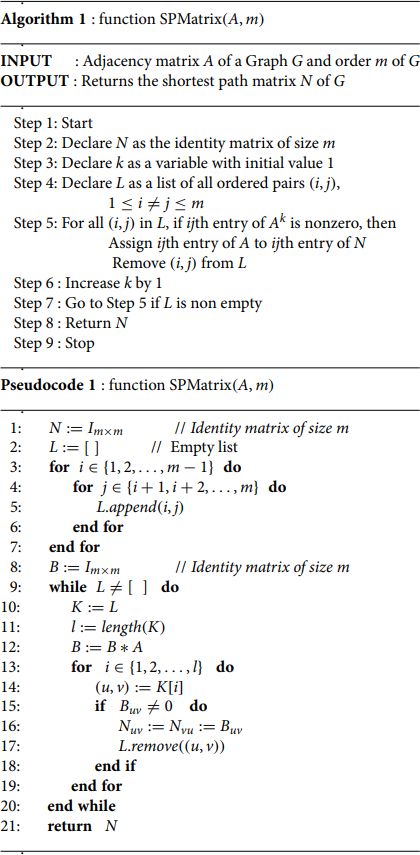

The $\mathbf{for}$ loops together in the steps 3 and 4 require $\frac{m(m-1)}{2}$ iterations. Matrix multiplication, is of $O(m^3)$ and the time required to execute the $\mathbf{for}$ loop in step 13 is at most $\frac{m(m-1)}{2}$, which is executed only if the list L is non empty. Considering the maximum possible iterations, i.e, considering the path graph, which requires $(m-1)$ iterations to make L an empty set, the total time required is less than $(m-1)[m^3+(\begin{array}{c}m\\ 2\end{array})+(\begin{array}{c}m-1\\ 2\end{array})+(\begin{array}{c}m-2\\ 2\end{array})+\dots +1]$. So it follows that the time complexity of Algorithm 1 is $O(m^4)+O(m^3)=O(m^4)$.

4.2 Stress of a vertex in general graph

The following Algorithm 2 returns the stress s of a given vertex $v_k$ of the graph.

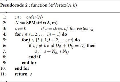
Initially to find the shortest path matrix in Step 2, we use the Algorithm 1. For m values of the $\mathbf{for}$ loop in Step 4 of Algorithm 2, the $\mathbf{for}$ loops in Step 6 and 7, will be executed in $(\begin{array}{c}m\\ 2\end{array})$ iterations. Total time required to execute these for loops will be $\left[\frac{m(m-1)}{2}\right]$. So the time complexity of Algorithm 2 will be $O(m^4)+O(m^2)=O(m^4)$.

4.3 Betweenness centrality of a vertex in general graph

With a slight variation in step 7 of Algorithm 2, here we present an algorithm to compute the betweenness centrality of a vertex.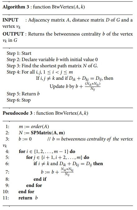

To find the shortest path matrix in step 2, we use the Algorithm 1 with complexity $O(m^4)$. Further, it requires $(\begin{array}{c}m\\ 2\end{array})$ iterations to run the $\mathbf{for}$ loops in step 4 and step 5. So the time complexity of Algorithm 2 will be $O(m^4)+O(m^2)=O(m^4)$.

4.4 Stress in Cartesian product

In the following Algorithm 3, we compute the stress of vertices in the Cartesian product of two graphs G and H. Algorithm 1 is used to get the shortest path matrix of G and H.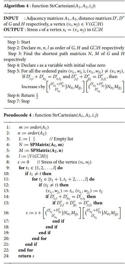

In the Algorithm 3, to find the matrices N and M in Steps 4 and 5, we use Algorithm 1 with complexity $O(m^4)+O(n^4)$. Further to execute the $\mathbf{for}$ loops in Steps 9 and 11, we require $(\begin{array}{c}l\\ 2\end{array})=(\begin{array}{c}mn\\ 2\end{array})$ iterations. Complexity will be $O(m^2{n}^2)$. So the time complexity of Algorithm 3 will be $O(m^4)+O(n^4)+O(m^2{n}^2)$. Without loss of generality, if we assume that $m\ge n$, then the time complexity of Algorithm 3 will be $O(m^4).$

4.5 Stress of vertices in a corona graph

In the following algorithm, we find the stress of vertices of $G°H$ using the adjacency matrices of G and H.

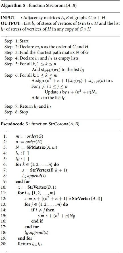
To find shortest path matrix of G in step 4, we use Algorithm 1 with complexity $O(m^4)$. In step 7, for n values, we use Algorithm 2 to find the stress of vertices in $u+H$. The complexity will be $O({(n+1)}^4)$ (where $n+1$ is the size of B). Algorithm 2 is used again in step 10 with complexity $O({(n+1)}^4)$. Further, for m values in the $\mathbf{for}$ loop in step 11, Algorithm 2 of complexity $O(m^4)$ will be used to calculate stress of vertex in G and the $\mathbf{for}$ loop in step 13 is executed m times. It follows that the complexity of this algorithm is $O(n^5)+O(m^5)$.

Acknowledgments

We thank Professor Bapat for bringing our attention toward number of paths between any two points on the chess board and its relation with binomial coefficient.

Disclosure statement

No potential conflict of interest was reported by the author(s).

Additional information

Funding

Among the authors, Manjunatha Prasad Karantha wish to acknowledge the funding support by Science and Engineering Research Board (DST), India through the projects CRG/2019/000238 and MTR/2018/000156.

References

- Borgatti, S. P., Everett, M. G. (2006). A graph-theoretic perspective on centrality. Soc. Netw. 28(4): 466–484.
- Bhargava, K., Dattatreya, N. N., Rajendra, R. (2020). On stress of a vertex in a graph. arXiv preprint arXiv:2208.13493.
- Camby, E., Caporossi, G., Paiva, M. H. M., Ribeiro, M. R. M., Segatto, M. E. V. (2018). On the number of shortest paths in Cartesian product graphs and its robustness. Les Cahiers du GERAD, GERAD, HEC Montreal, Canada.
- Harary, F. (1988). Graph Theory. Reading, AM: Addison-Wesley Publishing Company.
- Kumar, S., Kannan, B. (2020). Betweenness centrality in Cartesian product of graphs. AKCE Int. J. Graphs Comb. 17(1): 571–583.
- Lopez, R., Worrell, J., Wickus H., Florez, R., Darren, N. A. (2017). Towards a characterization of graphs with distinct betweeness centralities. Australas. J. Combin. 68(2): 285–303.
- Newman, M. (2018). Networks. Oxford: Oxford University Press.
- Poojary, R., Bhat, A. K., Subramanian, A., Karantha, M. P. (2023). The stress of a graph. Commun. Comb. Optim. 8(1): 53–65.
- Poojary, R., Bhat, A. K., Subramanian, A., Karantha, M. P. (2022). Stress of wheel related graphs. Natl. Acad. Sci. Lett. 45: 427–431.
- Scardoni, G., Laudanna, C. (2012). Centralities Based Analysis of Complex Networks. London: IntechOpen.
- Scardoni, G., Tosadori, G., Faizan, M., Spoto, F., Fabbri, F., Laudanna, C. (2015). Biological network analysis with CentiScaPe: Centralities and experimental dataset integration. F1000Research 3: 139.
- Shannon, P., Markiel, A., Ozier, O., Baliga, N. S., Wang, J. T., Ramage, D., Amin, N., Schwikowski, B., Ideker, T. (2003). Cytoscape: A software environment for integrated models of biomolecular interaction networks. Genome Res. 13(11): 2498–2504.
- Shimbel, A. (1953). Structural parameters of communication networks. Bull. Math. Biophys. 15(4): 501–507.