Road distance and travel time for an improved house price Kriging predictor

ABSTRACT

The paper designs an automated valuation model to predict the price of residential property in Coventry, United Kingdom, and achieves this by means of geostatistical Kriging, a popularly employed distance-based learning method. Unlike traditional applications of distance-based learning, this papers implements non-Euclidean distance metrics by approximating road distance, travel time and a linear combination of both, which this paper hypothesizes to be more related to house prices than straight-line (Euclidean) distance. Given that – to undertake Kriging – a valid variogram must be produced, this paper exploits the conforming properties of the Minkowski distance function to approximate a road distance and travel time metric. A least squares approach is put forth for variogram parameter selection and an ordinary Kriging predictor is implemented for interpolation. The predictor is then validated with 10-fold cross-validation and a spatially aware checkerboard hold out method against the almost exclusively employed, Euclidean metric. Given a comparison of results for each distance metric, this paper witnesses a goodness of fit () result of 0.6901 ± 0.18 SD for real estate price prediction compared to the traditional (Euclidean) approach obtaining a suboptimal value of 0.66 ± 0.21 SD.

KEYWORDS:

• Kriging
• Minkowski
• travel time
• road distance
• real-estate valuation

1. Introduction

By 2030, investable real estate is expected to have grown by more than 55%, amounting to a UK residential market value of £9.145 trillion (IPF 2017). Consequently, leaders of real estate, policy makers and everyday home buyers are looking for information-driven technological solutions to drive sustainable, low-risk decisions in a newly global market (PwC 2017). In addition, the complex network structures, unprecedented urban growth and wealth of available real estate data make (inter)national and urban residential markets more interesting and accessible than ever before. As such, machine-learning algorithms, under the name of automated valuation models (AVMs), exploit these data to reliably understand the value of real estate over large areas where market behavior may differ significantly. One such way to model these market behaviors is to utilize the vast data sources available to a single influential variable which in this case is space.

In view of the above, spatial relationships must be inferred differently to conventional (nonspatial) statistical models, most notable by the removal of the assumption of independent and identically distributed (IID) random variables. This is due to dependencies between spatial points, known as spatial autocorrelation (SAC). An occurrence of dependency structures in spatial data introduces redundancy that must be taken into account to avoid overestimation of statistical effects. As such, an experimental variogram is a means of computing spatial dependencies and continuity (Matheron 1963). Given the experimental variogram and the fact that spatial data have a stationary covariance, the variance for each omnidirectional pairwise distance is calculated. Thereafter, it is usual to fit a parametric model, known as the fitted variogram, to infer the topic in question using a regression, most commonly Kriging (Cressie 1988).

Inappropriately, the typical experimental variogram computes each pairwise distance with a Euclidean function (also called “as-the-crow-flies”). The Euclidean function is unrealistic for some (notably urban) settings which contain complex physical restrictions and social structures for example road and path networks, large restricted areas of private land and legal road restrictions such as speed limits and one-way systems. This paper hence hypothesizes that the “actual” space represented in the experimental (Euclidean) variogram is currently ill-informed. As such, we implement three new distance metrics into a set of house price Kriging predictors: (1) approximate road distance, (2) approximate travel time and (3) a combination of both.

Probably, the key reason for a small uptake in distance matrix optimization is due to the fact that one must ensure a valid positive definite covariance and conditionally negative definite variogram which cannot be guaranteed with any non-Euclidean distance functions (Curriero 2005, 2006). For this reason, nonmetric pairwise road distance and travel time matrices are highly unlikely to produce a valid variogram and covariance function. This puts forth a set of valid Minkowski distance metrics which are proven to better approximate restricted road distance and travel time across the Coventry (United Kingdom) road network compared with a Euclidean distance. Each result is compared with a set of popularly employed validation metrics (1) , (2) root mean squared error (RMSE) and (3) mean absolute percentage error (MAPE) on two validation sampling techniques (1) 10-fold cross-validation and (2) checkerboard holdout.

The key contributions of this paper are (1) a Minkowski approximation of a pairwise restricted road distance metric utilizing OpenStreetMap (OSM); (2) a Minkowski approximation of a pairwise travel time metric utilizing OSM; (3) a Minkowski approximation of a pairwise combined restricted road distance and travel time metric utilizing OSM; (4) a comparison study of house price predictors in Coventry with distance metrics (1)–(3) against a commonly used Euclidean metric. The final contribution shows that spatial interpolation can be improved with non-Euclidean distance functions.

Section 2 reviews related literature, Section 3 explores the open and crowd sourced data utilized to build a house price training set with road distance and travel time distance metrics. Section 4 describes the method offered by this paper in four stages: collapsing time, distance matrix estimation, variogram fitting and spatial interpolation. Afterward, Section 5 validates the procedure undertaken on a set of 3669 real-estate transactions across Coventry. Sections 6 discusses the scientific novelty and impact of this work. Finally, Section 7 concludes the paper with some discussions regarding further work opened up by this research.

2. Background reading

Most contemporary machine-learning-based AVMs are hedonic in nature (a function of multiple attributes) (Nelson 1999; McClusky and Borst 2007). Examples of such attributes relating to residential property pricing include topography and natural geography (Kok, Monkkonen, and Quigley 2011), building footprint (Pace et al. 1998), school proximity (Machin and Gibbons 2003), over head pylons (Bond, Sims, and Dent 2013) and crime (Thaler 1978). However, it has been shown that space (Crosby et al. 2016) and time (Huang, Wu, and Barry 2010) can best infer (up to 71% of) a property’s value (see Section 2.1). This paper attempts to inform each hedonic AVM by considering how to model space better.

2.1. House prices in space

Since the early nineteenth century, space and distance have been theorized as the primary functions for property valuation. For example, favored prices are given to those properties within close proximity to its central market place (Thunen 1826), community center (King 1984) or central business district (Caplin et al. 2008). Most contemporary analysis mimics this trend, for example predicting property value by using (1) the average sales price of other properties in the local comparable markets, (2) a spatial clustering of properties and demographics (Malczewski 2004) and (3) a local demographic “trade area” (Daniel 1994).

With regards to machine learning, Pace et al. (1998) describes the implementation of a spatiotemporal autoregressive model on 70,822 properties in Fairfax county from 1961 to 1991. Their prediction, with 12 variables, reduced the median absolute error by 37.35% relative to an indicator-based model. In addition, Crosby et al. (2016) uses a space only house price Kriging predictor to produce an of 0.72 on a nationwide UK AVM. Finally, Huang, Wu and Barry (2010) put forth a geographically and temporally weighted regression for house price prediction, in which an of 0.88 is achieved on a dataset of residential house sales in Calgary (Canada) between 2002 and 2004.

All aforementioned machine-learning approaches consider cross-validation sampling to estimate the generalizability of each model. In the case of spatially dependent data, cross-validation is optimistic due to its inherent IID assumption. As a result, we shall consider a cross-fold-validation for comparison against other work but also a spatially aware checkerboard hold out approach (defined in Section 5). Additionally, Euclidean distances are exclusively considered in all of the above work. This paper hypothesizes that house prices are related to a more complex structural network relating to (restricted) road distance and travel time; hence, we introduce an approximate (restricted) road distance and travel time metric using the Minkowski distance function for a valid house price Kriging predictor (Matheron 1963; Cressie 1990).

2.2. Non-Euclidean distance-based predictors

Manhattan (Ganio, Torgersen, and Gresswell 2005; Theodoridou et al. 2015), Geodetic (Banerjee 2005) and water-based (shortest path over water) (Murphy et al. 2014) distances have all been implemented in distance-based learning algorithms, each showing some minor improvements compared with the Euclidean function. Each of these methods is motivated by some access-restricted environment: city-based routing, world distances and smooth edges, respectively. In addition, this paper hypothesizes that road distance and travel time are intrinsic to contemporary house price modeling, and it is these features that we approximate.

Without direct access to the above datasets, it cannot be confirmed that the input metrics (Manhattan, geodetic or water-based) produce a valid variogram. As such, Curriero (2006) discusses dimensionality reduction to approximate a Euclidean metric from a (potentially invalid) non-Euclidean metric input. Using simulated data with isotropic spatial dependence, their work builds four omnidirectional variogram estimators, showing their newly defined “stream” distances consistently outperform the standard Euclidean function, whilst remaining always valid.

Similarly, Zou et al. (2012) produce a Kriging predictor with a road distance network using an Isomap algorithm, a variation of isometric embedding. The predictor estimates traffic flow in Nanchang, China. This method uses the Floyd Warshall algorithm to build a nonrestricted road network. This does not consider accessibility restrictions such as one-way systems or traffic lights.

Furthermore, Shahid et al. (2009) approximate the distance between a set of postcodes and a hospital with a 1 × N vector of Minkowski distances with the p value which is most correlated with the shortest path along the Calgary road network. The results from their paper motivate the experiment in this paper; however, we uniquely introduce an N × N distance matrix with a Minkowski p value most correlated to travel time, restricted road distances and a combination of both.

Finally, a Minkowski distance metric is also put forth with geographically weighted regression (GWR) (Lu et al. 2016). Their work tests GWR with a combination of Minkowski p values (1–8, ) at intervals of 0.25. This paper uses intervals of p = 0.05. This paper puts forward the interesting point that, for each dataset, a new p value may need to be calculated, which can be time consuming on large datasets. Notably, both GWR and Kriging are local–spatial prediction models; however, Kriging prediction is regularly noted as an improvement to GWR when validated (Matkan et al. 2010; Meng 2014).

3. Data description

Routing data are provided by the open street routing machine (OSRM), an open source routing engine for shortest paths in road networks for cars, bicycles and walking, supported by OSM. For example, Figure 1(a–c) shows a comparison of Euclidean distances between 0 and 4 mi, travel time between 0 and 10 min and road distance between 0 and 4 miles.

Figure 1. A comparison of an Euclidean distance matrix versus a drive time distance matrix and a road distance matrix around the center point of Coventry. (a) Euclidean distance buffer from 0 to 4 miles around the centre of Coventry; (b) Travel time distance buffer from 0 to 10 minutes drive time around the centre of Coventry; (c) Road distance buffer from 0 to 4 miles around the centre of Coventry.

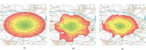
The diagrams show how restrictions can alter the lag between points in a real estate predictor. In addition, Table 1 provides a description of all restrictions considered. The residential sold price data are sourced from Her Majesty’s land registry’s openly available “Price Paid” database. These data are space and time stamped for all residential properties that have been sold in England and Wales since 1995. All freehold houses between 1 January 2016 and the 1 January 2017 in the city of Coventry are used. Additionally, Ordnance Survey (OS) offers an educationally available dataset containing all the address locations in the United Kingdom. Table 2 provides a name, description and data type for all key data utilized.

Table 1. All restrictions to road network and travel time OSRM calculation from OSM labels.

Restriction type	Description
Barrier	(Rising) bollard, cattle grid, border control, checkpoint, toll booth, sally port, (lift) gate etc.
Restriction	Motor vehicle, vehicle, permissive, designated, destination, private, agricultural, forestry, emergency, parking aisle etc.
Speed profile	Motorway, trunk, primary, secondary, tertiary, ferry, residential, living street, track, unclassified etc.
Surface speeds	Concrete, paved, cement, compacted, paving stones, metal, grass, gravel, unpaved, cobblestone, stone, sand, mud etc.
Tracktype speeds	Grade 1–5, intermediate, bad, horrible, impassable etc.
Maxspeed	Urban, rural, trunk, motorway, single/dual carriageway
U-Turn	Time in seconds
Traffic signal	Time in seconds
Oneway	Boolean, y/n
Route speed	Ferrys, piers, movable bridges

Table 2. Feature name, description and data type in HMLR’s Price Paid dataset.

Feature name	Description	Data type
UID	Unique transaction identifier	Integer
Property type	Flat, terraced, semi-detached, detached	String
Tenure	Freehold or leasehold	Binary
Date of transaction	Transaction date for the property	Date/Time
Address	Full address including postcode	String
Build status	Is the property newly built	Binary

To ensure that these data contain the expected SAC required for successful hypothesis testing, the standard Moran’s I-test is considered:

(1)

where  = observations,  = distance weightings,  = total number of observations,  =  and is the mean of . If , then the values at location are positively autocorrelated, else negatively correlated.

As expected, the houses dataset (containing 3669 properties) showed a strong result of , also showing a standard deviation of and value . These results allow us to reject the null hypothesis that there is no SAC present at significance level  = . These results emphasize the appropriateness of spatial interpolation.

4. Scientific method

Given that house prices contain some spatial relationships, we undertake prediction on all houses sold in Coventry. This paper introduces a multiple stage approach. The first stage converts a discrete, nonuniform, spatiotemporal sold price dataset into a uniform time singular sold price output utilizing a space–time comparable process in Coventry. Stage 2 attempts to utilize Minkowski coefficients to predict the road distance and travel time values for all pairwise house price points. Finally, stage 3 builds a set of variograms for each distance metric and stage 4 implements ordinary Kriging to identify a new feature of spatial dependencies related to real-estate prices. The resulting model is trained on a sample of 3669 instances and is validated against five distance metrics (Euclidean, Manhattan, road distance, travel time and a combination) using 10-fold cross-validation and checkerboard hold out. Algorithm 1 provides the pseudo-code for our entire experiment.

Table

Algorithm 1: Collapsing time distance matrix selection variogram parameter selection spatial interpolation.
Required: , , , maximum likelihood estimator (MLE)
1: Input:
2: Temporal mapping to time :
3:
4: Stratified sampling: Sample across each LSOA
5:
6: for z in {road distance, travel time, linear combination} do
7: =
8: for z in {road distance, travel time, linear combination} do
9:for V in 10-folds, Checkerboard do
10: Variogram selection on vs ← MLE (
11: Ordinary Kriging on  (
12: return
13: Finish

4.1. Stage 1: collapsing time

The price paid data for 2016 are addressed only (herewithin named ). This accounts for 3669 sales in Coventry. Stage 1 predicts each property’s sale price based on its value on the 1 January 2017 (for time singularity). This process involves each property being assigned some percentage price change based on the date that it was sold and the lower super output area that the property is contained within to produce a value for all 3669 properties at the date 1 January 2017 (). The error for the purposes of this experiment is minimal or nonexistent due to the small temporal and spatial aggregate areas being considered.

4.2. Stage 2: distance matrix estimation

Consider a list of points {} in a Euclidean space of dimension . A matrix is called a Euclidean distance metric such that are the pairwise distances between all other points and (. Hence, all must satisfy each of the four distance metric properties such that

(P1: Non-negativity)

(P2: Self-distance)

(P3: Symmetry)

(P4: Triangle inequality)

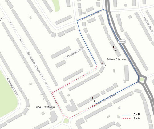
Although each property is necessary, they are not exclusively sufficient. The road distance example satisfies just some of these properties (P1, P2); however, it does not exclusively fulfill P3 or P4. A practical example would be to consider a one-way system in a city, whereby one route may be longer than its counterpart route. Figure 2 shows an exact example where the distance between houses to is 0.24 mi along the red dotted line which takes a route along “Brownshill Green Road” and is marked as a one-way system, this means that the route to must be different, which, in this case, is further; hence, the distance matrix is not symmetric. The same reasoning applies for a travel time matrix.

Figure 2. A situation where P3 and P4 are not satisfied.

A daily average distance and travel time is calculated to overcome changing patterns. With regards to producing a road distance and travel time matrix which satisfies P3 and P4, one must produce a matrix prediction. A simple method of making the distance matrix symmetric would be to duplicate the lower triangle, select the minimum or maximum of the lower/upper triangle or calculating the average between route A  B and B  A. However, this doesn’t always overcome the problem of P4 as a shorter nonrestricted route could potentially be found. The experiment of this paper instead considers Minkowski coefficients:

(2)

where and are the longitudinal and latitudinal points of each data point . Matrix has a p ≥ 1 as a result of the Minkowski inequality (Hardy, Littlewood, and Pólya 1952). Euclidean and Manhattan are special cases of p = 2 and p = 1, respectively. More specifically, it can be seen that Manhattan and Euclidean have several similarities, most notably that the Manhattan distance is always greater than or equal to Euclidean distance and that when reduced to a one-dimensional state, Manhattan is exactly Euclidean unlike any other values of p which shows the significance of these special cases. Assuming that there is a Minkowski p value that is similar to road distance, travel time or a combination of both, then this Minkowski value can be used as a valid estimate of road distance and/or travel time.

Estimation optimization

For this experiment, three scenarios are attempted:

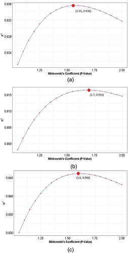
(1) find the Minkowski p value with the highest value to the actual road distance matrix (p = 1.55),

(2) find the Minkowski p value with the highest value to the actual travel time matrix (p = 1.7) and

(3) find the Minkowski p value with the highest value to the actual road distance matrix and travel time matrix using linear regression (p = 1.6).

Figure 3 shows the value for each Minkowski p at 0.05 intervals between 1 (Manhattan) and 2 (Euclidean). It can be seen that a combination of the two distance matrices has the highest  =  value at , which shows that Minkowski coefficients are capable of predicting a realistic urban environment with a road network, much better than Euclidean or Manhattan distance matrices.

The combined road distance and travel time matrix is calculated as a linear model with four variables: (1) road distance A  B, (2) road distance B  A, (3) travel time A  B, (4) travel time B  A. This is an approach which to our knowledge has never before been undertaken and attempts to fully understand the utility function of a house purchaser. Fig 4 provides a comparison of each physical distance (Euclidean, Manhattan, actual road [in both directions] and optimal Minkowski estimate) between two points.

Figure 3. The goodness of fit value for each Minkowski coefficient tested against the OSRM’s actual road distance calculations, travel time calculations and a linear model of both (here embedded R² = r², and P-Value = p-value). (a) OSRM road distance versus Minkowski p-value goodness of fit graph; (b) OSRM travel time versus Minkowski p-value goodness of fit graph; (c) OSRM linear combination of road distance and travel time versus Minkowski p-value goodness of fit graph.

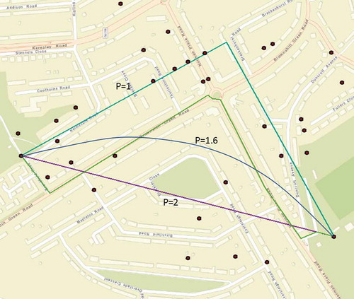
Figure 4. A streetmap comparing the distances: the road distance, the Euclidean distance, the Manhattan distance and the Minkowski estimated distance.

4.3. Stage 3: variogram fitting

For comparison, we test all of the highly correlated Minkowski p values () against each scenario (road distance, travel time and a combination). Let’s assume a set of spatial locations (i.e. longitudinal and latitudinal points) such that are known and that is a real valued stochastic process over random fields. For one to predict some value (house prices) at location from observed values , they must first ensure that the data represent a complete sampling of a single realization such that

(3)

and

(4)

A function which assumes Equations 3 and 4 is called second-order stationary. Suppose a function is the semivariogram and that the data have a stationary covariance, then the semivariance is related to the covariance function with a nugget, sill and range (Cressie 1988).

With this in mind, the covariance function is estimated, by fitting a parametric model to the calculated semivariance utilizing least squares. This function assumes that the semivariance of the data can be modeled. The process ran 5 times, one for each distance matrix. The different distance matrices alter the semivariance of the data such that the lag for each point is always greater than or equal to a Euclidean matrix but not consistently or linearly greater than or equal to; hence, the semivariance for each spatial lag will alter with each distance matrix. This is due to the fact that the estimated variogram model and parameters, which are a function of distance, will differ as the distance between each value does too. Noting the results in Section 6, it is not surprising to find that the same model (Matern) is optimal in all cases because each distance matrix used to plot the lag is highly correlated. The Matern model is

(5)

where is the gamma function; is the modified Bessel function of the second kind, and and are non-negative parameters of the covariance. The best parameters use maximum likelihood estimates (MLE) for random fields that are satisfied through Equations 3 and 4.

4.4. Stages 4: spatial interpolation

For this paper, we will consider ordinary Kriging only. Kriging is used to estimate the aforementioned values (), based on the surrounding existing values () such that is an equation of coefficients each multiplied by their respective value . In the case of ordinary Kriging, variogram values show the relationship between the, in our case, house price data and the point of interest ().

(6)

This equation is required such that it is unbiased and minimizes the mean squared error, which when minimized is

(7)

where is the Lagrangian multiplier used to ensure . Hence, ordinary Kriging assumes a constant mean of the underlying real-valued random function . The Kriging variance is simply minimized by using as defined above. We calculate five variograms for prediction comparison (restricted road distance, travel time, Euclidean, Manhattan and combined road distance and travel time).

5. Cross-validation and validation metrics

Cross-validation splits the dataset into two subsets: a training set where a model is fitted on and a validation test set where the model is evaluated on (Stone 1974). The main purpose of cross-validation is to detect over fitting and estimate how well a model will generalize to unseen data. k-Fold cross-validation is the most popular method, in which data are partitioned into k subsets, performs the analysis on k − 1 subsets (training) and validates the analysis on the remainder. The process is repeated k times where the test set is different each time. The validation results between each fold are averaged to reduce outlier bias (Kohavi 1995). Given the popularity of k-fold cross-validation, we apply the method with 10-folds.

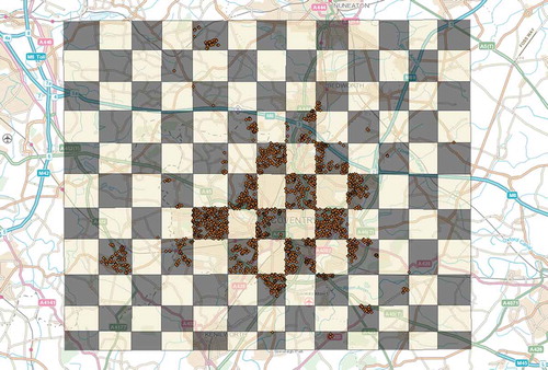
k-Fold cross-validation, on the other hand, can be inappropriate in a spatial setting due to its inherent IID assumption which is violated by spatial dependency. As such, we also put forth an alternative method which attempts to take account for some of the spatial dependencies in house price data known as stratified checkerboard holdout. This method provides a training sample of 1832 properties and test sample of 1837 properties. Figure 5 shows the checkerboard polygons used to separate the training and validation test set for each experiment. This method attempts to provide a more realistic estimation of the models generalization performance; however, it contains a smaller training set, which may provide pessimistic results. In addition, the training and test data contain SAC at the checkerboard borders; so, this method does not fully remove the spatial dependency.

Figure 5. Spatially aware checkerboard sampling utilized in the validation process to confirm the model is not over fitted.

The experiment’s success is measured on a number of validation metrics: (1) , (2) RMSE and (3) MAPE. A paired T-test is also undertaken to state whether the results are statistically significant enough for the null hypothesis that the price of a house can be predicted by space only.

The calculation measures the predictor’s ( “goodness of fit” [the model’s ability to fit the test data ()]):

(8)

The RMSE intuitively takes the square root of the sum of the mean squared errors:

(9)

MAPE is the mean absolute error, expressed as a percentage:

(10)

The paired T-test shows whether the mean of a population of predicted data-points (i.e. predicted house prices) differs significantly from the mean of the actual population. This is calculated as the ratio of signal to noise such that

(11)

where and are the mean values of the predicted dataset and the actual data set, respectively. Finally, the p value compares our value with that of the Student T distribution with degrees of freedom. The smaller the p value, the more statistically significant the model is deemed to be.

6. Results

This paper applied ordinary Kriging five times, each fitted with a variogram exploiting Minkowski predictions used to simulate a more appropriate valuation environment. Tables 3 and 4 provide the validation results for each model showing that non-Euclidean distance metrics can produce a more appropriate set of parameters for house price prediction in Coventry. For example, the best performing model utilizes a linear regression of OSRM’s road distance and travel time in both directions.

Table 3. Results for 10-fold cross-validation.

	10-fold cross-validation
Distance matrix	= 1 (Manhattan)	= 1.55	= 1.6	= 1.7	= 2 (Euclidean)
	0.683	0.6847	0.6901	0.6843	0.663
RMSE	57,115	57,000	57,013	57,439	58,913
MAPE	17.92%	17.9%	17.895%	18.01%	18.12%

Table 4. Results for checkerboard holdout.

	Checkerboard stratified validation
Distance matrix	= 1 (Manhattan)	= 1.55	= 1.6	= 1.7	= 2 (Euclidean)
	0.4509	0.4514	0.4558	0.4499	0.4418
RMSE	82,414	82,367	81,940	82,507	82,972
MAPE	24.52%	24.51%	24.40%	24.53%	24.57%

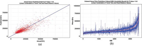
In assessing Tables 3 and 4, it can be seen that a Minkowski p of 1.6 is consistently the best performing and Euclidean is the least. Figure 6(a) visualizes the prediction versus actual price for all properties trained with our best performing distance matrix (p = 1.6). In addition, Figure 6(b) shows the uncertainty bounds between folds for all properties in the price paid dataset. The best performing models T-value and P-value are reported to be 1.312 and 0.1896, respectively, showing that space as a single variate is weak on its own; some more covariates could really support the model. In general, the results show that residential valuation has a relatively strong SAC which, with the use of appropriate distance metrics, can be improved. In addition, a Students’s T-test between experiments is calculated to show that the best performing (p = 1.6) and poorest performing (Euclidean) Kriging outputs provide a statistically significant improvement with a P value of 0.0458. This is an appropriate test because the two populations have very similar (almost equal) variances (86,555 and 86,657, respectively).

Figure 6. Validation diagrams: (a) the actual versus predicted graph and (b) house price prediction graph with uncertainty bounds both with a Minkowski coefficient of p = 1.6.

7. Conclusion

This research has (1) converted a discrete, nonuniform, spatiotemporal sold price dataset into a uniform time singular sold price output utilizing a space–time comparable process in Coventry; (2) deployed a novel method of N × N road distance and travel time predictions; (3) built five variograms, each with a different distance function; (4) produced a spatially aware ordinary Kriging calculation identifying house price spatial dependencies. In addition, each of the models is tested using MAPE, RMSE and yielding an adjusted value of 0.69 compared with the traditional Euclidean approach at 0.66. Future work is to include (1) testing the hypothesis with other applications and spatial interpolation methods; (2) implementing the findings into the space, property, economic, network and time algorithm from Crosby et al. (2016); and (3) introducing a set of covariates.

Acknowledgments

We would like to thank members of the SIGSpatial community whose previous feedback led to this contribution. Additionally, we would like to convey our gratitude to the attendees of the workshop on Spatial Urban Analytics and Crowdsourced Geographic Information for Smarter Cities, associated with the RGS-IBG Annual International Conference 2017. Finally, our appreciation goes to all of the open-source mapping contributors out there.

Additional information

Funding

This work was supported by the Engineering and Physical Sciences Research Council (EPSRC) Centre for Doctoral Training in Urban Science: [Grant Number EP/L016400/1] and Assured Property Group. This work was also supported by The Alan Turing Institute: [Grant Number EP/N510129/1] and the Lloyd’s Register Foundation programme on Data Centric Engineering.

Notes on contributors

Henry Crosby

Henry Crosby is a PhD candidate at the Centre for Doctoral Training in Urban Science in the Warwick Institute for the Science of Cities. He received his BSc(Hons) degree in Business and Mathematics from Aston University, United Kingdom, and his MSc in data analysis at the University of Warwick.

Theo Damoulas

Theo Damoulas is an associate professor in Data Science with a joint appointment in the Department of Statistics and Department of Computer Science at the University of Warwick. He is also a Turing Fellow of the Alan Turing Institute and affiliated with NYU as a visiting exchange professor at the Center for Urban Science and Progress (CUSP). Previously, he was a research associate at Cornell University. His studies were undertaken at the University of Edinburgh, Manchester and Paul Scherrer Institut, Switzerland.

Alex Caton

Alex Caton is a PhD candidate at the Centre for doctoral training in Urban Science in the Warwick Institute for the Science of Cities and Alex Caton has a BSc(Hons) in Discrete Mathematics as well as an MSc in Urban Informatics and Analytics, both from the University of Warwick.

Paul Davis

Paul Davis is the co-owner and chief technology officer of Nimbus Maps – the most comprehensive and powerful property intelligence tool in the United Kingdom. Nimbus Maps is the essential “property dating platform” for the real estate industry utilized by agents, asset managers, developers, lawyers, investors and property companies.

João Porto de Albuquerque

João Porto de Albuquerque studied at the University of Campinas, Brazil, and Technical University of Dortmund, Germany. He conducted postdoctoral research in social studies of information systems at the University of Hamburg, Germany, and then acted as a visiting professor at the Institute of Geography of Heidelberg University. He also worked at the School of Arts, Sciences and Humanities of the University of São Paulo (2008–2010) and at the Department of Computer Systems at the University of São Paulo (2010–2015), Brazil. Now, he is an associate professor at the Centre for Interdisciplinary Methodologies and codirector of the Warwick Institute for the Science of Cities.

Stephen A. Jarvis

Stephen A. Jarvis studied at London, Oxford and Durham Universities before taking his first lectureship at the Oxford University Computing Laboratory. After a short secondment to Microsoft Research in Cambridge, he joined the University of Warwick, rising to professor in 2009. He acted as Director of Research from 2008 to 2013 at which point he was appointed chair of department. Professor Jarvis is a visiting exchange professor at New York University and is engaged with the Alan Turing Institute. He is presently deputy pro vice chancellor (research) at the University of Warwick.

References

- Banerjee, S. 2005. “On Geodetic Distance Computations in Spatial Modeling.” Biometrics 61 (2): 617–625. doi:10.1111/biom.2005.61.issue-2
- Bond, S., S. Sims, and P. Dent. 2013. Towers, Turbines and Transmission Lines: Impacts on Property Value. Chichester, UK: Wiley-Blackwell.
- Caplin, A., S. Chopra, J. V. Leahy, Y. LeCun, and T. Thampy. 2008. “Machine Learning and the Spatial Structure of House Prices and Housing Returns.” doi:10.2139/ssrn.1316046
- Cressie, N. 1988. “Spatial Prediction and Ordinary Kriging.” Mathematical Geology 20 (4): 405–421. doi:10.1007/BF00892986
- Cressie, N. 1990. “The Origins of Kriging.” Mathematical Geology 22 (3): 239–252. doi:10.1007/BF00889887
- Crosby, H., T. Damoulas, P. Davis, and S. A. Jarvis. 2016. “A Spatio-Temporal, Gaussian Process Regression, Real-Estate Price Predictor.” Vol. The 24th ACM SIGSPATIAL International Conference on Advances in Geographic Information Systems, Burlingame, California, October 31 November 03., 68. ACM.
- Curriero, F. 2005. “On the Use of Non-Euclidean Isotropy in Geostatistics.” https://biostats.bepress.com/jhubiostat/paper94/
- Curriero, F. 2006. “On the Use of Non-Euclidean Distance Measures in Geostatistics.” Mathematical Geology 38 (8): 907–926. doi:10.1007/s11004-006-9055-7
- Daniel, L. 1994. “GIS Helping to Reengineer Real Estate.” Vol. 3. https://www.colorado.edu/geography/gcraft/notes/gisapps/reengr.html
- Ganio, L., C. Torgersen, and R. Gresswell. 2005. “A Geostatistical Approach for Describing Spatial Patterns in Stream Networks.” Frontiers in Ecology and the Environment 3 (3): 138–144. doi:10.1890/1540-9295(2005)003[0138:AGAFDS]2.0.CO;2
- Hardy, G., J. Littlewood, and G. Pólya. 1952. Inequalities. Cambridge: Cambridge University Press.
- Huang, B., B. Wu, and M. Barry. 2010. “Geographically and Temporally Weighted Regression for Modeling Spatio-Temporal Variation in House Prices.” International Journal of Geographical Information Science 24 (3): 383–401. doi:10.1080/13658810802672469
- IPF. 2017. “The Size and Structure of the UK Property Market: End-2016 Update.” http://www.ipf.org.uk/resourceLibrary/the-size-and-structure-of-the-ukproperty-marketyear-end-2016-update-july-2017-full-report.html, July.
- King, L. J. 1984. Central Place Theory. Beverly Hills, CA: Sage Publications.
- Kohavi, R. 1995. “A Study of Cross-Validation and Bootstrap for Accuracy Estimation and Model Selection.” The 14th international joint conference on artificial intelligence, Montreal, Canada, August.
- Kok, N., P. Monkkonen, and J. Quigley. 2011. “Economic Geography, Jobs, and Regulations: The Value of Land and Housing.” http://gspp.berkeley.edu/research/working–paper–series/economic–geography–jobs–and–regulations–the–value–of–land–and–housing
- Lu, B., M. Charlton, C. Brunsdon, and P. Harris. 2016. “The Minkowski Approach for Choosing the Distance Metric in Geographically Weighted Regression.” International Journal of Geographical Information Science 30 (2): 351–368. doi:10.1080/13658816.2015.1087001
- Machin, S., and S. Gibbons. 2003. “Valuing School Quality, Better Transport, and Lower Crime: Evidence from House Prices.” Oxford Review of Economic Policy 24 (1):99–119. 2008.
- Malczewski, J. 2004. “GIS-based Land-Use Suitability Analysis: A Critical Overview.” Progress in Planning 62 (1): 3–65. doi:10.1016/j.progress.2003.09.002
- Matheron, G. 1963. “Principles of Geostatistics.” Economic Geology 58 (8): 1246–1266. doi:10.2113/gsecongeo.58.8.1246
- Matkan, A., A. Shakiba, B. Mirbagheri, and H. Tavoosi. 2010. “A Comparison between Kriging, CoKriging and Geographically Weighted Regression Models for Estimating Rainfall over North West of Iran.” 10th EMS Annual Meeting, 8th European Conference on Applications of Meteorology (ECAM) Abstracts, Zürich, Switzerland, September. 13–17, 2010. http://meetings.copernicus.org/ems2010/, id. EMS2010–325.
- McClusky, W., and R. Borst. 2007. “Specifying the Effect of Location in Multivariate Valuation Models for Residential Properties.” Property Management 25: 312343.
- Meng, Q. 2014. “Regression Kriging versus Geographically Weighted Regression for Spatial Interpolation.” International Journal of Advanced Remote Sensing and GIS 3 (1): 606.
- Murphy, R., E. Perlman, W. Ball, and F. Curriero. 2014. “Water-Distance-Based Kriging in Chesapeake Bay.” Journal of Hydrologic Engineering 20 (9): 05014034. doi:10.1061/(ASCE)HE.1943-5584.0001135
- Nelson, A. 1999. “Transit Stations and Commercial Property Values: A Case Study with Policy and Land-Use Implications.” Journal of Public Transportation 2 (3): 77–95. doi:10.5038/2375-0901.2.3.4
- Pace, R. K., R. Barry, J. M. Clapp, and M. Rodriquez. 1998. “Spatiotemporal Autoregressive Models of Neighborhood Effects.” The Journal of Real Estate Finance and Economics 17 (1): 15–33. doi:10.1023/A:1007799028599
- PwC. 2017. “Real Estate 2020 Building the Future.” https://www.pwc.com/gx/en/industries/financial-services/asset-management/publications/real-estate-2020-building-the-future.html
- Shahid, R., S. Bertazzon, M. Knudtson, and W. Ghali. 2009. “Comparison of Distance Measures in Spatial Analytical Modeling for Health Service Planning.” BMC Health Services Research 9 (1): 200. doi:10.1186/1472-6963-9-200
- Stone, M. 1974. “Cross-Validation and Multinomial Prediction.” Biometrika 61 (3): 509–515. doi:10.1093/biomet/61.3.509
- Thaler, R. 1978. “A Note on the Value of Crime Control: Evidence from the Property Market.” Journal of Urban Economics 5 (1): 137–145. doi:10.1016/0094-1190(78)90042-6
- Theodoridou, P., G. Karatzas, E. Varouchakis, and G. Corzo Perez. 2015. “Geostatistical Analysis of Groundwater Level Using Euclidean and Non-Euclidean Distance Metrics and Variable Variogram Fitting Criteria.” In The EGU General Assembly Conference (Abstracts), Vienna, Austria, April 12–17, Vol. 17.
- Thunen, J. 1826. Der Isolierte Staat in Beziehung Auf Landwirtschaft Und Nationalkonomie, Hamburg, Perthes. Oxford: Oxford University Press.
- Zou, H., Y. Yue, Q. Li, and A. G. O. Yeh. 2012. “An Improved Distance Metric for the Interpolation of Link-based Traffic Data Using Kriging: A Case Study of a Largescale Urban Road Network.” International Journal of Geographical Information Science 26 (4): 667–689. doi:10.1080/13658816.2011.609488