Toward a unified theoretical framework for photogrammetry

ABSTRACT

The objective of photogrammetry is to extract information from imagery. With the increasing interaction of sensing and computing technologies, the fundamentals of photogrammetry have undergone an evolutionary change in the past several decades. Numerous theoretical progresses and practical applications have been reported from traditionally different but related multiple disciplines, including computer vision, photogrammetry, computer graphics, pattern recognition, remote sensing and machine learning. This has gradually extended the boundary of traditional photogrammetry in both theory and practice. This paper introduces a new, holistic theoretical framework to describe various photogrammetric tasks and solutions. Under this framework, photogrammetry is generally regarded as a reversed imaging process formulated as a unified optimization problem. Depending on the variables to be determined through optimization, photogrammetric tasks are mostly divided into image space tasks, image-object space tasks and object space tasks, each being a special case of the general formulation. This paper presents representative solution approaches for each task. With this effort, we intend to advocate an imminent and necessary paradigm change in both research and learning of photogrammetry.

KEYWORDS:

• Photogrammetry
• reverse imaging
• optimization
• computer vision

1. Introduction

Photogrammetry is the science and technology of extracting reliable three-dimensional geometric and thematic information, often over time, of objects and scenes from image and range data (Chen et al. 2016). Its objective is to extract various information from imagery. After over 150 years development, photogrammetry has approached to digital photogrammetry through plane-table photogrammetry, analog photogrammetry and analytical photogrammetry (Schenk 2005). Images of an interested scene or object are the primary input data for photogrammetry. With the rapid advancement and interaction of sensing and computing technologies, the spatial resolution of cameras and the computing power of computers have increased tremendously. As such, more subject areas and applications in image-based science have emerged, such as image segmentation, simultaneous localization and mapping (SLAM), point cloud generation, mesh generation and 3D modeling, where the tasks of photogrammetry are not limited to, and extended beyond, generating Digital Elevation Model (DEM), Digital Orthophoto Map (DOM), Digital Line Graph (DLG) or other traditional surveying products (Li, Zhu, and Li 2000b; Li 2000a).

Theories of traditional photogrammetry focused on topographic applications are facing many intrinsic limitations and challenges. Sensors we are using are extended from metric cameras to uncalibrated, off-the-shelf ones, from a single sensor to sensor systems (Shan 2017). Assumption of vertical photography and the subsequent approximate analytics do not hold any further or need extension for ever popular oblique and multi-view images. Our interest is extending from natural surface, which is usually continuous, to man-made objects, which are not continuous. Such change challenges many of the existing analytics in image matching, surface modeling and object reconstruction. In addition, multi-view imaging or indoor sensing would not allow us to deal with sensed targets as 2.5D any further (Real Ehrlich and Blankenbach 2019; Li and Fu 2018). Instead, mathematics of multi-valued functions become necessary (Boyd and Vandenberghe 2004). Finally, the use of multi-view images also raises the need to consider radiometric variations of the object surfaces (Wu et al. 2011), which has to be based on a framework that combines imaging geometry and imaging physics.

The imagery itself records both geometric and radiometric information of the object through a complicated imaging process. However, many applications in image-based science are only concerned with either geometric or radiometric information alone. For example, multi-view geometry (Brown, Burschka, and Hager 2003; Furukawa and Ponce 2009; Hirschmüller 2008) reconstructs the 3D object relying on the corresponding relations among different images but often neglects the radiometric process of imaging, whereas shape from shading (Horn 1970; Zhang et al. 1999; Kemelmacher-Shlizerman and Basri 2011) recovers the 3D shape of object according to the radiometric process of imaging without using the multi-view geometry. The quality of both tasks might be improved if the two types of information can be utilized in a complementary way. In addition, there is no systematic in-depth understanding about the relations of all the newly or conventional applications. As a result, it is necessary, to build a unified theoretical framework for photogrammetry to make full use of the information recorded in images, to clarify the concepts, and to understand the intrinsic relations of these tasks. To this end, we represent the process of imaging with one mathematical model and formulate all the photogrammetry tasks under this imaging model. According to the domain the tasks occur, the photogrammetric tasks are divided into image space tasks, image-object space tasks and object space tasks.

The paper is organized as follows. Section 2 describes the unified framework of photogrammetry. Sections 3–5 respectively explain the image space tasks, object-image space tasks and object space tasks. Section 6 summarizes the paper.

2. A unified framework

2.1 General expression of the imaging process

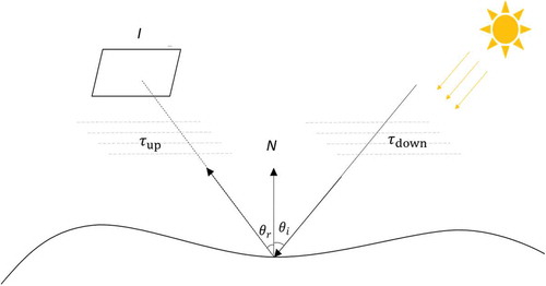
As shown in Figure 1, the physics of imaging involves five processes (Bakker et al. 2001; Peng, Zhang, and Shan 2015). The lighting process needs one or more light sources like the sun or skylight. Through the downward transmitting process, the photons from the light source transmit to the ground or object surface. The photons hit the surface and reflect. In the upward transmitting process, photons reflected from the surface transmit to the sensor through the atmosphere or other media. Finally, in the sensor response process, the camera translates the captured photons to image intensity with an analog-to-digital conversion.

Figure 1. Concept of imaging physics. $I$ is the image, $N$ is the normal of the object,${\tau }_{\mathrm{d}\mathrm{o}\mathrm{w}\mathrm{n}}$, ${\tau }_{\mathrm{u}\mathrm{p}}$ are the upwelling and downwelling transmitting process, ${\theta }_i,{\theta }_r$ are the incident angle and reflection angle, respectively.

Such imaging process can be described by the following mathematic expression

(1) $I\left(x,y\right)=h\left(\gamma ,c,{\tau }_{\mathrm{u}\mathrm{p}}\left(A_{\mathrm{u}\mathrm{p}},f\left({\tau }_{\mathrm{d}\mathrm{o}\mathrm{w}\mathrm{n}}\left(E,A_{\mathrm{d}\mathrm{o}\mathrm{w}\mathrm{n}}\right),\rho ,X,{\theta }_i,{\phi }_i,{\theta }_r,{\phi }_r\right)\right)\right)$(1)

where

• $I\left(x,y\right)$ is the image intensity of the image point $\left(x,y\right)$;

• $E$ is the energy of the light source;

• $\rho$ is the surface albedo;

• $X$ is the coordinates of the object which can represent the surface shape;

• $A_{\mathrm{u}\mathrm{p}}$ and $A_{\mathrm{d}\mathrm{o}\mathrm{w}\mathrm{n}}$ are the upwelling and downwelling atmosphere;

• ${\theta }_i$, ${\phi }_i$, ${\theta }_r$ and ${\phi }_r$ are the incident zenith, incident azimuth, reflection zenith and reflection azimuth, respectively;

• ${\tau }_{\mathrm{u}\mathrm{p}}$ and ${\tau }_{\mathrm{d}\mathrm{o}\mathrm{w}\mathrm{n}}$ are, respectively, the upwelling and downwelling transmitting process with the atmosphere $A_{\mathrm{u}\mathrm{p}}$ and $A_{\mathrm{d}\mathrm{o}\mathrm{w}\mathrm{n}}$;

• $f$ is the reflection function which describes the reflection process with the albedo $\rho$, surface shape (can be represented by surface coordinates $X$), incident angles and reflection angles in which the albedo depends on the material of the observed object and reflection angles are related to the camera setting. Usually, the reflection process is modeled using the Bidirectional Reflectance Distribution Function (BRDF);

• $h$ is the camera response function with the factor parameter $\gamma$ and camera parameter set $c$, which includes the interior and exterior orientation parameters.

It is noted we do not explicitly distinguish vectors or scalars as often times it is clear from the context. When dealing with close-range, oblique or aerial images, the influence of atmosphere $A_{\mathrm{u}\mathrm{p}}$ and $A_{\mathrm{d}\mathrm{o}\mathrm{w}\mathrm{n}}$ is often omitted and the incident zenith ${\theta }_i$, incident azimuth ${\phi }_i$, reflection zenith ${\theta }_r$ and reflection azimuth ${\phi }_r$ can be simplified to incident angle and reflection angle. The imaging process can then be simplified to the equation below:

(2) $I\left(x,y\right)=h\left(\gamma ,c,f\left(L,\rho ,X,{\theta }_i,{\theta }_r\right)\right)$(2)

Consequently, the simplified imaging process contains the illumination $L$, albedo of the surface $\rho$, the coordinates of the object $X$, incident angle ${\theta }_i$, reflection angle ${\theta }_r$ and camera parameter $c$.

2.2 Photogrammetry as reverse imaging

As mentioned above, the imaging process records the geometric and radiometric information of the interested object. The task of traditional photogrammetry is to recover the geometric information from the images, which is actually the reverse of such imaging process. For example, recovering the 3D position of the object is a typical reversed imaging process in which the unknown position of the object is estimated from the observed images with a standard procedure, including tie points matching, bundle adjustment, dense image matching and forward intersection (Wang 1990; Li, Wang, and Zhou 2008). The bundle adjustment helps to estimate the camera parameters including interior orientation parameters (focal length, principle point position and camera distortion) and exterior orientation parameters (camera locations and orientations) (Li and Shan 1989; Beardsley, Tort, and Zisserman 1996; Agarwal et al. 2010; Wu 2016; Shan 2018), whereas the corresponding 3D coordinates of the object are determined through image matching (Gruen and Baltsavias 1987; Gruen 2012; Zhao, Yan, and Zhang 2018) and forward intersection (Wang 1990; Li, Wang, and Zhou 2008).

The basic assumption for this to be possible is that the corresponding image points in stereo or multi-view images of an object should be uniquely and well defined. However, this may not always be the case since the illumination condition and the reflectance angle (the view angle) are different when considering the imaging process. Generally, considering two or more images, the task would be finding the image points in different images through minimizing the photometric difference. The general task of photogrammetry can be expressed as optimizing the following objective function:

(3) $\underset{\hspace{0.17em}}{\mathrm{a}\mathrm{r}\mathrm{g}\mathrm{m}\mathrm{i}{\mathrm{n}}_{\hat{\theta }}}(E_{\mathrm{d}\mathrm{a}\mathrm{t}\mathrm{a}}(\hat{\theta })+\lambda E_{\mathrm{s}\mathrm{m}\mathrm{o}\mathrm{o}\mathrm{t}\mathrm{h}}(\hat{\theta }))$(3)

where $\hat{\theta }=\left\{L,\rho ,X,{\theta }_i,{\theta }_r,c\right\}$ is the parameter set which consists of the illumination $L$, albedo of the surface $\rho$, the coordinates of the object $X$, incident angle ${\theta }_i$, reflection angle ${\theta }_r$ and camera parameter $c$.

The data term $E_{\mathrm{d}\mathrm{a}\mathrm{t}\mathrm{a}}$ in potential energy form records the difference of the corresponding image points of a 3D point in the image matching task or the difference of the observed image intensity and the rendered intensity in the Shape from Shading (SfS) task. $E_{\mathrm{s}\mathrm{m}\mathrm{o}\mathrm{o}\mathrm{t}\mathrm{h}}$ is the smooth term or the penalty term, which represents the smoothness constraints between adjacent image points, such as the disparity smoothness in dense matching and surface albedo smoothness in shape from shading. Usually, $E_{\mathrm{s}\mathrm{m}\mathrm{o}\mathrm{o}\mathrm{t}\mathrm{h}}$ is a combination of multiple constraints rather than one single constraint. Both $E_{\mathrm{d}\mathrm{a}\mathrm{t}\mathrm{a}}$ and $E_{\mathrm{s}\mathrm{m}\mathrm{o}\mathrm{o}\mathrm{t}\mathrm{h}}$ are the function of parameter $\hat{\theta }$. Depending on what subset of parameters in $\hat{\theta }$ we are trying to determine, photogrammetry can be divided into several different tasks.

2.3 Photogrammetric tasks and their relations

The tasks in photogrammetry are actually dependent on which variables in Equation (2) are set as known to a level of certain confidence while the others are to be determined. For tasks in image space, the image $I$ often is the only observation. When an image $I$ is to be divided into several parts, the task is image segmentation. When the correspondences (described by disparity map$M$) of two or more images are to be determined, the task is image co-registration or image matching. For the object-image space tasks, the imagery is still the observation, whereas there can be known sparse or dense point coordinates of the object, such as control points or DEM. When the 3D structure $X$ of the object and camera parameters $c$ are to be determined, the task is Structure from Motion or aerial triangulation. When the map of the environment and the location of the camera are to be determined, the task is SLAM. When the 3D coordinates of the interest object $X$ are to be updated, the task is surface refinement based on shape from shading. For tasks in object space, the point cloud is often the observation which can be obtained through image matching or laser scanning. Such tasks include surface triangulation, DEM interpolation, point cloud segmentation and 3D reconstruction.

In summary, each task in photogrammetry can be considered as a reversed imaging process while different variables to be determined lead to different tasks.

3. Image space tasks

3.1 Image segmentation

Image segmentation aims to partition a given image into a set of meaningful regions or objects (Bar et al. 2015; Zhang, Fritts, and Goldman 2008; Mumford and Shah 1989). It is an important and fundamental problem in photogrammetry and computer vision with many real-world applications, such as autonomous driving, virtual reality and 3D reconstruction.

The camera records the reflection intensities of the objects as gray values of the image through a series of physical imaging process (Equation 2). Because of the difference of albedos, different objects often show different gray values on the image, while pixels belonging to the same object always show consistent gray values (Klinker, Shafer, and Kanade 1988; Mumford and Shah 1989). Thus, we can segment the image into meaningful regions or objects according to the difference of their gray values.

Image segmentation can be divided into unsupervised method and supervised method. For unsupervised method, it aims to partition the image $I$ into a set of regions ${\left\{{\mathrm{\Omega }}_i\right\}}_{i=1}^N$ such that $I$ is homogeneous within each region and varies rapidly across different regions (Mumford and Shah 1989). Let $\kappa :I_p\in I\to r_p$ be a mapping function which maps the image pixel to a region index. The energy function for image segmentation can be formulated as

(4) $\begin{array}{rl}& \mathrm{m}\mathrm{i}\mathrm{n}E\left(\kappa ;I\right)={min}_K\left({\sum }_{I_p\in I}{\mathcal{D}}_s\left(\kappa \left(I_p\right),I_p\right)+\lambda \right.\\ & \left.{\sum }_{\left(I_p,I_q\right)\in \mathcal{N}}{\mathcal{R}}_s\left(I_p,I_q\right)\delta \left(\kappa \left(I_p\right)\ne \kappa \left(I_q\right)\right)\right)\end{array}$(4)

where $\mathcal{N}$ is the neighborhood set and $\delta \left(\cdot \right)$ represents the indicator function (Salah, Mitiche, and Ayed 2010; Vu and Manjunath 2008). ${\mathcal{D}}_s\left(\kappa \left(I_p\right),I_p\right)$ is the data term measuring the inconsistency between the assigned region indices and the image pixels. ${\mathcal{R}}_s\left(I_p,I_q\right)$ represents the regular term punishing the difference between neighboring pixels of different regions. Mapping function $\kappa$ minimizing the energy function of Equation (4) is the segmentation results of image $I$, which assigns each pixel a unique region index.

Recently, with the increase of public datasets, supervised segmentation method (e.g. machine/deep learning) has achieved remarkable results (Shelhamer, Long, and Darrell 2017; Badrinarayanan, Kendall, and Cipolla 2017; Chen et al. 2018; Yang et al. 2018). Compared with unsupervised method, supervised segmentation method aims to construct a prediction model to assign each pixel a class label instead of the regions index. Denote $\mathcal{L}$ as the set of ground truth labels, and $\upsilon :I_p\in I\to l_p\in \mathcal{L}$ is the prediction model to assign each pixel a class label. The energy function for supervised image segmentation method can be similarly modified as

(5) $minE\left(\upsilon ;I\right)=\underset{\hspace{0.17em}}{{min}_{\upsilon }}\left({\sum }_{I_p\in I}{\mathcal{D}}_s\left(\upsilon \left(I_p\right),l_p^{\left(t\right)}\right)+\lambda \text{break}{\sum }_{\left(I_p,I_q\right)\in \mathcal{N}}{\mathcal{R}}_s\left(I_p,I_q\right)\delta \left(\upsilon \left(I_p\right)\ne \upsilon \left(I_q\right)\right)\right)$(5)

where $l_p^{\left(t\right)}$ is the ground truth label of pixel $I_p$. ${\mathcal{D}}_s\left(\upsilon \left(I_p\right),l_p^{\left(t\right)}\right)$ is to measure the inconsistency between the predicted pixel label $\upsilon \left(I_p\right)$ and the corresponding ground truth label $l_p^{\left(t\right)}$. Energy function Equation (5) is usually optimized with stochastic gradient descent (SGD) (Kiefer and Wolfowitz 1952), Adagrad (Duchi, Hazan, and Singer 2011), Adam (Kingma and Ba 2015) and other methods.

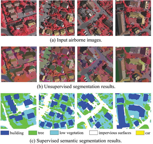
In Figure 2 we visually provide some segmentation results on the ISPRS airborne image datasets of Vaihingen (Gerke 2014). The unsupervised segmentation results are computed using Potts model (Storath et al. 2015), while the supervised segmentation results are predicted using PSPNet (Zhao et al. 2017). The unsupervised method tends to partition the image into piecewise segments with consistent gray values, while the supervised method aims to segment the image into semantically meaningful objects or classes with the help of the prior label information.

Figure 2. Examples of image segmentation of the ISPRS dataset (Gerke 2014).

3.2 Image matching

Image matching aims to find corresponding points between two or more images. It is the prerequisite for automated bundle adjustment and 3D reconstruction from multi-view images. For decades, image matching has attracted considerable attentions in both photogrammetry community (Gruen 2012) and computer vision community (Scharstein and Szeliski 2002).

Image matching can be divided into two categories: sparse matching and dense matching. Sparse matching aims to match corresponding points for bundle adjustment, image registration or applications that need well distributed corresponding points. As such, sparse matching algorithms only need to match key points with obvious appearance between images. Generally, image feature points are first extracted by using interest operators, such as Harris (Harris and Stephens 1988), Förstner (Förstner and Gülch 1987), DoG, SIFT (Lowe 2004), Daisy (Tola, Lepetit, and Fua 2010), or their variations. After that correspondences are established based on some matching algorithms that minimize certain similarity costs.

Different from sparse matching, dense matching is used for 3D reconstruction, which recovers the fine 3D structures of objects from multi-view images. In order to completely reconstruct the 3D shapes and textures of objects, matching is carried out as dense as possible. With the camera parameter $c$ being known, for two images $I_1\left(x,y\right)$ and $I_2\left(x,y\right)$, their epipolar images $I_{e1}\left(x,y\right)$ and $I_{e2}\left(x,y\right)$are generated. The general form of the dense matching problem is expressed as

(6) $\mathrm{m}\mathrm{i}\mathrm{n}E\left(M;I_1\left(x,y\right),I_2\left(x,y\right),c_1,c_2\right)$(6)

Currently, pixel-wise matchers are the mainstream dense matching methods. The problem of finding corresponding points between images is transformed to compute the pixel-wise disparity map between the left and right epipolar images. Specifically, the objective function of pixel-wise matching can be expressed as

(7) $E\left(M\right)={\sum }_p{\mathcal{D}}_m\left(p,M_p\right)+\lambda {\sum }_{q\in {\mathcal{N}}_p}{\mathcal{R}}_m\left(M_p,M_q\right)$(7)

where $p$ is a base image pixel in the left epipolar image $I_{e1}\left(x,y\right)$, $q$ is the pixel in the neighborhood ${\mathcal{N}}_p$ of $p$, $M_p$ and $M_q$ are disparity values of pixel $p$ and $q$, respectively. For a pixel $p={\left[x,y\right]}^{\mathrm{T}}$ with disparity of $M_p$, its corresponding pixel in the right epipolar image $I_{e2}\left(x,y\right)$, is $p^{\prime }={\left[x-M_p,y\right]}^{\mathrm{T}}$. The first term of Equation (7) is the sum of matching costs, while the second is the smoothness term used to constrain the continuity of the disparities of adjacent pixels, ${\mathcal{D}}_m\left(p,M_p\right)$ and ${\mathcal{R}}_m\left(M_p,M_q\right)$ are matching cost function and penalty function.

There are many kinds of matching cost functions. One of the simplest ones is the Sum of the Absolute Differences (SAD).

(8) $SAD={\sum }_p||I_{1p}-I_{2p^{\prime }}|{|}^2$(8)

where $I_{1p}$ is the pixel value of the pixel $p$ in the left image and $I_{2p^{\prime }}$ is the pixel value of its corresponding pixel in the right image. SAD assumes the lighting conditions of different images are constant, and the reflections with different zeniths and azimuths for the same location of the object are the same, which means that the reflectance function $f$ in Equations (1) and (2) is independent of the variables ${\theta }_i$, ${\phi }_i$, ${\theta }_r$ and ${\phi }_r$. This, in turn, means the corresponding points in different images have approximately equal pixel gray values. However, the actual situation is usually not ideal. The lighting conditions vary with time, and the reflections vary with zeniths and azimuths, reducing the effectiveness and robustness of SAD. More robust matching cost functions, such as Normalized Cross-Correlation (NCC) (Zhang and Gruen 2006), mutual information (MI) (Hirschmüller 2008), census (Zabih and Woodfill 1994), etc. are actually used.

The typical algorithms used to solve Equation (7) include Winner-Take-All (WTA), dynamic programming, scanline optimization, simulated annealing and graph cut (Scharstein and Szeliski 2002). Among them, WTA is a local solution that ignores the smoothness term, while the others are global solutions that consider the mutual constraints between matching results of adjacent pixels.

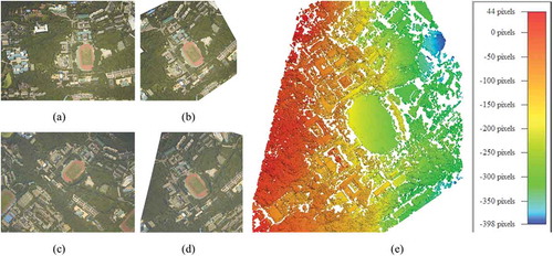
Figure 3 shows an example of dense matching of two aerial images of Wuhan University campus. Figure 3(a,c) is two input images $I_1\left(x,y\right)$ and $I_2\left(x,y\right)$, whose epipolar images $I_{e1}\left(x,y\right)$ and $I_{e2}\left(x,y\right)$ are Figure 3(b,d), respectively. Dense matching is performed using $I_{e1}\left(x,y\right)$ and $I_{e2}\left(x,y\right)$ as input, and the matching result is the pixel-wise disparity map of $I_{e1}\left(x,y\right)$, as shown in Figure 3(e), in which the disparity values are rendered by different colors.

Figure 3. An example of dense matching of two images of Wuhan University campus. (a) Left input image; (b) Left epipolar image; (c) Right input image; (d) Right epipolar image; (e) Matching result (disparity map) of the left epipolar image.

4. Object-image space tasks

4.1 Bundle adjustment

Bundle adjustment is an important step of Structure from Motion (SfM) (Zhang et al. 1999; Triggs et al. 1999). The classical SfM algorithm contains feature matching and bundle adjustment. Feature matching provides tie points between images for bundle adjustment, which simultaneously estimates the camera parameters and the corresponding object coordinates of the tie points through optimization.

Bundle adjustment is the procedure of refining a visual reconstruction to produce jointly optimal 3D structure and camera parameters (Triggs et al. 1999). It is based on the collinearity equations, i.e. the image point, object point and projection center all lying along a straight line which is the geometric process of the imaging. Theoretically, the image point of the same object point in different images should be the same. However, due to the noise in the image, image distortion and feature matching error, there is a difference between the measured image point and the projected image point from the estimated object point, i.e. the re-projection error. The re-projection equation is shown below:

(9) $\bar{x}=P\left(c,X\right)$(9)

where $\bar{x}=\left(x^{\prime },y^{\prime }\right)$ is the back-projected image point coordinates, $c$ is the camera parameters and $P$ is the projection function.

Considering a dataset with $m$ images and $n$ tie points generated by image matching, through minimizing the re-projection error, the 3D structure and camera parameters can be estimated.

(10) $minE\left(c,X;x,I\right)=\underset{\hspace{0.17em}}{{min}_{c_j,X_i}}{\sum }_{i=0}^n{\sum }_{j=0}^m||...||x_{i,j}-P{\left(c_j,X_i\right)}^2$(10)

where $X_i$ is the object coordinates of the $i$-th tie point, $c_j$ is the camera parameters of the $j$-th image, and $x_{i,j}$ is the image coordinates of $X_i$ in the $j$-th image.

Since the re-projection function is not linear, the bundle adjustment is a non-linear optimization process. The problem is complex because the number of parameters can be huge. Optimizing a large-scale non-linear function is not easy. Gradient Descent, Gauss-Newton and Levenberg-Marquardt or their variations are often used to solve the problem (Agarwal et al. 2010). These methods can achieve correct results when the initial guess of the camera parameters and 3D structure is good. However, a local optimal solution may be achieved under bad initial guess.

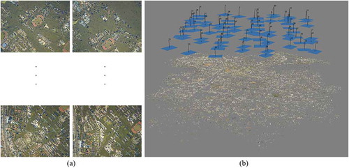
There are several products concerning bundle adjustment and SfM, such as VisualSFM (Wu 2016), COLMAP (Schonberger and Frahm 2016), Agisoft MetaShape (https://www.agisoft.com), etc. In this paper, a group of aerial images of Wuhan University campus are used as an example of bundle adjustment. As shown in Figure 4, MetaShape recovers the position and pointing of the camera and the 3D structure of the building successfully.

Figure 4. An example of bundle adjustment. (a) The input: original images and matched feature points; (b) The position and posture of the camera and the 3D structure of the building are recovered successfully using Agisoft MetaShape (https://www.agisoft.com).

4.2 SLAM

Simultaneous localization and mapping (SLAM) aims to build a map of the environment while simultaneously determining the location of a robot or a moving device. According to the sensors being used, SLAM can be categorized into three main types: laser-based, sonar-based and vision-based (i.e. image-based) (Aulinas et al. 2008). Considering that the vision-based SLAM (vSLAM) (Fuentes-Pacheco, Ruiz-Ascencio, and Rendón-Mancha 2015) is more popular, less expensive and more related to the imaging process, this paper is limited to this subject only. Essentially, the problems discussed by vSLAM and SfM are the same, i.e. estimating the camera parameters (called localization in vSLAM) and 3D structure (called mapping in vSLAM) from a sequence of images. Classical vSLAM system normally includes visual odometry, optimization, loop closing and mapping. The ultimate goal of vSLAM is real-time mapping and navigation. As such, all calculations, including route prediction, need to be done on-the-fly. In addition, as the images in vSLAM are collected incrementally, it is necessary to avoid or reduce the impact of drift, by Kalman filtering or optimization (Bresson et al. 2017). The mathematic details for vSLAM are similar to the ones of bundle adjustment as described in Section 4.1.

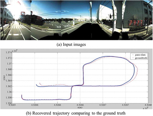
An example of vSLAM is shown in Figure 5 (Ji et al. 2020). The images were collected from a wide-baseline vehicle-mounted Ladybug camera which contains six fisheye lenses, five of which evenly cover a section of 360° horizontal scenes, and one fisheye lens points upward. Figure 5(a) shows the examples of the input fisheye images. The whole panoramic SLAM system is based on the fisheye calibration model, the panoramic model and the bundle adjustment (Ji et al. 2020), and several typical vSLAM steps, including initialization, tracking, key frame selection, local mapping, loop closure detection and global optimization (Mur-Artal and Tardos 2017). The recovered trajectory is shown in Figure 5(b) in comparison to the ground truth recorded with a highly accurate Applanix POS/AV navigation system (about 0.1 m localization accuracy).

Figure 5. An example of vSLAM from a multi-camera rig (Ji et al. 2020).

4.3 Shape from shading

Shape from shading aims to recover the shape from a single image or multiple images (Horn and Brooks 1986). From the imaging process, it is known that the image intensity is the interaction of illumination, surface albedo and surface normal. Since surface normal is the derivative of the surface shape, the shape can be recovered through solving the surface normal from the imaging model. Theoretically, it is a process of minimizing the difference between the image intensity and the inverse rendering. However, besides the surface normal, the illumination and surface albedo are usually unknown which makes the recovering of the surface normal from a single image an ill-posed problem. To make the problem solvable, the illumination and surface normal are often assumed to be known or constant (Zhang et al. 1999). Another kind of methods that relax the conditions in shape from shading is Photometric Stereo (PS) (Woodham 1980). It is demonstrated (Woodham 1980) that the surface normal can be recovered from multiple images captured from a fixed viewpoint under different illuminations. The problem is often solved with the variational method (Horn and Brooks 1986).

In recent years, shape from shading is also used to refine a surface known as a prior to a certain extent, especially combined with multi-view stereo (MVS) (Kim, Torii, and Okutomi 2016; Wu et al. 2011). MVS can be used to generate a coarse surface, which is then to be refined by shape from shading. For texture-less or texture-weak areas that are hard to handle by MVS, shape from shading can recover the fine shape. When refining using shape from shading, the coarse surface can provide an initial surface normal while the illumination and surface albedo can be estimated at first. The surface normal can then be further refined with proper constraint. The iteration of the two steps above makes the final surface shape well determined. The problem is often modeled as an energy function to be minimized through gradient descent or non-linear least squares method.

(11) $minE\left(\mathrm{\nabla }X,\rho ,L;c,I,X\right)=\underset{\mathrm{\nabla }X,\rho ,L}{min}{E}_{\mathrm{d}\mathrm{a}\mathrm{t}\mathrm{a}}\left(\mathrm{\nabla }X,\rho ,L\right)+\alpha E_{s1}\left(\mathrm{\nabla }X\right)+\beta E_{s2}\left(\rho \right)$(11)

where $\mathrm{\nabla }X$ is the vertex displacement along its normal, $\rho$ is the albedo of a vertex, $L$ is the illumination, $\alpha$ and $\beta$ are used to balance the data term $E_{\mathrm{d}\mathrm{a}\mathrm{t}\mathrm{a}}$, geometry smoothness term $E_{s1}$ and reflectance smoothness term $E_{s2}$. As shown above, shape from shading is also a reverse problem of the imaging process. When refining coarse surface, even the camera parameter $c$ is known and the illumination $L$, albedo $\rho$ in Equation (2) can be estimated with the coarse surface, there are still three unknown variables: the fine surface $X$, incident angle ${\theta }_i$, reflection angle ${\theta }_r$. As such, the Lambertian reflectance model which reflects equally in all directions is often assumed to eliminate the reflection angle ${\theta }_r$. As for the incident angle ${\theta }_i$, it can be estimated with the known imaging time and geographic coordinates for natural terrain. When dealing with other objects such as buildings, spherical harmonics (Basri and Jacobs 2001) are introduced, which use several variables and the surface normal to represent the imaging process for the scene.

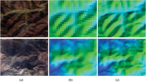
Based on the method of (Peng, Zhang, and Shan 2015) in which the 90 m SRTM is refined to 30 m with Landsat 8 imagery, the GaoFen-1 image is used to refine the SRTM from a resolution of 90 m to 15 m. The original resolution of GaoFen-1 image is 16 m and the resolution of SRTM is 90 m. At first, both the image and DEM are resampled to 15 m. Then, the shading-based DEM refinement algorithm is applied. At last, the DEM is refined to 15 m. As shown in Figure 6, the refined DEM is with higher resolution and with more geospatial details comparing to the original DEM.

Figure 6. An example of shape from shading for surface refinement. With (a) the GaoFen-1 image, the original SRTM is refined from a resolution of (b) 90 m to (c) 15 m using shape from shading.

5. Object space tasks

Tasks of or related to photogrammetry may also occur in object space, including point cloud registration (Besl and McKay 1992; Serafin and Grisetti 2015), point cloud segmentation (Golovinskiy and Funkhouser 2009; Papon et al. 2013), mesh generation (Shewchuk 2002) and object reconstruction (Yan, Shan, and Jiang 2014; Xiong et al. 2015), etc. The information such as point cloud in the tasks can be generated through Light Detection And Ranging (LiDAR) or stereo matching. Compared to LiDAR, the object information generated from stereo matching contains not only the geometric information but also the radiometric information in the images. Therefore, the information and method in the image space can also be considered for the object space tasks, e.g. considering the color information in point cloud segmentation and using shape from shading to refine the surface.

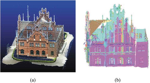
Among the tasks occurred in object space, a segmentation example of a point cloud derived from image matching is shown in Figure 7. It is worthwhile to note that point cloud segmentation is still an optimization problem and can be formulated with the optimization framework as following:

(12) $\mathrm{m}\mathrm{i}\mathrm{n}E\left(R;I,X\right)=\underset{\hspace{0.17em}}{{min}_R}\left({\sum }_{p\in P}{\mathcal{D}}_p\left(R_p\right)+\text{break}{\sum }_{p\in P}{\sum }_{q\in {\mathcal{N}}_p}{w}_{pq}\cdot \delta \left(R_p\ne R_q\right)+\text{break}{\sum }_{r\in \mathcal{L}}{h}_r\cdot \delta \left(r\in {\mathcal{L}}^{\prime }\right)\right)$(12)

where $P$ represents a set of data points whose coordinates are represented by $X$ in Equation (2), $R$ is the label of the points, ${\mathcal{N}}_p$ is an assumed neighborhood for the data point $p$, $\mathcal{L}$ is a given set of labels (e.g. planes), ${\mathcal{L}}^{\prime }$ is the set of labels appearing in $R$, ${\mathcal{D}}_p\left(.\right)$ is a function measuring the difference between data points and labels, $w_{pq}$ is the weight of the smooth term, $h_r$ is the weight of label and $\delta \left(.\right)$ is an indicator function. The first term is the data term which measures the discrepancy between data points and labels. The second term is the smooth term which measures the label inconsistency between neighboring points. The third term is the label term which measures the number of labels appearing in $R$.

Figure 7. A segmentation example of image matching derived point cloud (Nex et al. 2015): (a) point cloud generated by image matching (Schonberger and Frahm 2016; Schönberger et al. 2016), (b) optimized segmentation. Building point clouds are colored by segmented planar segments.

6. Concluding remarks

This paper expresses the imaging process under one physical and mathematical combined model. Photogrammetry is regarded as a reverse problem of the imaging process and formulated with one general optimization framework. Based on this unified framework, different tasks in photogrammetry are deducted to a special case of this framework. For each such task, we provide one representative solution and example. In summary, all the photogrammetry tasks are essentially the reversed imaging process and it can be formulated under one framework where different variables to be determined lead to different tasks.

It should be noted the division of tasks into image space, image-object space and object space reflects major domain that the problem is being solved. However, it does not mean no other space or information shall be involved at all. In fact, often times photogrammetric tasks are resolved in more than one domain if relevant and reliable information is available. It is not uncommon to see many solutions that work across multiple spaces but often with one being the major one.

Finally, we would like to restate the motivation of the work. The traditional theoretical framework for photogrammetry that has been used for decades could not fully reflect the current practices and meet the needs of a much broader community that are using photogrammetry techniques. This discipline certainly needs an imminent and necessary paradigm reshaping with rigorous and solid fundamentals. To this end, the paper presented a systematic and comprehensive structure with demonstrated examples for both research and learning.

Additional information

Notes on contributors

Jie Shan

Jie Shan is a Professor with the Lyles School of Civil Engineering, Purdue University, USA. His research interests include object extraction and reconstruction from images and point clouds, urban remote sensing, and data mining of spatial, temporal, and semantic data.

Zhihua Hu

Zhihua Hu is working toward PhD degree in photogrammetry and remote sensing. His current research interests include mesh refinement, and multi-view images 3D reconstruction.

Pengjie Tao

Pengjie Tao is currently an associate research fellow. His research interests include photogrammetry, registration of optical images and LiDAR points, and multi-view images 3D reconstruction.

Lei Wang

Lei Wang is working toward PhD degree in photogrammetry and remote sensing. His research interests include 3D computer vision, machine/deep learning, and 3D understanding.

Shenman Zhang

Shenman Zhang is pursuing toward PhD degree in photogrammetry and remote sensing. His current research interests include point clouds registration, and building reconstruction.

Shunping Ji

Shunping Ji is a Professor with the School of Remote Sensing and Information Engineering, Wuhan University. His research interests include photogrammetry, remote sensing image processing, mobile mapping system, and machine learning.

References

- Agarwal, S., N. Snavely, S. M. Seitz, and R. Szeliski. 2010. “Bundle Adjustment in the Large.” In European Conference on Computer Vision, September 5-11, 29–42. Hersonissos, Crete, Greece. doi:10.1007/978-3-642-15552-9_3.
- Aulinas, J., Y. Petillot, J. Salvi, and X. Lladó. 2008. “The SLAM Problem: A Survey.” In Frontiers in Artificial Intelligence and Applications 184 (1): 363–371. doi:10.3233/978-1-58603-925-7-363.
- Badrinarayanan, V., A. Kendall, and R. Cipolla. 2017. “SegNet: A Deep Convolutional Encoder-Decoder Architecture for Image Segmentation.” IEEE Transactions on Pattern Analysis and Machine Intelligence 39 (12): 2481–2495. doi:10.1109/TPAMI.2016.2644615.
- Bakker, W. H., L. L. F. Janssen, C. V. Reeves, B. G. H. Gorte, C. Pohl, M. J. C. Weir, J. A. Horn, A. Prakash, and T. Woldai. 2001. Principles of Remote Sensing - an Introductory Text Book. Enschede: ITC.
- Bar, L., T. F. Chan, G. Chung, M. Jung, N. Kiryati, N. Sochen, and L. A. Vese. 2015. “Mumford and Shah Model and Its Applications to Image Segmentation and Image Restoration.” In Handbook of Mathematical Methods in Imaging: Volume 1, 2 ed, 1095–1157. New York, NY: Springer. doi:10.1007/978-1-4939-0790-8_25.
- Basri, R., and D. Jacobs. 2001. “Lambertian Reflectances and Linear Subspaces.” IEEE International Conference on Computer Vision, July 9–12, 25, 383–390. Vancouver, Canada.
- Beardsley, P., P. Tort, and A. Zisserman. 1996. “3D Model Acquisition from Extended Image Sequences.” In European Conference on Computer Vision, April 14–18, 1065, 683–695. Cambridge, United Kingdom. doi:10.1007/3-540-61123-1_181.
- Besl, P. J., and N. D. McKay. 1992. “A Method for Registration of 3-D Shapes.” IEEE Transactions on Pattern Analysis and Machine Intelligence 1611: 586–606. doi:10.1109/34.121791.
- Boyd, S., and L. Vandenberghe. 2004. Convex Optimization. Cambridge, UK: Cambridge University Press. doi:10.1017/cbo9780511804441.
- Bresson, G., Z. Alsayed, L. Yu, and S. Glaser. 2017. “Simultaneous Localization and Mapping: A Survey of Current Trends in Autonomous Driving.” IEEE Transactions on Intelligent Vehicles 2 (3): 194–220. doi:10.1109/tiv.2017.2749181.
- Brown, M. Z., D. Burschka, and G. D. Hager. 2003. “Advances in Computational Stereo.” IEEE Transactions on Pattern Analysis and Machine Intelligence 25: 993–1008. doi:10.1109/TPAMI.2003.1217603.
- Chen, J., I. Dowman, S. Li, Z. Li, M. Madden, J. Mills, N. Paparoditis, et al. 2016. “Information from Imagery: ISPRS Scientific Vision and Research Agenda.” ISPRS Journal of Photogrammetry and Remote Sensing 115: 3–21. doi:10.1016/j.isprsjprs.2015.09.008.
- Chen, L. C., G. Papandreou, I. Kokkinos, K. Murphy, and A. L. Yuille. 2018. “DeepLab: Semantic Image Segmentation with Deep Convolutional Nets, Atrous Convolution, and Fully Connected CRFs.” IEEE Transactions on Pattern Analysis and Machine Intelligence 40 (4): 834–848. doi:10.1109/TPAMI.2017.2699184.
- Duchi, J., E. Hazan, and Y. Singer. 2011. “Adaptive Subgradient Methods for Online Learning and Stochastic Optimization.” Journal of Machine Learning Research 12: 2121–2159.
- Förstner, W., and E. Gülch. 1987. “A Fast Operator for Detection and Precise Location of Distinct Points, Corners and Centres of Circular Features.” In ISPRS Intercommission Workshop, June 2–4. Interlaken, Switzerland.
- Fuentes-Pacheco, J., J. Ruiz-Ascencio, and J. M. Rendón-Mancha. 2015. “Visual Simultaneous Localization and Mapping: A Survey.” Artificial Intelligence Review 43 (1): 55–81. doi:10.1007/s10462-012-9365-8.
- Furukawa, Y., and J. Ponce. 2009. “Accurate, Dense, and Robust Multiview Stereopsis.” IEEE Transactions on Pattern Analysis and Machine Intelligence 32 (8): 1362–1376. doi:10.1109/TPAMI.2009.161.
- Gerke, M. 2014. “Use of the Stair Vision Library within the ISPRS 2D Semantic Labeling Benchmark (Vaihingen).” Technical report. University of Twente.
- Golovinskiy, A., and T. Funkhouser. 2009. “Min-Cut Based Segmentation of Point Clouds.” In IEEE International Conference on Computer Vision Workshops, September 29-Octobor 2, 39–46. Kyoto, Japan. doi:10.1109/ICCVW.2009.5457721.
- Gruen, A. 2012. “Development and Status of Image Matching in Photogrammetry.” Photogrammetric Record 27 (137): 36–57. doi:10.1111/j.1477-9730.2011.00671.x.
- Gruen, A., and E. P. Baltsavias. 1987. “High-Precision Image Matching for Digital Terrain Model Generation.” Photogrammetria 42 (3): 97–112. doi:10.1016/0031-8663(87)90045-7.
- Harris, C. G., and M. Stephens. 1988. “A Combined Corner and Edge Detector.” In Procedings of the Alvey Vision Conference, August 31-September 2. Manchester, United Kindom. doi:10.5244/C.2.23.
- Hirschmüller, H. 2008. “Stereo Processing by Semiglobal Matching and Mutual Information.” IEEE Transactions on Pattern Analysis and Machine Intelligence 30 (2): 328–341. doi:10.1109/TPAMI.2007.1166.
- Horn, B. K. P. 1970. “Shape from Shading: A Method for Obtaining the Shape of A Smooth Opaque Object from One View.” Dissertation. Department of Electrical Engineering, The MIT Press.
- Horn, B. K. P., and M. J. Brooks. 1986. “The Variational Approach to Shape from Shading.” Computer Vision, Graphics and Image Processing 33 (2): 174–208. doi:10.1016/0734-189X(86)90114-3.
- Ji, S., Z. Qin, J. Shan, and M. Lu. 2020. “Panoramic SLAM from a Multiple Fisheye Camera Rig.” ISPRS Journal of Photogrammetry and Remote Sensing 159: 169–183. doi:10.1016/j.isprsjprs.2019.11.014.
- Kemelmacher-Shlizerman, I., and R. Basri. 2011. “3D Face Reconstruction from a Single Image Using a Single Reference Face Shape.” IEEE Transactions on Pattern Analysis and Machine Intelligence 33 (2): 394–405. doi:10.1109/TPAMI.2010.63.
- Kiefer, J., and J. Wolfowitz. 1952. “Stochastic Estimation of the Maximum of a Regression Function.” The Annals of Mathematical Statistics 23 (3): 462–466. doi:10.1214/aoms/1177729392.
- Kim, K., A. Torii, and M. Okutomi. 2016. “Multi-View Inverse Rendering under Arbitrary Illumination and Albedo.” In European Conference on Computer Vision, October 8–16, 750–767. Amsterdam, The Netherlands. doi:10.1007/978-3-319-46487-9_46.
- Kingma, D. P., and J. Ba. 2015. “Adam: A Method for Stochastic Gradient Descent.” International Conference on Learning Representations, May 7–9. San Diego, CA, USA.
- Klinker, G. J., S. A. Shafer, and T. Kanade. 1988. “Image Segmentation And Reflection Analysis Through Color.” In Applications of Artificial Intelligence VI 937: 229–244. doi:10.1117/12.946980.
- Li, D. 2000a. “Towards Photogrammetry and Remote Sensing: Status and Future Development.” Journal of Wuhan Technical University of Surveying and Mapping 2000: 1.
- Li, D., and J. Shan. 1989. “Quality Analysis of Bundle Block Adjustment with Navigation Data.” Photogrammetric Engineering & Remote Sensing 55: 1743–1746.
- Li, D., S. Wang, and Y. Zhou. 2008. An Introduction to Photogrammetry and Remote Sensing. 2nd Ed. Beijing: Publishing House of Surveying and Mapping.
- Li, D., Q. Zhu, and X. Li. 2000b. “Cybercity: Conception, Technical Supports and Typical Applications.” Geo-Spatial Information Science 3 (4): 1–8. doi:10.1007/BF02829388.
- Li, W., and Z. Fu. 2018. “Unmanned Aerial Vehicle Positioning Based on Multi-Sensor Information Fusion.” Geo-Spatial Information Science 21 (4): 302–310. doi:10.1080/10095020.2018.1465209.
- Lowe, D. G. 2004. “Distinctive Image Features from Scale-Invariant Keypoints.” International Journal of Computer Vision 60 (2): 91–110. doi:10.1023/B:VISI.0000029664.99615.94.
- Mumford, D., and J. Shah. 1989. “Optimal Approximations by Piecewise Smooth Functions and Associated Variational Problems.” Communications on Pure and Applied Mathematics 42 (5): 577–685. doi:10.1002/cpa.3160420503.
- Mur-Artal, R., and J. D. Tardos. 2017. “ORB-SLAM2: An Open-Source SLAM System for Monocular, Stereo, and RGB-D Cameras.” IEEE Transactions on Robotics 33 (5): 1255–1262. doi:10.1109/TRO.2017.2705103.
- Nex, F., M. Gerke, F. Remondino, H. J. Przybilla, M. Bäumker, and A. Zurhorst. 2015. “ISPRS Benchmark for Multi-Platform Photogrammetry.” ISPRS Annals of the Photogrammetry, Remote Sensing and Spatial Information Sciences II-3/W4: 135–142. doi:10.5194/isprsannals-II-3-W4-135-2015.
- Papon, J., A. Abramov, M. Schoeler, and F. Worgotter. 2013. “Voxel Cloud Connectivity Segmentation - Supervoxels for Point Clouds.” In IEEE Conference on Computer Vision and Pattern Recognition, June 23-27, 2027–2034. Oregon, Potland. doi:10.1109/CVPR.2013.264.
- Peng, J., Y. Zhang, and J. Shan. 2015. “Shading-Based DEM Refinement under a Comprehensive Imaging Model.” ISPRS Journal of Photogrammetry and Remote Sensing 110: 24–33. doi:10.1016/j.isprsjprs.2015.09.012.
- Real Ehrlich, C., and J. Blankenbach. 2019. “Indoor Localization for Pedestrians with Real-Time Capability Using Multi-Sensor Smartphones.” Geo-Spatial Information Science: 1–16. doi:10.1080/10095020.2019.1613778.
- Salah, M. B., A. Mitiche, and I. B. Ayed. 2010. “Multiregion Image Segmentation by Parametric Kernel Graph Cuts.” IEEE Transactions on Image Processing 20 (2): 545–557. doi:10.1109/TIP.2010.2066982.
- Scharstein, D., and R. Szeliski. 2002. “A Taxonomy and Evaluation of Dense Two-Frame Stereo Correspondence Algorithms.” International Journal of Computer Vision 47: 7–42. doi:10.1023/A:1014573219977.
- Schenk, T. 2005. Introduction to Photogrammetry. Columbus, OH: Department of Civil and Environmental Engineering and Geodetic Science, The Ohio State University.
- Schonberger, J. L., and J. M. Frahm. 2016. “Structure-from-Motion Revisited.” In IEEE Computer Society Conference on Computer Vision and Pattern Recognition, June 26-July 1, 4104–4113. Las Vegas, Nevada, USA. doi:10.1109/CVPR.2016.445.
- Schönberger, J. L., E. Zheng, J. M. Frahm, and M. Pollefeys. 2016. “Pixelwise View Selection for Unstructured Multi-View Stereo.” In European Conference on Computer Vision, October 8-16, 501–518. Amsterdam, The Netherlands. doi:10.1007/978-3-319-46487-9_31.
- Serafin, J., and G. Grisetti. 2015. “NICP: Dense Normal Based Point Cloud Registration.” In IEEE International Conference on Intelligent Robots and Systems, September 28-October 3, 742–749. Hamburg, Germany. doi:10.1109/IROS.2015.7353455.
- Shan, J. 2017. “Remote Sensing: From Trained Professionals to General Public.” Acta Geodaetica Et Cartographica Sinica 46 (10): 1434–1446. doi:doi.10.11947/j.AGCS.2017.20170361.
- Shan, J. 2018. “A Brief History and Essentials of Bundle Adjustment.” Geomatics and Information Science of Wuhan University 43 (12): 1797–1810. doi:10.13203/j.whugis20180331.
- Shelhamer, E., J. Long, and T. Darrell. 2017. “Fully Convolutional Networks for Semantic Segmentation.” IEEE Transactions on Pattern Analysis and Machine Intelligence 39 (4): 640–651. doi:10.1109/TPAMI.2016.2572683.
- Shewchuk, J. R. 2002. “Delaunay Refinement Algorithms for Triangular Mesh Generation.” Computational Geometry: Theory and Applications 22 (1–3): 21–74. doi:10.1016/S0925-7721(01)00047-5.
- Storath, M., A. Weinmann, J. Frikel, and M. Unser. 2015. “Joint Image Reconstruction and Segmentation Using the Potts Model.” Inverse Problems 31 (2): 025003. doi:10.1088/0266-5611/31/2/025003.
- Tola, E., V. Lepetit, and P. Fua. 2010. “DAISY: An Efficient Dense Descriptor Applied to Wide-Baseline Stereo.” IEEE Transactions on Pattern Analysis and Machine Intelligence 32 (5): 815–830. doi:10.1109/TPAMI.2009.77.
- Triggs, B., P. F. McLauchlan, R. I. Hartley, and A. W. Fitzgibbon. 1999. “Bundle Adjustment — A Modern Synthesis.” In International Workshop on Vision Algorithms, September 20-25, 298–372. Corfu, Greece. doi:10.1007/3-540-44480-7_21.
- Vu, N., and B. S. Manjunath. 2008. “Shape Prior Segmentation of Multiple Objects with Graph Cuts.” In IEEE Conference on Computer Vision and Pattern Recognition, June 23-28, 1–8. Anchorage, Alaska, USA. doi:10.1109/CVPR.2008.4587450.
- Wang, Z. 1990. Principle of Photogrammetry. Beijing: Publishing House of Surveying and Mapping.
- Woodham, R. J. 1980. “Photometric Method For Determining Surface Orientation From Multiple Images.” Optical Engineering 19 (1): 139–144. doi:10.1117/12.7972479.
- Wu, C. 2016. “VisualSFM : A Visual Structure from Motion System.” Accessed 11 January 2020. http://www.cs.washington.edu/homes/ccwu/vsfm
- Wu, C., B. Wilburn, Y. Matsushita, and C. Theobalt. 2011. “High-Quality Shape from Multi-View Stereo and Shading under General Illumination.” In IEEE Conference on Computer Vision and Pattern Recognition, June 20-25, 969–976. Colorado, USA. doi:10.1109/CVPR.2011.5995388.
- Xiong, B., M. Jancosek, S. Oude Elberink, and G. Vosselman. 2015. “Flexible Building Primitives for 3D Building Modeling.” ISPRS Journal of Photogrammetry and Remote Sensing 101: 275–290. doi:10.1016/j.isprsjprs.2015.01.002.
- Yan, J., J. Shan, and W. Jiang. 2014. “A Global Optimization Approach to Roof Segmentation from Airborne Lidar Point Clouds.” ISPRS Journal of Photogrammetry and Remote Sensing 94: 183–193. doi:10.1016/j.isprsjprs.2014.04.022.
- Yang, M., K. Yu, C. Zhang, Z. Li, and K. Yang. 2018. “DenseASPP for Semantic Segmentation in Street Scenes.” In IEEE Conference on Computer Vision and Pattern Recognition, June 18-22, 3684–3692. Salt Lake City, Utah, USA. doi:10.1109/CVPR.2018.00388.
- Zabih, R., and J. Woodfill. 1994. “Non-Parametric Local Transforms for Computing Visual Correspondence.” In European Conference on Computer Vision, May 2-6, 151–158. Stockholm, Sweden. doi:10.1007/bfb0028345.
- Zhang, H., J. E. Fritts, and S. A. Goldman. 2008. “Image Segmentation Evaluation: A Survey of Unsupervised Methods.” Computer Vision and Image Understanding 110 (2): 260–280. doi:10.1016/j.cviu.2007.08.003.
- Zhang, L., and A. Gruen. 2006. “Multi-Image Matching for DSM Generation from IKONOS Imagery.” ISPRS Journal of Photogrammetry and Remote Sensing 60 (3): 195–211. doi:10.1016/j.isprsjprs.2006.01.001.
- Zhang, R., P. S. Tsai, J. E. Cryer, and M. Shah. 1999. “Shape from Shading: A Survey.” IEEE Transactions on Pattern Analysis and Machine Intelligence 21 (8): 690–706. doi:10.1109/34.784284.
- Zhao, H., J. Shi, X. Qi, X. Wang, and J. Jia. 2017. “Pyramid Scene Parsing Network.” In IEEE Conference on Computer Vision and Pattern Recognition, July 21-26, 2881–2890. Honolulu, Hawaii, USA. doi: 10.1109/CVPR.2017.660.
- Zhao, W., L. Yan, and Y. Zhang. 2018. “Geometric-Constrained Multi-View Image Matching Method Based on Semi-Global Optimization.” Geo-Spatial Information Science 21 (2): 115–126. doi:10.1080/10095020.2018.1441754.