Support vector machine regression (SVR)-based nonlinear modeling of radiometric transforming relation for the coarse-resolution data-referenced relative radiometric normalization (RRN)

ABSTRACT

Radiometric normalization, as an essential step for multi-source and multi-temporal data processing, has received critical attention. Relative Radiometric Normalization (RRN) method has been primarily used for eliminating the radiometric inconsistency. The radiometric transforming relation between the subject image and the reference image is an essential aspect of RRN. Aimed at accurate radiometric transforming relation modeling, the learning-based non-linear regression method, Support Vector machine Regression (SVR) is used for fitting the complicated radiometric transforming relation for the coarse-resolution data-referenced RRN. To evaluate the effectiveness of the proposed method, a series of experiments are performed, including two synthetic data experiments and one real data experiment. And the proposed method is compared with other methods that use linear regression, Artificial Neural Network (ANN) or Random Forest (RF) for radiometric transforming relation modeling. The results show that the proposed method performs well on fitting the radiometric transforming relation and could enhance the RRN performance.

KEYWORDS:

• Support Vector machine Regression (SVR)
• non-linear
• radiometric transforming relation
• Relative Radiometric Normalization (RRN)
• multi-source data

1. Introduction

Remote sensing data have been widely applied in fields like agriculture, forest, environmental monitoring, etc. Integration of multi-source mid-resolution data plays a critical role in many fields, including regional and global scale research. However, the limitations of spatial and temporal resolution, revisit period, imaging conditions and other aspects can affect the availability of the useful data (Ban 2016; Navalgund, Jayaraman, and Roy 2007). However, due to some internal and external factors like sensor characteristics and atmospheric conditions and so on, radiometric inconsistency among multi-sensor or multi-temporal data (Beck et al. 2011) commonly exists, hindering the combination of multi-source remote sensing data. Therefore, radiometric normalization that can eliminate the radiometric inconsistency between multi-source data while preserving the real radiometric variation of the objects on Earth surface is a fundamental process, which can contribute to the efficient utilization of massive data (Tong 2016; Ujoh, Igbawua, and Paul 2019).

A variety of research conducted on the normalization of reflectance, temperature, vegetation, leaf area index and other data have been successfully applied in the fields of detailed mapping, regional climate response and urban dynamic monitoring (Masek et al. 2008). To eliminate the radiometric inconsistency among multi-source data, two main widely used methods are Absolute Radiometric Normalization (ARN) and Relative Radiometric Normalization (RRN). ARN corrects the effects of different factors separately, including atmospheric correction, terrain correction, angle correction, etc. And it is developed according to the remote sensing imaging process and the radiometric transferring process. In contrast, RRN builds the empirical radiometric transforming model and achieves the radiometric consistency through the relative radiometric transforming between the target image and the reference image (Yang and Lo 2000). And it is more applicable in some practical scenarios due to its low auxiliary data requirement.

Building the radiometric transforming model between the reference image and the subject image is the essence of RRN. And a large amount of models have been applied to this issue, for instance, the distribution-based models, such as histogram matching (Chavez and Mackinnon 1994), min-max normalization and mean-standard deviation normalization (Yuan and Elvidge 1996), use global image statistics to determine the adjustment on radiometric properties. And as to the pairwise pixel-based models, the generalized linear model is most widely used. Specifically, ordinary least square regression (Schott, Salvaggio, and Volchok 1988; Canty, Nielsen, and Schmidt 2004; Qaid et al. 2009), weighted linear regression (Zhang et al. 2008), hierarchical regression (Zhong, Xu, and Li 2015), Theil–Sen regression (Olthof et al. 2005), and orthogonal linear regression (Canty, Nielsen, and Schmidt 2004; Canty and Nielsen 2008) have been developed and used to correct the radiometric distortions.

However, the previous studies suggested the relations between observations of different sensors were non-linear models hard to be identified (Miura, Huete, and Yoshioka 2006). Linearity is not sufficient to accurately model cross-sensor radiometric transforming relation due to the complex light interactions, seasonality, local atmospheric conditions, illumination changes, and other possibly non-linear spectral transformations that unevenly affect the remote sensing images (Volpi, Camps-Valls, and Tuia 2015). And complex feature types make transformation relations more variable (Fan and Liu 2018). In our previous work, we demonstrated that the relation among different data is not a simple linear model but a spatial-heterogeneous and landscape variant model (Gan et al. 2014). Thus, the linear model will negatively affect the normalization results. Some recent researches toward the non-linearity have been proposed and performed well, such as the Artificial Neural Network (ANN)-based RRN (Sadeghi, Ahmaei, and Ebadi 2013) and the piecewise linear model-based RRN method (Sadeghi, Ahmaei, and Ebadi 2017), developed under the framework of the Pseudo-Invariant Features (PIFs)-based RRN. Meanwhile, some recently developed machine learning-based non-linear regression methods have achieved good performance in other fields. However, as to the coarse-resolution data-referenced RRN method which identifies the transforming relation based on the homogeneous pixels, few works have been carried toward the non-linearity of the transforming relation. It still remains an open issue to find an ideal model that can correctly transform all the images into a consistent status.

Therefore, we are motivated to improve the accuracy of RRN by inducing the Support Vector machine Regression (SVR) to identify the complex non-linear transformation between the subject image and the reference image. SVR is an algorithm developed based on the structural risk minimization statistical learning theory and is superior in the non-linear modeling. Although it was used in many fields and achieved good performance in the state of art methods, SVR has not been used for modeling the non-linear radiometric transforming relation. In this paper, we proposed an SVR-based RRN method under the coarse-resolution data-referenced RNN framework and explored the adaptability of SVR in the radiometric transforming relation modeling.

The remainder of this paper is organized as follows: Section 2 introduces the basic idea and specific implementation steps of the proposed method, as well as the parameter tuning method. In Section 3, three different synthetic data experiments are introduced, including data pre-processing. The experimental results are analyzed in Section 4. Finally, the conclusions are drawn in Section 5, discussing the pros and cons of the proposed method and future improvements.

2. Support vector machine regression-based relative radiometric normalization method

The proposed method, namely, supports vector machine regression-based relative radiometric normalization method (SVR-RRN) is developed under the framework of coarse-resolution data-referenced RRN (Gan et al. 2014), of which each fine-resolution subject data is related and adjusted to being radiometrically consistent with its corresponding coarse-resolution reference data. Different from the PIFs-based RRN approaches, which choose one of the multiple images as the reference image to normalize all the other images (i.e. subject image), the reference image is usually the synchronous coarser-resolution data of each subject image in our proposed method. Therefore, by inheriting the temporal and spatial radiometric consistency of the series of reference images, the consistency among the normalized subject images can be achieved.

Generally, the goal of RRN is to identify the radiometric transforming model between the subject image and the reference image. Let $S=\{S_1,S_2,S_3,\cdots \}$ be the subject image set and $R=\{R_1,R_2,R_3,\cdots \}$be the reference image set. The radiometric transforming model is identified to minimize the total difference between the reference image and subject image over the modeling sample set because the homogeneous pixels are usually less influenced by scale effect.

(1) $min\sum _{\hspace{0.17em}}dif(R_i,{S^{\prime }}_i)$(1)

where the normalized results $S_{\mathrm{i}}^{\prime }$ are generally expressed as:

(2) $S_i^{\prime }=f_i(S_i),i=1,2,\cdots ,n$(2)

where $f_i$ is the radiometric transforming model between the subject image $S_i$ and its corresponding reference image $R_i$, while $n$ is the total number of the imageries to be normalized. $f_i$ is generated through regression method by solving the optimization problem in Equation (1)(1) $min\sum _{\hspace{0.17em}}dif(R_i,{S^{\prime }}_i)$(1) . In our work, the SVR-RRN adopts the support vector machine regression to fit the radiometric transforming relation between the reference image and the subject image, i.e. the $f_i$ in Equation (2)(2) $S_i^{\prime }=f_i(S_i),i=1,2,\cdots ,n$(2) .

2.1. Support vector machine regression

Support vector machine has been developed by Cortes and Vapnik (1995), based on the structural risk minimization Statistical Learning Theory, and the Vapnik-Chervonenkis (VC) theory. In regression tasks, the SVR uses a cost function to measure the empirical risk in order to minimize the regression error. And the main algorithm basis of SVR is ε-insensitive function and Kernel function (Takeda, Farsiu, and Milanfar 2007), since the ε-insensitive loss function can disregard errors within a certain upper and lower range of the true value, thereby maintaining the sparseness and robustness of the fit. And the Kernel functions transform the data into a higher dimensional feature space to make it possible to perform the linear separation and improve the generalization ability, and finally obtain the non-linear learning algorithm in the original low-dimensional space.

In general, given the training sample set $(x_1,y_1),\cdots ,(x_i,y_i),x\in {\mathrm{R}}^{\mathrm{n}},\mathrm{y}\in \mathrm{R}$, the estimation function of linear relation in SVR takes the following form:

(3) $f(x)=\mathbf{w}\cdot \mathbf{x}+b$(3)

Now the question is to determine $w$ and $b$ from the training data by minimizing the regression risk based on the empirical risk:

(4) $R(w,\zeta ,{\zeta }^{\ast })=\frac{1}{2}{∥w∥}^2+C\sum _{i=1}^l({\zeta }_i+{\zeta }_i^{\ast })$(4)

where $C$ is a pre-specified value, and $\zeta ,{\zeta }^{\ast }$are slack variables used to measure the error of upside and downside, respectively.

Using the Lagrange function method to find the solution which minimizes the regression risk of Equation (3)(3) $f(x)=\mathbf{w}\cdot \mathbf{x}+b$(3) with the cost function in Equation (4)(4) $R(w,\zeta ,{\zeta }^{\ast })=\frac{1}{2}{∥w∥}^2+C\sum _{i=1}^l({\zeta }_i+{\zeta }_i^{\ast })$(4) , we obtain the following Quadratic Programming (QP) problem:

(5) $\underset{\alpha ,\alpha \ast }{max}{\mathrm{L}}_{\mathrm{D}}\left(\alpha ,\alpha \ast \right)=\underset{\alpha ,\alpha \ast }{max}\left\{\left.\begin{array}{c}-\frac{1}{2}\sum _{i,j=1}^l\left({\alpha }_i-{\alpha }_i^{\ast }\right)\left({\alpha }_j-{\alpha }_j^{\ast }\right)\left(x_i^{\mathbf{T}}\cdot x_j\right)\\ +\sum _{i=1}^l{\alpha }_i\left(y_i-\epsilon \right)-{\alpha }_i^{\ast }\left(y_i+\epsilon \right)\end{array}\right\}\right.$(5)

subject to:

$\begin{array}{rl}& 0\le {\alpha }_i\le C,i=1,\cdots ,l\\ & 0\le {\alpha }_i^{\ast }\le C,i=1,\cdots ,l\\ & \sum _{i,j=1}^l\left({\alpha }_i-{\alpha }_i^{\ast }\right)=0\end{array}$

We determine the Lagrange multipliers $\alpha$ and ${\alpha }^{\ast }$, then obtain:

(6) $\begin{array}{rl}& \bar{w}=\sum _{i=1}^l\left({\alpha }_i-{\alpha }_i^{\ast }\right)x_i\\ & \bar{b}=-\frac{1}{2}\bar{w}\left[x_r+x_s\right]\end{array}$(6)

When comes to the non-linear function, SVR uses Kernel functions to transform the data into a higher dimensional feature space, and corresponding QP problem is:

(7) $\underset{\alpha ,\alpha \ast }{max}{\mathrm{L}}_{\mathrm{D}}\left(\alpha ,\alpha \ast \right)=\underset{\alpha ,\alpha \ast }{max}\left\{\left.\begin{array}{c}\sum _{i=1}^l{\alpha }_i\left(y_i-\epsilon \right)-{\alpha }_i^{\ast }\left(y_i+\epsilon \right)\\ -\frac{1}{2}\sum _{i,j=1}^l\left({\alpha }_i-{\alpha }_i^{\ast }\right)\left({\alpha }_j-{\alpha }_j^{\ast }\right)\mathrm{K}\left(x_i,x_j\right)\end{array}\right\}\right.$(7)

The Kernel function $\mathrm{K}(x_i,x_j)$ is a symmetric function and satisfies the Mercer’s condition. After obtaining $\alpha$ and ${\alpha }^{\ast }$, we can get:

(8) $\bar{w}=\sum _{i=1}^l\left({\alpha }_i-{\alpha }_i^{\ast }\right)\mathrm{\Phi }(x_i)$(8)

Then, the estimation function becomes:

(9) $f(x)=\sum _{\mathrm{S}\mathrm{V}\mathrm{s}}\left({\bar{\alpha }}_i-{\bar{\alpha }}_i^{\ast }\right)K\left(x_i,x\right)+b$(9)

2.2. Workflow of the proposed SVR-RRN method

The main idea of the proposed method is to train the regression model using these aforementioned nonlinear regression methods and to obtain a global non-linear radiometric transforming model between the subject image and the coarse-resolution reference image. Then, the subject image is adjusted to be radiometrically consistent with the reference image. The specific process is shown in Figure 1.

Figure 1. Flowchart of the proposed SVR-RRN method.

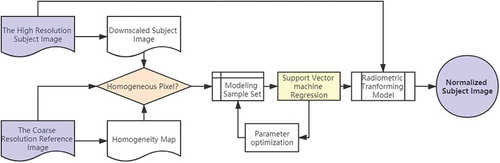
1. Pre-processing of images. One of the fine-resolution subject images is chosen to be the geolocation base, and all the coarse-resolution reference images and the rest subject images are co-registered to it.

2. Upscaling of the high-resolution subject image. The subject image S is resampled to the coarse-resolution unified with the reference image R, and the pixels pairs are formed to the candidate model sample set $\mathrm{\Omega }=\{(x_i,y_i),i=1,2,3,\cdots ,n\}$, where $x_i,y_i$ are the pixel value of point $i$ in subject image and reference image, respectively.

3. Selection of the homogeneous pixels. The heterogeneous pixels are excluded in the regression step due to the scale effect caused by the scale discrepancy between the subject image and the reference image. And the final sample set ${\mathrm{\Omega }}^{\prime }$ is obtained. Herein the homogeneity of each coarse pixel image is measured by purity (Gan et al. 2014).

4. Radiometric transforming model training. The model $f$ is trained by SVR based on homogeneous pixel set ${\mathrm{\Omega }}^{\prime }$ identified by Step 3. Herein, the common Radial Basis Function (RBF) and$\mathrm{K}\left(x_i,x\right)=exp\left(-\beta \cdot {∥x-x_i∥}^2\right)$ are utilized as the Kernel function. Meanwhile, the corresponding parameters are identified by the grid-search cross-validation (CV) method.

5. Radiometric transforming of the subject images. Based on the radiometric transforming model obtained in the previous step, pixel-by-pixel transforming is performed on the subject image with native spatial resolution to obtain the normalized result.

2.3. Parameter tuning

For SVR, parameter tuning is the key to obtain a valid model (Chapelle et al. 2002; Hsu, Chang, and Lin 2003). Both the parameters of the Kernel function and the setting of the error penalty factor have an essential impact on the performance of SVR. In our work, to balance fitting accuracy and model complexity, and to avoid overfitting, the CV method and the grid-search method are combined for parameter tuning (Browne 2000; Wang and Li 2005). Specifically, to optimize the parameters, we first gridded the potential values by a given optional data interval, then calculated the objective value at each grid point, and finally selected the optimal parameters corresponding to the optimal accuracy.

3. Experiments

In the aim of evaluating the effectiveness of the method, this paper takes the commonly used vegetation index NDVI as the experimental object and conducts some experiments to test the method to eliminate the radiometric inconsistency. The normalized result should be consistent with the reference data, nevertheless, with its native spatial resolution, it is hard to quantitatively evaluate in real application scenarios due to the lack of accuracy evaluation-reference data. Therefore, in this paper, two kinds of synthetic data experiments designed by Gan et al. (2014) are used to quantitatively assess the performance of SVR-RRN in eliminating the effects of different factors (Sections 3.1 and 3.2). Meanwhile, a real data experiment normalizing ASTER data and Landsat ETM+ SLC-off data is carried out, and the Landsat ETM+ SLC-off stripe region is filled by the normalized ASTER data. This is a case spatial complement of multiple data (Section 3.3). The detailed experiment scenarios design is shown in Table 1.

Table 1. Experiment scenarios design.

Experiment ID	Experiment	Factors involved in radiometric inconsistency
Experiment 1	Synthetic data	Atmospheric effect
Experiment 2–1	Synthetic data	Atmospheric effect, sensor character, viewing geometry
Experiment 2–2	Synthetic data	Atmospheric effect, sensor character, viewing geometry
Experiment 3	Real data	Atmospheric effect, sensor character, viewing geometry

The proposed method is compared with four other typical global methods, i.e. the linear model-based RRN (LSQ-RRN) and cluster-specified linear model-based RRN (CLM-RRN) (Martinez-Beltran et al. 2009; Zhu et al. 2010), the artificial neural network-based RRN (ANN-RRN) and random forest-based RRN (RF-RRN). The former two methods were formerly developed under the frame of the coarser-resolution data-referenced RRN method. And the latter two methods are developed here by introducing common learning-based nonlinear regression methods, i.e. ANN and RF, for radiometric transforming relation modeling under the coarser data-referenced RRN framework. Based on the consideration that ANN has been previously used in the nonlinear transforming relation fitting of reflectance data under the PIFs-based RRN framework (Sadeghi, Ahmaei, and Ebadi 2013), and RF regression was widely used for non-linear regression fitting in other fields (Breiman 2001). All the parameters involved in the regression procedure are tuned using the grid-search method introduced in Section 2.3 (as shown in Table 2).

Table 2. Parameters involved in the regression procedure.

Method	Parameter	Range
SVR-RRN	Penalty coefficient	[0.001, 0.01, 0.1, 1, 3, 5]
	Width of RBF Kernel	[0.003, 0.005, 0.01, 0.05]
ANN-RRN	Hidden layer number	[1, 2]
	Neuron numbers of 1st hidden layer	[5, 10, 15, 20]
	Neuron numbers of 2nd hidden layer	[5]
RF-RRN	Number of trees	[5,10, 20, 30]
	Minimum number of samples at a leaf node	[2, 3, 4]

Visual assessment and quantitative assessment are both performed to evaluate the accuracy. For quantitative assessment, each experiment is carried out 30 times based on a random subset of the original homogeneous pixel set. Subsequently, the mean value and standard deviation of the R² (coefficient of determination), RMSE (Root-Mean-Square Error), MAE (Mean Absolute Error) between the acquired normalized result and the evaluation-reference image are calculated. The results are considered to be more accurate when the MAE and RMSE values are smaller, and the R² values are larger.

3.1. Experiment 1 – eliminating the influence of atmosphere condition

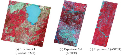
Synthetic data experiments are designed to evaluate the ability of eliminating radiative differences that are caused by the atmospheric effects. A medium-resolution data is atmospherically corrected and the Surface Reflectance (SR) is obtained at first. Secondly, the SR is upscaled to 250 m resolution and NDVI is calculated. Thirdly, the coarse-resolution NDVI is used as reference data to normalize the NDVI data that is calculated based on Digital Number (DN) at native resolution. Finally, the NDVI calculated based on SR is used as the evaluation-reference. Since the atmosphere effect is the only factor of inconsistency, thus, this synthetic data experiment is able to evaluate the performance of the normalization method in eliminating atmospheric effects, without being affected by other factors. Data used in this experiment are the Landsat-7 ETM+ data (WRS-2 path 114/29, acquired on 25 September 2011) located in the border between China and Russia, the Xingkai Lake and its surrounding area (as shown in Figure 2(a)). The representative land cover types include waterbody, farmland, forest and bare land. In addition, the Landsat Ecosystem Disturbance Adaptive Processing System (LEDAPS) is adopted to generate the SR data.

Figure 2. Study area of the experiments.

3.2. Experiment 2 – eliminating the influence of multiple factors

The method’s performance in eliminating the radiometric inconsistency caused by multiple factors (i.e. atmospheric effects and differences in sensor characteristics) is evaluated through two separate synthetic data experiments:

1. Experiment 2–1. This experiment is based on a pair of Synchronous mid-resolution data. One of the scene data is processed by atmospheric correction, and then upscaled to act as the coarse-resolution reference data for the other observation data. Meanwhile, the NDVI calculated from the SR of this data can be used as the evaluation-reference data. Because these two data are obtained on the same day, their NDVI should theoretically be equivalent. However, due to the effects of sensor characteristics, difference exists between the imaging geometry and atmospheric effects. This difference is expected to be eliminated after RRN. Therefore, this experiment can reflect the performance of RRN method in reducing the radiometric discrepancies caused by the above factors.

Data used in this experiment are a pair of synchronous Landsat ETM+ and Terra ASTER data acquired on 16 August 2000, near Hopkinsville, Kentucky, USA (as shown in Figure 2 (b)). The Landsat ETM+ data is atmospherically corrected using LEDAPS to generate the reference image. The ASTER NDVI based on DN is then normalized and evaluated by the Landsat ETM+ NDVI based on SR.

• (2) Experiment 2–2. In this experiment, a pair of coarse-resolution reference data and a fine-resolution subject image is utilized. Firstly, both of the coarse-resolution reference data and subject data are upscaled. Then, the upscaled reference data are used to normalize the upscaled subject data, and the original coarse-resolution data are used as the evaluation-reference data. In this experiment, the Landsat ETM+ data in Section 3.1 and its synchronous MODIS surface reflectance products are used as the subject data and reference data, respectively. The data are resampled to 250 m and 2 km, respectively. In this case, the radiometric inconsistency in this experiment scenario is contributable to the sensor differences, observed geometrical differences, and atmospheric influences.

3.3. Experiment 3 – experimenting on the real data

In this experiment, a pair of synchronous Landsat ETM+ and ASTER data on 21 May 2005 (Figure 2(c)) are obtained as the subject image. Their overlapping area covers the Portsmouth Harbor between Ohio and Virginia State, USA. The land cover consists of urban land, waterbodies, vegetation, bare soil, etc. Additionally, the synchronous MODIS surface reflectance products are used as the reference data. Both MODIS and ASTER data are geometric registered to ETM+. And ASTER data are spatially resampled to be consistent with ETM+ data. Using the proposed method, both the ASTER and ETM+ data are normalized separately, and the normalized ASTER data could be used to fill the stripe area of the Landsat ETM+ SLC-off image. The spatial complementarity between these two data is one of the typical scenarios for multi-source data integration. Meanwhile, contributed by the same image acquisition date and the overlapped non-striped regions, it is able to give a quantitative assessment of the consistency between the normalized results of these two data, therefore, quantitatively evaluate the performance of the proposed method on normalizing multi-source data.

4. Results and analysis

4.1. Performance in eliminating atmospheric effects caused inconsistency

Figure 3 shows the normalized results of Experiment 1. Visually, the normalized results have revealed greater changes than the data before normalization, exhibiting a spatial pattern and spatial distribution very similar to the evaluation-reference data. The scattergram (Figure 4) shows that the normalized result and the evaluation data yield good consistency.

Figure 3. Normalized results of Experiment 1.

Figure 4. Scattergram and distribution of difference between subject NDVI and evaluation-reference NDVI of Experiment 1.

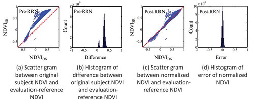
In this scenario, the radiometric inconsistency is solely caused by the atmospheric effects, and the average absolute error of the normalized results from the proposed method is 0.029 8, which indicates that most of the radiometric differences are eliminated than that before normalization (MAE: 0.263 5). It proves that the method proposed can effectively eliminate the differences between the data induced by the atmospheric effects.

Additionally, there is an obvious increase of the accuracy in our proposed method when compared with the linear model, LSQ-RRN. However, the proposed SVR-RRN has performed poorly than ANN-RRN and RF-RRN, while the CLM-RRN yields the highest accuracy (Table 3).

Table 3. Accuracy of normalization results in Experiment 1.

	Original	CLM-RRN	LSQ-RRN	ANN-RRN	RF-RRN	SVR-RRN
R^2	0.985 0	0.995 4 ± 0.000 0	0.985 1 ± 0.000 0	0.992 6 ± 0.000 0	0.991 2 ± 0.000 7	0.992 4 ± 0.000 7
RMSE	0.275 7	0.023 4 ± 0.000 0	0.043 2 ± 0.000 1	0.029 9 ± 0.000 1	0.033 0 ± 0.001 3	0.039 2 ± 0.003 5
MAE	0.263 5	0.015 1 ± 0.000 0	0.032 6 ± 0.000 2	0.021 0 ± 0.000 1	0.021 9 ± 0.000 6	0.029 8 ± 0.004 4

4.2. Performance in eliminating multiple factors caused inconsistency

4.2.1. Experiment 2–1: experiment based on a pair of synchronous fine-resolution data

The results of Experiment 2–1 are shown in Figure 5. Using the Downscaled ETM+ surface reflectance NDVI as reference data, the ASTER normalized result visually shows a larger change than pre-normalization. It exhibits a grayscale distribution similar to the evaluation-reference data (ETM+ surface reflectance NDVI at its native spatial resolution), and also the similar spatial pattern and spatial distribution.

Figure 5. Normalized results of Experiment 2–1.

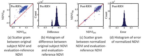
From the scattergram (Figure 6), the complex but obvious non-linear relation between subject data and reference data is well adjusted after normalization. The scattergram between the normalized result and the evaluation-reference data is distributed along the 1:1 line, and its MAE shifted from approximately 0.3 toward 0.03 (Table 4), which is greatly improved after normalization.

Figure 6. Scattergram and distribution of difference between subject NDVI and evaluation-reference NDVI of Experiment 2–1.

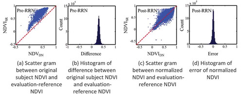
Table 4. Accuracy of normalization results in Experiment 2–1.

Indicator	Original	CLM-RRN	LSQ-RRN	ANN-RRN	RF-RRN	SVR-RRN
R^2	0.771 9	0.889 6 ± 0.000 1	0.857 2 ± 0.000 0	0.885 1 ± 0.000 6	0.866 3 ± 0.016 4	0.872 2 ± 0.008 1
RMSE	0.301 3	0.045 0 ± 0.000 0	0.053 8 ± 0.000 3	0.049 8 ± 0.000 9	0.049 3 ± 0.003 3	0.049 4 ± 0.002 2
MAE	0.294 5	0.027 9 ± 0.000 0	0.034 9 ± 0.000 3	0.035 6 ± 0.001 0	0.031 5 ± 0.002 0	0.030 1 ± 0.001 2

Table 4 shows that SVR-RRN still yields a good normalization effect in this experiment scenario. Specifically, the R² between the normalized results and the standard data has increased from 0.771 9 to 0.872 2, and the RMSE and MAE were reduced from 0.301 3 and 0.294 5 pre-normalization to 0.049 4 and 0.030 1 post, respectively.

Meanwhile, the proposed SVR-RRN method shows significant improvement to the LSQ-RRN, and performs slightly better than RF-RRN and ANN-RRN, but it is still not as good as CLM-RRN.

4.2.2. Experiment 2–2: experiment based on synchronous fine-resolution data and coarse-resolution data

The results of Experiment 2–2 are shown in Figure 7. The subject image has undergone significant visual changes and stays consistent with the evaluation-reference data after normalization. It is also strongly suggested from the scattergram and error distribution curve (Figure 8) that the normalization can effectively eliminate the radiometric inconsistency.

Figure 7. Normalized results of Experiment 2–2.

Figure 8. Scattergram and distribution of difference between subject NDVI and evaluation-reference NDVI of Experiment 2–2.

As can be seen from Table 5, the proposed method can effectively correct the impact induced by both the imaging environment and the sensor character. After normalization, MAE and RMSE dropped from 0.274 5 and 0.298 4 to 0.056 6 and 0.084 1, respectively. And in this scenario, SVR-RRN and RF-RRN perform similarly, better than LSQ-RRN and ANN-RRN, while worse than CLM-RRN.

Table 5. Accuracy of normalization results in Experiment 2–2.

Indicator	Original	CLM-RRN	LSQ-RRN	ANN-RRN	RF-RRN	SVR-RRN
R^2	0.909 0	0.953 8 ± 0.000 0	0.909 0 ± 0.000 0	0.932 0 ± 0.000 2	0.948 8 ± 0.000 2	0.948 3 ± 0.000 5
RMSE	0.298 4	0.079 3 ± 0.000 0	0.114 1 ± 0.000 0	0.097 2 ± 0.000 2	0.083 7 ± 0.000 2	0.084 1 ± 0.000 3
MAE	0.274 5	0.049 7 ± 0.000 0	0.083 8 ± 0.000 0	0.064 2 ± 0.000 2	0.053 4 ± 0.000 1	0.056 6 ± 0.000 6

4.3. Real data experiment

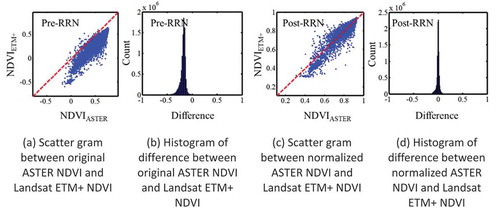
The Normalized ETM+ NDVI and ASTER NDVI are shown in Figure 9. And the scattergram and the error distribution curve (Figure 10) suggest that the complicated relation between the two prior to normalization is greatly corrected after normalization. The differences between them are also mostly eliminated. And the distribution of the difference between the normalized ASTER NDVI and ETM+ NDVI is almost normally distributed with mean equals to 0, which indicates that the proposed SVR-RRN method can effectively remove the differences between multi-source data and achieve good radiometric consistency between these two data by using the third-party coarse-resolution reference data as an intermediary.

Figure 9. Radiometric normalizing results of Experiment 3.

Figure 10. Scattergram and distribution of difference between ASTER NDVI and Landsat ETM+ NDVI of Experiment 3.

The overlapping non-striping areas from the resulted data are compared (Table 6). The difference between the NDVI data from different sensors was reduced to 0.0264 by the proposed method, and the average relative error has decreased from 0.196 3 to 0.041 3. Meanwhile, compared with the LSQ-RRN and CLM-RRN methods, the proposed method has the best R², MAE, RMSE accuracy. And the SVR-RRN yields a higher MAE than CLM-RRN but lower RMSE means that the CLM-RRN produces more high-biases than SVR-RRN. Besides, it should be noted that the RF-RRN performs even worse than the LSQ-RRN, which might be due to the random forests are prone to overfit to noises in regression tasks.

Table 6. Quantitative difference between ASTER NDVI and Landsat ETM+ NDVI in Experiment 3.

Indicator	Original	CLM-RRN	LSQ-RRN	ANN-RRN	RF-RRN	SVR-RRN
R^2	0.898 2	0.857 0 ± 0.000 5	0.898 2 ± 0.000 0	0.888 5 ± 0.001 2	0.782 8 ± 0.033 0	0.876 8 ± 0.031 1
RMSE	0.196 3	0.045 9 ± 0.000 1	0.043 5 ± 0.000 9	0.044 4 ± 0.000 7	0.060 6 ± 0.006 0	0.041 3 ± 0.006 2
MAE	0.187 5	0.026 0 ± 0.000 1	0.028 2 ± 0.000 6	0.028 9 ± 0.000 4	0.039 9 ± 0.004 4	0.026 4 ± 0.004 2

5. Conclusions and discussion

This paper proposes a support vector machine regression-based relative normalization method, which aims to model the complex non-linear radiometric relation among multi-sensor multi-temporal remote sensing data by taking advantage of SVR on solving non-linear problems. Based on multiple synthetic data experiments and one real data experiment, we analyze and evaluate the performance of SVR-RRN in different scenarios. The results show that this method can effectively eliminate the radiometric inconsistency caused by various factors, i.e. atmospheric effect, sensor differences and imaging geometry differences among the data, and reveal the value of SVR-RRN through real applications. Compared with other methods, contributed by SVR’s superiority in robustly fitting the non-linear model, the proposed method in this paper outperforms the LSQ-RRN and is robust in all experiment scenarios. And although in some scenarios, the proposed method is not as good as CLM-RRN, we should note that CLM-RRN relies on the land cover classification data (not always available) and easily leads to spatial non-continuous result. On the contrary, our proposed method has low auxiliary data requirements. Taking the above into consideration, we believe the SVR is better from the aspects of both implementation requirement and normalization accuracy, and the proposed method could effectively eliminate the radiometric inconsistency caused by various factors.

Since the model established in this method is a univariate regression model, only subject image and reference image are used for the model training. Therefore, the model is insufficient if used to perform special processing on some data points with abnormal patterns of radiometric inconsistency. The addition of other auxiliary information may be helpful for more accurate radiometric transforming. In future work, we will attempt in this regard to develop more accurate transforming models, precisely describing complex actual scenes, and procuring better relative radiometric normalization results.

Disclosure statement

No potential conflict of interest was reported by the author(s).

Additional information

Funding

This research was funded by the National Natural Science Fund of China [grant number 41701415] and Science fund project of Wuhan Institute of Technology [grant number K201724], Science and Technology Development Funds Project of Department of Transportation of Hubei Province [grant number 201900001].

Notes on contributors

Jing Geng

Jing Geng is a postdoctoral fellow in School of Computer Science and Technology, Beijing Institute of Technology. She received her Ph.D. degree in photogrammetry and remote sensing at Wuhan University. Her research interests include big data analysis and mining, and geospatial knowledge services.

Wenxia Gan

Wenxia Gan is an associate professor in School of Civil Engineering and Architecture, Wuhan Institute of Technology. She received her B.S., M.S. and Ph.D. degrees in Photogrammetry and Remote Sensing in Wuhan University, China, in 2009, 2011, 2015, respectively. Her research interests include radiometric calibration and rectification of remote sensing data, and application of RS/GIS on ecology environment.

Jinying Xu

Jinying Xu is a graduate student of Wuhan Institute of Technology. Her research interests include deep learning, and resource and environment monitoring with multi-sources satellite data.

Ruqin Yang

Ruqin Yang is an engineer in Wuhan Natural Resources and Planning Information Center. She received her Ph.D. degree in School of Resources and Environmental Sciences, Wuhan University. Her research interest is the application of multi-source data in the study of spatial planning and urban problems.

Shuliang Wang

Shuliang Wang is a professor of School of Computer Science and Technology, and the Executive Dean of Institute of E-Government, Beijing Institute of Technology in China. His research interests include spatial data mining and software engineering. For his innovatory study of spatial data mining, he was awarded the Fifth Annual InfoSciÒ-Journals Excellence in Research Awards of IGI Global, and one of the Best National Thesis in China. His authorized “Software and Applications of Spatial Data Mining” is one of the TOP TEN WIDM ARTICLES in 2016-2017.

References

- Ban, Y. 2016. “Multitemporal Remote Sensing: Methods and Applications.” Berlin Heidelberg: Springer-Verlag. doi:10.1007/978-3-319-47037-5.
- Beck, H. E., T. R. Mcvicar, A. I. J. M. V. Dijk, J. Schellekens, R. D. Jeu, and L. A. Bruijnzeel. 2011. “Global Evaluation of Four AVHRR–NDVI Data Sets: Intercomparison and Assessment against Landsat Imagery.” Remote Sensing of Environment 115 (10): 2547–2563. doi:10.1016/J.Rse.2011.05.012.
- Breiman, L. 2001. “Random Forests.” Machine Learning 45: 5–32. doi:10.1023/A:1010933404324.
- Browne, M. W. 2000. “Cross-Validation Methods.” Journal of Mathematical Psychology 44 (1): 108–132. doi:10.1006/Jmps.1999.1279.
- Canty, M. J., and A. A. Nielsen. 2008. “Automatic Radiometric Normalization of Multitemporal Satellite Imagery with the Iteratively Re-weighted MAD Transformation.” Remote Sensing of Environment 112 (3): 1025–1036. doi:10.1016/j.rse.2007.07.013.
- Canty, M. J., A. A. Nielsen, and M. Schmidt. 2004. “Automatic Radiometric Normalization of Multitemporal Satellite Imagery.” Remote Sensing of Environment 91 (3–4): 441–451. doi:10.1016/j.rse.2007.07.013.
- Chapelle, O., V. Vapnik, O. Bousquet, and S. Mukherjee. 2002. “Choosing Multiple Parameters for Support Vector Machines.” Machine Learning 46: 131–159. doi:10.1023/A:1012450327387.
- Chavez, P. S., and D. J. Mackinnon. 1994. “Automatic Detection of Vegetation Changes in the Southwestern United States Using Remotely Sensed Images.” Photogrammetric Engineering and Remote Sensing 60 (5): 571–583.
- Cortes, C., and V. N. Vapnik. 1995. “Support Vector Networks.” Machine Learning 20 (3): 273–297. doi:10.1023/A:1022627411411.
- Fan, F., and R. Liu. 2018. “Exploration of Spatial and Temporal Characteristics of PM2.5 Concentration in Guangzhou, China Using Wavelet Analysis and Modified Land Use Regression Model.” Geo-Spatial Information Science 21 (4): 311–321. doi:10.1080/10095020.2018.1523341.
- Gan, W., H. Shen, L. Zhang, and W. Gong. 2014. “Normalization of Medium-Resolution NDVI by the Use of Coarser Reference Data: Method and Evaluation.” International Journal of Remote Sensing 35 (21): 7400–7429. doi:10.1080/01431161.2014.968684.
- Hsu, C. W., C. C. Chang, and C. J. Lin. 2003. “A Practical Guide to Support Vector Classification.” Technical Report. http://www.csie.ntu.edu.tw/~cjlin/papers/guide/guide.pdf.
- Martinez-Beltran, C., M. A. O. Jochum, A. Calera, and J. Melia. 2009. “Multisensor Comparison of NDVI for a Semi-Arid Environment in Spain.” International Journal of Remote Sensing 30 (5–6): 1355–1384. doi:10.1080/01431160802509025.
- Masek, J. G., C. Huang, R. Wolfe, W. Cohen, F. Hall, and J. Kutler. 2008. “North American Forest Disturbance Mapped from a Decadal Landsat Record.” Remote Sensing of Environment 112 (6): 2914–2926. doi:10.1016/J.Rse.2008.02.010.
- Miura, T., A. Huete, and H. Yoshioka. 2006. “An Empirical Investigation of Cross-Sensor Relation S of Ndvi and Red/Near-Infrared Reflectance Using Eo-1 Hyperion Data.” Remote Sensing of Environment 100 (2): 223–236. doi:10.1016/J.Rse.2005.10.010.
- Navalgund, R. R., V. Jayaraman, and P. S. Roy. 2007. “Remote Sensing Applications: An Overview.” Current Science 93 (2): 1747–1766. doi:10.1073/Pnas.0710898105.
- Olthof, I., D. Pouliot, R. Fernandes, and R. Latifovic. 2005. “Landsat-7 ETM+ Radiometric Normalization Comparison for Northern Mapping Applications.” Remote Sensing of Environment 95 (3): 388–398. doi:10.1016/j.rse.2004.06.024.
- Qaid, A. M., H. T. Basavarajappa, S. Rajendran, S. A. Ashfaq, and J. Xu. 2009. “Calibration of ASTER and ETM+ Imagery Using Empirical Line Method—A Case Study of North-East of Hajjah, Yemen.” Geo-Spatial Information Science 12: 197–201. doi:10.1007/S11806-009-0052-0.
- Sadeghi, V., F. F. Ahmaei, and H. Ebadi. 2013. “A New Model for Automatic Normalization of Multitemporal Satellite Images Using Artificial Neural Network and Mathematical Methods.” Applied Mathematical Modelling 37 (9): 6437–6445. doi:10.1016/j.apm.2013.01.006.
- Sadeghi, V., F. F. Ahmaei, and H. Ebadi. 2017. “A New Automatic Regression-Based Approach for Relative Radiometric Normalization of Multitemporal Satellite Imagery.” Computational and Applied Mathematics 36: 825–842. doi:10.1007/s40314-015-0254-z.
- Schott, J. R., C. Salvaggio, and W. J. Volchok. 1988. “Radiometric Scene Normalization Using Pseudoinvariant Features.” Remote Sensing of Environment 26 (1): 15–16. doi:10.1016/0034-4257(88)90116-2.
- Takeda, H., S. Farsiu, and P. Milanfar. 2007. “Kernel Regression for Image Processing and Reconstruction.” IEEE Transactions on Image Process 16 (2): 349–366. doi:10.1109/TIP.2006.888330.
- Tong, X. D. 2016. “Progress in the Construction of China’s High-Resolution Earth Observation System.” Journal of Remote Sensing 20 (5): 775–780. doi:10.11834/Jrs.20166302.
- Ujoh, F., T. Igbawua, and M. O. Paul. 2019. “Suitability Mapping for Rice Cultivation in Benue State, Nigeria Using Satellite Data.” Geo-Spatial Information Science 22 (4): 332–344. doi:10.1080/10095020.2019.1637075.
- Volpi, M., G. Camps-Valls, and D. Tuia. 2015. “Spectral Alignment of Multi-Temporal Cross-Sensor Images with Automated Kernel Canonical Correlation Analysis.” ISPRS Journal of Photogrammetry and Remote Sensing 107: 50–63. doi:10.1016/j.isprsjprs.2015.02.005.
- Wang, X., and Z. Li. 2005. “Identifying the Parameters of the Kernel Function in Support Vector Machines Based on the Grid-Search Method.” Journal of Ocean University of China: Natural Science 35 (5): 859–862.
- Yang, X. J., and C. P. Lo. 2000. “Relative Radiometric Normalization Performance for Change Detection from Multi-Date Satellite Images.” Photogrammetric Engineering and Remote Sensing 66 (8): 967–980. doi:10.1080/01431160050030628.
- Yuan, D., and C. D. Elvidge. 1996. “Comparison of Relative Radiometric Normalization Techniques.” ISPRS Journal of Photogrammetry and Remote Sensing 51 (3): 117–126. doi:10.1016/0924-2716(96)00018-4.
- Zhang, L., L. Yang, H. Lin, and M. Liao. 2008. “Automatic Relative Radiometric Normalization Using Iteratively Weighted Least Square Regression.” International Journal of Remote Sensing 29 (2): 459–470. doi:10.1080/01431160701271990.
- Zhong, C., Q. Xu, and B. Li. 2015. “Relative Radiometric Normalization for Multitemporal Remote Sensing Images by Hierarchical Regression.” IEEE Geoscience and Remote Sensing Letters 13 (2): 217–221. doi:10.1109/LGRS.2015.2506643.
- Zhu, X., J. Chen, F. Gao, X. Chen, and J. G. Masek. 2010. “An Enhanced Spatial and Temporal Adaptive Reflectance Fusion Model for Complex Heterogeneous Regions.” Remote Sensing of Environment 114 (11): 2610–2623. doi:10.1016/J.Rse.2010.05.032.