Local color and morphological image feature based vegetation identification and its application to human environment street view vegetation mapping, or how green is our county?

ABSTRACT

Measuring the amount of vegetation in a given area on a large scale has long been accomplished using satellite and aerial imaging systems. These methods have been very reliable in measuring vegetation coverage accurately at the top of the canopy, but their capabilities are limited when it comes to identifying green vegetation located beneath the canopy cover. Measuring the amount of urban and suburban vegetation along a street network that is partially beneath the canopy has recently been introduced with the use of Google Street View (GSV) images, made accessible by the Google Street View Image API. Analyzing green vegetation through the use of GSV images can provide a comprehensive representation of the amount of green vegetation found within geographical regions of higher population density, and it facilitates an analysis performed at the street-level. In this paper we propose a fine-tuned color based image filtering and segmentation technique and we use it to define and map an urban green environment index. We deployed this image processing method and, using GSV images as a high-resolution GIS data source, we computed and mapped the green index of Milwaukee County, a 3,082 $k{m}^2$ urban/suburban county in Wisconsin. This approach generates a high-resolution street-level vegetation estimate that may prove valuable in urban planning and management, as well as for researchers investigating the correlation between environmental factors and human health outcomes.

KEYWORDS:

• Urban environment mapping
• greenview index
• panoramic street view
• urban landscape
• urban planning

1. Introduction

1.1. Background

Accurate quantification of vegetation biomass at different scales is a prominent and pressing issue for researchers in ecology and environmental science. In heavily forested areas, such as the Amazon rainforest, efficient tracking of vegetation in high volumes allows for monitoring large scale environmental phenomena such as deforestation. In urban environments, vegetation analysis can lend itself to applications in urban planning, and provide novel environmental data with which researchers can associate other known population health and socio-economic factors.

1.2. Imaging-based area vegetation estimation methods

High-volume vegetation analysis is commonly performed utilizing satellite and aerial imaging systems equipped with capabilities to detect light in the near-infrared (NIR) spectrum (Harbaš and Subašić 2014). Plant leaves possess strong reflectivity characteristics, reflecting a percentage of incoming near-infrared radiation in such a way that is relatively unique to vegetation making its identification feasible. Vegetation detection with NIR imaging connected to a satellite system is effective in capturing large areas in a few pictures from large distances, thus it is suitable for detecting forest canopy cover as well as grasslands and savannas. However, this method often fails to register vegetation located beneath natural or man-made canopy covers, so it is less reliable in identifying vegetation in urban environments.

In complex urban environments where the vegetation density gradient can change rapidly (on a meter scale) across regions, accurate aerial imaging can prove challenging. Not only can a highly variable man-made environment occasionally display NIR wave reflection similar to that of vegetation, but as vegetation density varies with large local gradients, the resolution of the imaging needs to change accordingly. In forested environments, lower resolution imaging suffices due to the high and relatively uniform density of vegetation. In urban environments, where vegetation can be quite sparse, higher resolution imaging is required. Additionally, for urban planning and other applications, more detailed vegetation data may be required for satisfactory analysis, and such data may be difficult to collect via satellite or aerial imaging. Proximity of the imaged data source to the image recorder may be necessary to accurately discern vegetation characteristics for a more detailed analysis.

An alternative approach to characterizing vegetation distribution could be based on the analysis of photographic images that are readily available for human environments. Google’s Google Street View (GSV) image data was designed to provide highly detailed local spatial information along the road system, and it is a readily available, economical and reasonably suitable data source for such a vegetation coverage analysis. Since its formation in 2007, the GSV-service has expanded significantly, with semi-regular visits to greater metropolitan and other densely populated areas for updates. Currently, GSV is providing high-resolution surround image data at the street-level on a massive, global scale.

In the middle of the past decade, researchers have begun utilizing methods to detect green vegetation within images on the street-level from the GSV database (Li et al. 2015; Richards and Edwards 2017). Using color-based image processing methods, a green vegetation index, or greenview index can be computed for a roadside surround image, and the obtained index value can be associated with the geographical position at which the image was taken. Such an index could be defined in a variety of ways, the most straightforward being the ratio of the pixels representing green vegetation within a street-level surround image and the total number of pixels contained in that image. Such a value is highly sensitive to the performance of the method that is used to identify green vegetation image pixels.

With the availability of a comprehensive, high-resolution and standardized quality street-level image database, this quantification method can be extended to a large-scale human-environment vegetation index. Defined along a road system, this human-environment vegetation index can then reflect green environments that the human population experiences in urban/suburban settings. Built on the GSV database that serves continuously updated fine resolution spatially annotated image information on the global scale and regular evaluation of such index would provide an objective, semi-current, quantitative representation of vegetation distribution. Furthermore, temporal changes in the natural urban-environment, from the human perspective, become documentable at an unprecedented scale and resolution.

In an early systematic approach to evaluate street-side vegetation, Li et al. (2015) provided a simple green color identification based unsupervised evaluation of street-side vegetation using GSV images. This method’s classification results are influenced by variance in illumination and are affected by misclassification of green non-vegetation image pixels. Improving this approach, Seiferling et al. (2017) applied a supervised geometric segmentation algorithm to identify vegetation pixels and measure vegetation cover in GSV images to classify image pixels into generic geometric classes such as ground plane, sky plane and vertical surfaces, without representing semantic image context. The approach requires pre-computation of image features and deficiencies in this process translate into misclassification of image pixels (Cai et al. 2018; Zhao et al. 2017). As an alternative, the supervised Pyramid Scene Parsing Network (PSPNet) algorithm was proposed by Zhou et al. (2019). PSPNet has improved on earlier pixel classification performance in urban environments (Cai et al. 2018; Zhao et al. 2017), when trained with data representing urban settings.

Stubbings, Rowe, and Arribas-Bel (2019) developed an approach based on Deep Convolutional Neural Networks (DCNN) and multilevel regression modeling to estimate a hierarchical area-level score of urban street-level trees, and semantic image segmentation was applied using the PSPNet (Zhao et al. 2017) to classify image pixels and estimate the percentage of vegetation cover in street-level images. Based on these individual image estimates, a hierarchical two-level modeling approach was used to derive an area score to correct for image-to-image variability due to the presence of “obstructing” urban features, account for sample variability, and incorporate measures of uncertainty.

In the following, we propose an image processing filtering method that dispenses with the labeled data requirements of supervised learning algorithms and avoids propagating deficiencies represented in training data. Instead, it returns to the primary problem of classifying vegetation image pixels and aims to correct mis-classification by incorporating a range of local characteristics of vegetation image pixels. Applied to surround GSV images, the output of the proposed image-filter provides a reliable quantification of greenness of the GSV measurement location as perceived by humans, however it does not attempt to identify the position of the in-view vegetation or non-vegetation components.

The proposed filtering method is extended to a processing pipeline that relies on data composed of diverse outdoors roadside images, compiled and distributed by the GSV service for data source, and it formulates a specific, computationally efficient image filtering work-flow for large scale analysis and mapping of urban vegetation. As shown in Figure 1, the Images were taken at a 5° pitch angle with camera heading rotation occurring in 60° increments. Rotation begins with the upper left image and moves across, down left, and across again. The result estimates a 360° panoramic view of the selected GSV location.

Figure 1. A sample Milwaukee GSV panoramic image series.

The presented workflow is designed to select and process high-volumes of publicly available GSV images and efficiently extract green vegetation pixels based on common local image characteristics. We will apply it to quantify and map both the street level surround view (for an instance of which see Figure 2) as well as that of the canopy cover of the urban forest in a Midwestern urban-suburban county, Milwaukee County, in the United States. The resulting mapping data is an estimate of greenness at the city-block resolution level, based on the block’s greenness in GSV images as it is viewed from its perimeter. Hence the resolution and the reliability of the estimate is expected to decrease with the size of city-blocks.

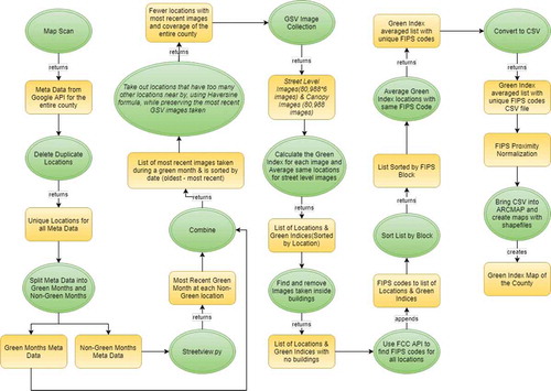
The results, visualized in Appendix A, and mapped in Section 4, offer a relatively high-resolution quantification for urban forest data with the potential to facilitate comparisons with other spatially distributed data, such as socio-economic or health data explored in Section 4.4. The main steps of the green vegetation extraction workflow are detailed in Sections 2–4, and a detailed view of the workflow is provided in Figure 2.

Figure 2. Green vegetation extraction workflow.

2. Identifying measurement locations

In this section we describe the data location selection stage of the green vegetation index mapping workflow. This stage consists of the steps preceding the GSV image collection effort as depicted in Figure 2.

2.1. Initial sweep of locations

Since 2007, Google’s GSV Service has accumulated a large database of surround images that constitute a high density coverage of much of the global road system. After registration, the general public has free, limited access to this database via the GSV API using GSV API keys. Gathering images from the GSV API requires a size specification for the requested image (width and height in pixels), a panorama image ID (PANO ID), a GSV API key, the camera heading specified in degrees, the field of view (FOV) in degrees, and the pitch of the camera in degrees. Querying GSV’s API for a specified PANO ID, with a longitude and latitude, heading, pitch, and field of view, the GSV API key returns a JPEG image according to the given specifications. Additionally, there is a meta-data service component available through the API that returns the location (latitude, longitude), the PANO ID, and the month of collection of the image closest to a requested latitude-longitude pair.

The first phase in our approach to identify and collect appropriate image data of the road system of Milwaukee County, was to query the GSV API database using the fast and unlimited access metadata query facility, through which we identify all viable image locations. In the first step, we covered Milwaukee County with a fine uniform grid of approximately 6 meter mesh size and collected the meta-data information for this grid. This was done to ensure complete coverage of all available GSV image locations along the county’s road system, to be further filtered. The mesh-size was determined experimentally to capture all positions with associated image data. From the 969 801 grid points interrogated for meta-data information (in June 2017), after discarding duplicates, we obtained over 200 000 unique GSV data points on the county’s road system along with the most recent image PANO IDs at these locations.

2.2. Filtering and sampling the initial sweep results

Since Milwaukee County lies in the North East Central Division of the United States, the local climate experiences high seasonal contrasts with a typically long and sub-freezing season extending from mid-late Fall into early-mid Spring. Local vegetation, that is dominantly green in the spring summer seasons (as seen on Figure 3(a)), can be expected to begin entering dormancy around the start of October and often beginning to bloom again near late April. The lack of presence of foliage or the inconsistency of its color during “non-green” months, as shown in Figure 3(b) and (c), limits reliable color-based identification of vegetation to image data from green months.

Figure 3. Milwaukee images during “green” and “non-green” months.

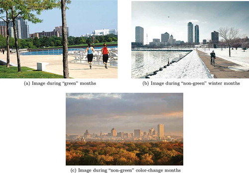
As a result of this extended period of dormancy, GSV images taken during these “non-green” months cannot reliably contain the information needed to properly quantify green vegetation densities. To maintain appropriate coverage of the area we focused on collecting green month images in place of the most recent images that were outside of our pre-determined May-September green month time period. A Python script was used to collect all historic GSV images that were taken at the collected locations (Letchford 2017). Provided with an image location, and with a specific associated PANO ID, the script returned all the GSV images historically taken at the specified location, along with the year and month date-stamp, and the associated panorama IDs. Using this script, we obtained an extensive historic list of panorama image data IDs that was accessible via the GSV API. Filtering these historical results to take only the most recent available green month data, we filled in 201 425 previously non-green locations as green locations utilizing the extended, historical GSV panoramic data. For the county, as of June 2017, most of the obtained data came from images captured in 2015 or 2011.

For each location we opted for collecting a panorama of images, specifically, six $640\times 640$ pixel images, each with a $90$° FOV taken in $60$° turns, resulting in a full $360$° surround capture of street-level view. Using all viable locations, the data collection would have required 1 824 628 image downloads, and with a GSV API limit of 25 000 free images per day per API Key, approximately 73 days to download all images. However, we observed that the obtained density of locations was extremely high, with many locations falling within just a meter of one another along a roadway. Given that GSV images can often provide well over a 10 meter range of quality view along the road and into the roadside, this density of images is unnecessary.

In a need to reduce the data collection load, as well as the computational load for the subsequent image analysis task, a data location filter thinning algorithm was designed and performed to obtain a lower and uniform density road system coverage, composed of most recent green month image data. The thinning was performed in a single pass on descending time ordered data by sequentially and dynamically updating the data set. At each step, we eliminated all data points except for the $n$ most recent ones that are pursuant to (i.e., older than) the data point in focus and that are located within a circle of radius $R$ (meters) centered at the data point in focus. In our case, application of the thinning algorithm with the parameter choices of $n=2$ and $R=6$ produced the desired data-reduction, down to 80 985 well-distributed green month data points, mostly dated 2011 or later.

For this dataset, the new maximum download time at a 6 images per location rate (for a total of 485 910 images) using a single GSV API key was approximately 20 days. In a team effort, using multiple keys the actual image download time was under 8 days with an average download speed of 20–50 mbps.

3. Image segmentation

To segment our outdoors images into vegetation and non-vegetation image components we employed a highly computationally efficient multi-filter image segmentation algorithm that was formulated based on a set of heuristics motivated by studying the color characteristics of collected GSV data.The steps of segmenting images and determining vegetation/non-vegetation pixels are summarized in Figure 4.

Figure 4. Vegetation extraction image processing flow chart.

3.1. Color spaces and heuristics

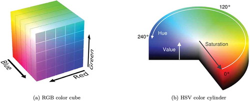
Considering typical characteristics that could generally differentiate vegetation component pixels on photographic images, we identified pixel color and the local variation of color in a neighborhood of the image pixel. Specifically, we focused on identifying and exploiting these characteristics on the GSV images. Working with pixel color information, we rely on two separate color representation standards: the RGB and the HSV color spaces (see Figure 5). The GSV data we collect uses the RGB color representation. The RGB standard represents pixel colors with values in the unit cube of ${\mathbb{R}}^3$ in Cartesian coordinates (interpreted as an additive weighted mixture of the primary colors Red, Green, and Blue) or in many implementations simply as a quantized mesh of the scaled unit cube, typically with values ranging from 0 to 255 in each color channel (Figure 5(a)). The HSV (i.e. Hue-Saturation-Value) color space represents color in the closed unit cylinder in cylindrical coordinates (Figure 5(b)), with Hue and Saturation being the polar coordinate components, and the cylindrical component Value is related to light intensity.

Figure 5. RGB and HSV color space representations.

A standard condition for identifying green pixel colors in RGB representation is given by the formula $2G>R+B$. This simple condition is used e.g., in Li et al. (2015), which in its calculations relies on the assumption that the presence of generic green color in an outdoors image corresponds to vegetation.

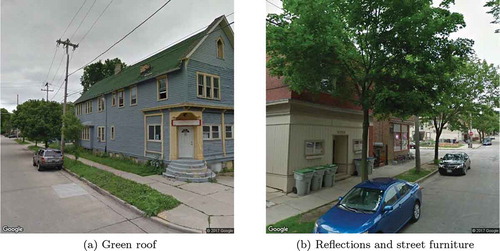
While shades of green vary in images with different types of vegetation, as well as within single units of a given type, most vegetation displays a substantial green color component within certain frequency ranges. However, exploiting this commonality to identify vegetation in a complex image is a nontrivial task, and while it is easy to identify pixel colors that are dominated by a green color component, the task also involves differentiating green pixels of vegetation from similarly colored “artificial green” image pixels. Artificial green colored artifacts in an outdoors image may include, but are not limited to, green painted structures (houses, bridges, buildings, street furniture etc.), green-colored vehicles, reflections of vegetation on smooth surfaces, and clothing of pedestrians within the image frame. In particular, Milwaukee County is home to green road and street signs, green garbage cans, dumpsters, and buses, all of which repeatedly appear in GSV images and in some cases could form a sizable component within them.

Common non-vegetation or “artificial green” structures or other objects of various sizes commonly occur in GSV images and can lead to false detection. Such artificial objects include green roof tops, as shown in Figure 6(a), green-colored street furniture such as trashcans, reflections of vegetation in the car windows as shown in Figure 6(b), or street and traffic signs.

Figure 6. Non-vegetation green street view image components.

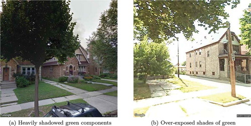
Google makes an effort to ensure proper lighting conditions: that all GSV images are captured in daylight under adequate weather conditions to minimize image quality inconsistencies between locations. The result of this is that time of day and sub-optimal light conditions are less likely to influence the GSV images. However, Google’s image collection standards are not able to fully control lighting variations in the collected daytime images. Cloud coverage, the sun’s position in the sky and shadowing can all substantially affect lighting variation between locations or within a single image frame. In street-view images, as shown in Figure 7, heavily shadowed areas may become near black or the color of highly overexposed areas shift toward white. In particular, trees with large canopies often exhibit heavy shadowing effects depending on the sun’s position, as seen in Figure 7(a), where it can be observed how the tree canopy in the foreground is heavily shadowed due to environmental lighting. Suburban grass and shrubs exposed to a high intensity light in differential shading conditions can become overexposed and near white in appearance, as in Figure 7(b), where GSV image on the left is highly overexposed, with vegetation giving off yellow coloring and grass becoming nearly indistinguishable from the pavement. Due to the structure of the RGB color space, it becomes difficult to identify vegetation in images with largely varying lighting scenarios relying on RGB-based color filters.

Figure 7. Extreme GSV lighting scenarios.

Additionally, a common property of human-created artificial green structures is their relative local color consistency and low color variation. For instance, at least locally, a painted structure or a car is mostly colored with a single shade of green, exhibiting only small and smooth variations from a primary, dominating color shade. Natural vegetation on the other hand rarely has such color features, often exhibiting large variational changes in green, reflecting more complex geometry and structure.

3.2. Segmentation algorithm

We utilize the observations and heuristics outlined above to formulate a multi-component vegetation image-segmenter, that avoids chronic errors induced by the presence of artificial green colored objects and improper lighting.

In an initial step of the segmentation algorithm, performed in HSV representation, we saturate the images by scaling the S color component by a factor $\kappa >1$. This is done to compensate for shading variation before the additional filtering steps.

After the pixel color saturation step, to segment the images we apply and combine the results of a series of three independent logical-valued image filters or masks, parameterized by the values $(\alpha ,\beta ,\gamma )=(1.5,0.4174,\text{break}0.1569)$ and localization parameter $m=5$:

1. in the original RGB color space with the parameterized condition $2G>\alpha (R+B),$ we select a restricted subset of the generic green image pixels;

2. with the hue-limiting condition $H<\beta$, we additionally exclude image pixels with a substantial blue component that is characteristic of many “artificial” green pixel colors; and

3. using all three RGB channels, we apply a binary filter composed from local rank filters to exclude image locations with neighborhoods of low local variations, specifically selecting pixels that satisfy the condition

   $min(R_{max}-R_{min},G_{max}-G_{min},B_{max}-B_{min})>\gamma .$

   Here $X_{max}$ and $X_{min}$ are the maximal and minimal rank filters in a local neighborhood of pixels size $m$, centered at the pixel location, with $X\in \left\{R,G,B\right\}$.

The parameter values $\kappa ,\alpha ,\beta ,\gamma$ and the shape and size $m$ of the local neighborhood used in our implementation were determined based on the segmentation performance on a representative test set of several hundred images that were hand-selected and evaluated to include a wide variety of image features occurring in GSV images. Figure 8 illustrates the dependence of segmentation on parameter values in the first image filter. In a “Liberal Cut” (Figure 8(b)), we have false positive errors induced by the use of a wide pass-band color processing filter. Almost all vegetation within the original image is present, at the expense of inclusion of some building structure pixels remaining from the non-green background post-processing. In a “Conservative Cut” (Figure 8(c)), we have an over-processed image resulting from too restrictive of a color-processing method. No artificial green pixel is present, albeit at the loss of more substantial false negative vegetation pixel data.

Figure 8. Errors induced by under- and over-processing vegetation filter parametrizations.

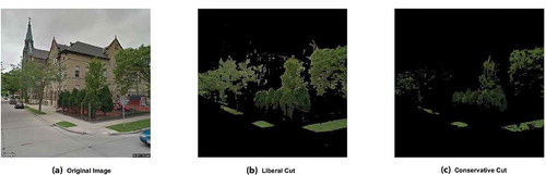
Figure 9. Artificial green image component removal.

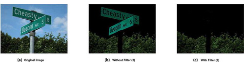
Figure 9 examplifies how the second image filter component improves performance by identifying and removing artificial green hue-values commonly found in man-made objects such as recurring street and road signs as well as buildings and street furniture.

3.3. Index calculation

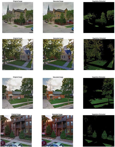
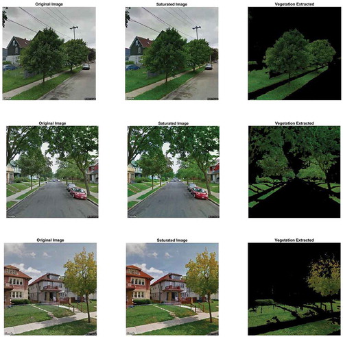
In performing the segmentation algorithm discussed above, pixels deemed as being non-vegetation had their RGB values altered to $(0,0,0)$, or black, with the remaining pixels (deemed as vegetation pixels) left unaltered. See Appendix A for several examples.

After analyzing each of the 409 600 pixels within an image, a green index for that image was calculated as:

$\mathrm{G}\mathrm{r}\mathrm{e}\mathrm{e}\mathrm{n}\mathrm{I}\mathrm{n}\mathrm{d}\mathrm{e}\mathrm{x}=\frac{\mathrm{v}\mathrm{e}\mathrm{g}\mathrm{e}\mathrm{t}\mathrm{a}\mathrm{t}\mathrm{i}\mathrm{o}\mathrm{n}\mathrm{p}\mathrm{i}\mathrm{x}\mathrm{e}\mathrm{l}\mathrm{s}}{\mathrm{t}\mathrm{o}\mathrm{t}\mathrm{a}\mathrm{l}\mathrm{p}\mathrm{i}\mathrm{x}\mathrm{e}\mathrm{l}\mathrm{s}}\times 100\mathrm{\%}$

giving us a resulting percentage of vegetation visible within the image frame. Performing this analysis for each of the six images forming the panoramic set, and averaging the result, we are left with a percentage value of visible green vegetation found at that location. Computational time for the entire image processing structure presented in Figure 4 varied between 0.1–0.2 seconds/image, running on an Intel quad-core i7-4702HQ CPU.

4. City-block level mapping with proximity normalization

After evaluating the street-level green index values for the 80 985 green month GSV locations covering the road system of Milwaukee County, the ArcMap component of Esri’s ArcGIS software was used to visualize the county’s fine resolution green index data as a color coded map of urban vegetation information.

4.1. Initial mapping

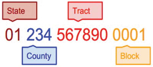
The county’s green index distribution can be mapped at the Federal Information Processing Standard (FIPS) tabulation track or block level resolutions, that are identified using standardized maps associated with the FIPS codes. For the structure of FIPS codes see Figure 10. For each location coded by the GSV latitude-longitude data values, the position was mapped to a Federal Information Processing Standard (FIPS) code and the obtained index values were averaged at the FIPS block-level; obtaining an index value for each city-block represented in an FIPS block-level shapefile. The FIPS code conversion was verified using the Federal Communications Commission’s (FCC) census block conversions API. The green-index value range was represented in a linear color scale ranging between dark brown and light green.

Figure 10. Sample FIPS code.

The result of this initial procedure is a color-ramped map which can be seen on Figure 12(a). Through examination of this map, it becomes readily apparent that quantities of data for particular city-blocks are missing. In fact, a total of 1 199 individual blocks lack any sort of viable green index data. Furthermore, upon closer inspection, it becomes apparent that the number of unique GSV locations utilized in the mean green index calculation for each FIPS city-block vary highly between neighboring blocks (Figure 11). The values inside each city-block denote the number of GSV locations used to calculate that block’s average green index. Note the discrepancies between adjacent blocks contained within the red regions. Some city-blocks use up to twelve unique GSV locations to create their mean green index, while neighboring blocks use as few as three unique GSV locations. In extreme cases, some blocks (in yellow) received no GSV vegetation data, while neighboring blocks in close proximity had several.

The source of this error is due to the fact that, in this procedure, although most measurement locations a on or near the border of two or more FIPS blocks, each obtained GSV location index is assigned to only one FIPS block (in which its true GSV latitudinal-longitudinal position appears). As an example, in this prior procedure, if a GSV vehicle were driving along the east side of a road, the index data computed at the vehicle’s exact latitudinal-longitudinal position would be mapped into the nearest geographic FIPS block, in this case on the east side of the road. However, given that we are utilizing panoramic imaging data, it follows that the same image component information should apply to all geographic FIPS blocks within a small radius centered around the exact GSV measurement location.

Figure 11. Initial mapping errors.

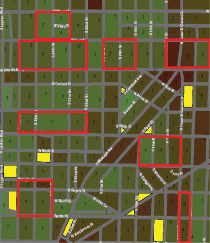
Figure 12. Milwaukee County raw green index FIPS block map, and its correction by proximity normalization.

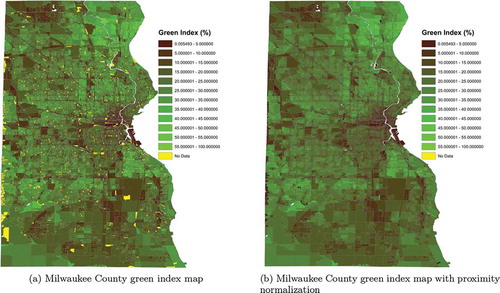
4.2. Proximity normalization

To rectify the FIPS mapping issues discussed in Section 4.1, we performed an alternative index assignment algorithm which we termed proximity normalization. This normalization method takes the green index value computed from the street-level surround imaging of a chosen GSV location and, before averaging, assigns the index value to (possibly multiple) FIPS-blocks in the vicinity of the GSV location. Specifically, a GSV location may be assigned to as many as 6 different city-blocks containing the same geographic information within a 5-meter radius of the GSV origin. This is done through segmentation of the 5-meter radius circle around the GSV location into 6 unique headings: true north, $60$° to the east and west of true north, $120$° to the east and west of true north, and true south.

Because our data relies on FIPS codes associated to latitude-longitude values, the Great Circle Distance Haversine Formula was employed in measuring the circle radius around the chosen GSV location. The index value associated with the selected GSV location was then assigned for averaging to each of the unique FIPS codes containing at least one of the surrounding positions. This smoothing procedure eliminates the FIPS block codes with missing and sparse information, and generally produces high-quality index maps at the city-block resolution. Through this process, we are given a better reflection of the vegetation content within Milwaukee County, without increasing the number of analyzed points. For visualization results, see Figure 12(b). We note that both maps on Figure 12 possess identical color legends, with all 1 199 “no data” city-blocks having been successfully corrected post-normalization.

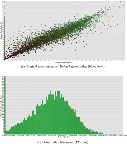
The changes effected by the proximity normalization method are illustrated on Figure 13(a), where each city-block’s horizontal axis coordinate is the block’s original green index value, and its vertical axis coordinate is given by the post-normalization index value. Green index color annotation is as defined on Figure 12. The resulting County green index distribution with a 120 bin histogram is shown on Figure 13(b). Note the high-quantity of $0\mathrm{\%}$ indices; these locations are most commonly found in areas within downtown Milwaukee. Computing an average green index value for Milwaukee County as a whole gives us a mean value of $23.55\mathrm{\%}$.

Figure 13. The impact of proximity normalization on the green index assignment.

4.3. Further mapping

Upon completion of the proximity normalization step, a resulting high-resolution map can be created not only at the city-block level, but at the street-level as well. Utilizing ArcMap’s geographic coordinate system conversion toolbox, latitudinal-longitudinal data for each panoramic GSV street car location was projected onto a Milwaukee County shapefile containing road network data. Placing a small diameter circle on each GSV street car location utilized in our vegetation calculations, and color coding each circle using the same index color legend as at the city-block level, we can create a vegetation map at the individual latitude-longitude coordinate level. Through this process, a resulting representation of visible vegetation is displayed at individual locations, accurate to within just a few meters. See Figure 14 for a sample area visualization.

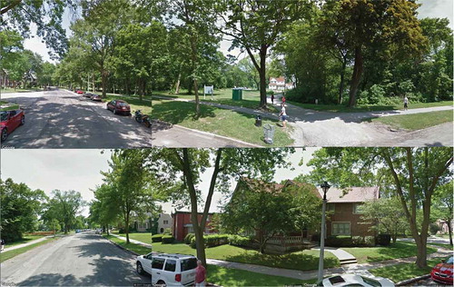
Figure 14. Milwaukee county vegetation maps in more detail.

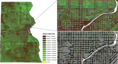
Both images on the right of Figure 14 display the same location along the Milwaukee River, with the map on the left highlighting the area in a red-bordered rectangle located in East-Milwaukee. The upper-right map color codes each city-block with its respective mean index value, while the lower-right map uses the same color coding at the individual latitudinal-longitudinal geographic (street-level) positions. The numbers located within each city-block correspond to the number of GSV locations that contributed to that block’s average index computation.

For an interactive visualization of the high-resolution GSV mapping developed here, we encourage the reader to visit the website https://mke-green-index.netlify.com/, where the entire Milwaukee county street-level Green-index map can be explored both at the FIPS track and block levels, and at the level of individual imaging positions. Additionally, all individual street-view surround image-composites that were used to evaluate the index can be viewed, along with the segmentation algorithm’s results on these image-composites (Honts 2020).

4.4. Data comparison capabilities

From the processes presented in Sections 2, 3, 4.1, 4.2, and 4.3, we are left with high-resolution vegetation data at both the street and city-block levels. Repeating the processes of Sections 4.1 and 4.2 using alternate lower-resolution FIPS groups, we can adjust the averaging indices of our data such that alternate maps can be created with large FIPS groupings. Due to the fact that much of the publicly available city and county-wide data for health and socio-economics is gathered using either city-block, block-group, tract-level, ZIP code-level, city-level, or county-level resolution groups, the benefit of our high-resolution GSV mapping workflow accommodates data conversion to the required levels.

For instance, in the case of health data, privacy concerns limit data-resolution often to the census tract-level (a census tract is formed from groups of block-groups, with a block-group being formed from groups of city-blocks). The resolution of GSV data allows for data dilation, a process by which GSV street-level data can be accurately averaged to the tract-level without inducing significant error. This data dilation process can further be repeated, allowing for lower resolution FIPS maps to be formulated, including a county-wide vegetation map with a singular county-level green index. Depending on the resolution-level of data sought for comparison, our GSV workflow has the adaptability to produce vegetation data at the comparable-level, thus easing the analysis process and allowing for high-accuracy data correlations in desired areas.

5. Discussion

Performing high-resolution vegetation quantification in urban/suburban environments is a non-trivial task, with the heterogeneity of these complex environments proving difficult to analyze for even advanced imaging systems. The advent of Google’s Street View Project over the past decade has provided widely available public imaging data for analysis. Our approach to addressing the urban vegetation quantification problem, with a high measure of accuracy, has been to utilize a custom image processing workflow designed to target common vegetation image color signatures. Taking advantage of GSV’s panoramic imaging capabilities, along with the temporal history of GSV, our method isolates several color signatures of GSV green month images, and through the application of logical filtering, extracts vegetation pixels with low non-vegetative error. Applying an averaging process for panoramic imaging locations, and mapping the results in high-resolution using GIS toolboxes, vegetation maps can be formed at varying resolution levels for visualization benefits and data comparisons.

Through the modularity of our method, and using different GSV pitch-angle in the data collection diverse conclusions can be drawn using the method. Setting new specifications with the GSV API for camera pitch and FOV ($90$° each), wide-angle imaging can be captured of overhead canopy coverage along road networks. Using these views virtually no building details appear in the collected images, only tree canopy above the imaging locations and the sky as a background.

Re-performing both the vegetation extraction and mapping processes of Sections 3 and 4, new high-resolution canopy maps can be formulated (see Figure 15), lending data to evolving research investigating the role natural canopy cover plays in cooling urban heat islands. On Figure 15 high canopy indices indicate regions where canopy coverage above the road network is very dense, in some cases nearly completely concealing the sky, while 0% indices indicate no canopy vegetation was visible.

Figure 15. Block-level vegetation canopy map.

The methods presented above improve the accuracy of earlier versions of urban/suburban vegetation estimates based on image processing (Harbaš and Subašić 2014; Li et al. 2015; Richards and Edwards 2017; Seiferling et al. 2017). The image processing component of the processing workflow relies primarily on green colors for the detection of vegetation. While in urban/suburban environments non-green vegetation compared to green vegetation is not significant, this preference for green color characteristics can lead to vegetation exclusion. We note that certain ornamental tree and shrub cultivars that are relatively common in suburban vegetation, could go undetected unless focus-colors other than green are represented in extended detection components (e.g., copper beech (Fagus sylvatica f. purpurea) is a popular beech variety with a deep purple canopy color).

Additionally, as was mentioned in Section 3, due to the color-based focus of our image processing methodology, lighting within an image can greatly affect vegetation detection. While much of this error was mitigated through our multi-filter workflow, sun-burned grass, heavily shadowed areas and very over-exposed images (found in abundance in pre-2011 GSV images), still contain vegetation information that is excluded due to RGB balance-altering lighting scenarios. In an attempt to resolve these lighting discrepancies, researchers have begun turning to alternate forms of image segmentation in order to detect vegetative structures based on morphological characteristics (Seiferling et al. 2017).

Due to the continuing global expansion of Google’s Street View Project, the methods presented in this paper have the potential for profound expansion in continued research. Global analysis of this sort has already begun (Seiferling et al. 2017), and through expansion of the ideas presented here, high-resolution vegetation analysis can lend itself to effects such as urban planning and development, as well as possible health outcomes. Recent research conducted by Google’s research division (Google Emvironment 2018; Aclima 2017; Davenport 2017; Mix 2017), in partnership with Aclima and the Environmental Defense Fund, has begun to use sensor equipped GSV vehicles to take air quality measurements at the street-level of selected GSV locations. Through the use of GSV collected vegetation data, one-to-one comparisons can be drawn between air quality measurements and specific latitudinal-longitudinal vegetative information, with possible implications for environmental research.

Acknowledgments

This research was completed under the University of Wisconsin - Milwaukee’s Undergraduate Research in Biology and Mathematics (UBM) Program and was supported by a grant from the National Science Foundation DUE-1129056. Additional support was provided from the University of Wisconsin - Milwaukee’s Support For Undergraduate Research Fellowship (SURF), issued by UW-Milwaukee’s Office of Undergraduate Research. The authors of this paper would like to thank Prof. Gabriella Pinter, Prof. Erica Young and Prof. John Berges for their invaluable support. Finally, the authors would like recognize Google LLC for its publicly available image resource and street view API, without which this investigation would not have been possible.

Additional information

Funding

This work was supported by the National Science Foundation [DUE-1129056].

Notes on contributors

Istvan G. Lauko

Istvan Lauko is an associate professor at the Department of Mathematical Sciences, University of Wisconsin-Milwaukee. He received his Ph.D. from the Department of Mathematics, Texas Tech University. His research interests include mathematical modeling, optimization, deep learning, natural language processing.

Adam Honts

Adam Honts is a graduate student in Mathematical Sciences, University of Wisconsin-Milwaukee. His research interests include image processing, deep learning, mathematical modeling, and optimization.

Jacob Beihoff

Istvan Lauko is an associate professor at the Department of Mathematical Sciences, University of Wisconsin-Milwaukee. He received his Ph.D. from the Department of Mathematics, Texas Tech University. His research interests include mathematical modeling, optimization, deep learning, natural language processing.

Jacob Beihoff is a graduate student in Management at the Lubar School of Business, University of Wisconsin-Milwaukee. His research interests include natural language processing, image processing, and consumer insights.

Scott Rupprecht

Scott Rupprecht is a software engineer, a graduate of the University of Wisconsin-Whitewater, with interests in big data, web development, and data visualization.

Appendix A. Vegetation extraction examples

References

- Aclima. 2017. “More Data for Clearer Skies in Los Angeles.” Accessed Nov 6, 2017 https://blog.aclima.io/
- Cai, B., X. Li, I. Seiferling, and C. Ratti. 2018. “Treepedia 2.0: Applying Deep Learning for Large-Scale Quantification of Urban Tree Cover.” In 2018 IEEE International Congress on Big Data (Bigdata Congress), 49–56. San Francisco, CA.
- Davenport, C. 2017. “Google’s Street View Cameras are Getting an Upgrade.” Sept 5, 2017. https://www.androidpolice.com/
- Google Environment. 2018. “Mapping the Invisible: Street View Cars Add Air Pollution Sensors.” accessed January 2018. https://environment.google/projects/airview
- Harbaš, I., and M. Subašić. 2014. 37th International Convention on Information and Communication Technology, Electronics and Microelectronics (MIPRO), 1204–1209. Opatija, Croatia.
- Honts, A. 2020. “Milwaukee County Green Index.” www.mke-green-index.adamhonts.com
- Letchford, A. 2017. “Open-Source Code, Google Street View API.” July 2017. www.dradrian.com ; https://github.com/robolyst/streetview
- Li, X., C. Zhang, W. Li, R. Ricard, Q. Meng, and W. Zhang. 2015. “Assessing Street-Level Urban Greenery Using Google Street View and a Modified Green View Index.” Urban Forestry and Urban Greening 14 (3): 675–685. doi:10.1016/j.ufug.2015.06.006.
- Mix. 2017 Google Is Mapping Out Air Pollution Levels on Google Earth, Nov 7, 2017, https://thenextweb.com/google/2017/11/07/google-street-air-pollution/
- Richards, D. R., and P. J. Edwards. 2017. “Quantifying Street Tree Regulating Ecosystem Services Using Google Street View.” Ecological Indicators 77: 31–40. doi:10.1016/j.ecolind.2017.01.028.
- Seiferling, I., N. Naik, C. Ratti, and R. Proulx. 2017. “Green Streets − Quantifying and Mapping Urban Trees with Street-level Imagery and Computer Vision.” Landscape and Urban Planning 165: 93–101. doi:10.1016/j.landurbplan.2017.05.010.
- Stubbings, P., F. Rowe, and D. Arribas-Bel. 2019. “A Hierarchical Urban Forest Index Using Street-Level Imagery and Deep Learning.” Remote Sensing 11 (2019): 1395. doi:10.3390/rs11121395.
- Zhao, H., J. Shi, X. Qi, X. Wang, and J. Jia. 2017. “Pyramid Scene Parsing Network.” In Proceedings of the IEEE Conference on Computer Vision and Pattern Recognition (CVPR), 2881–2890. Honolulu, HI, USA.
- Zhou, B., X. Puig, A. Barriuso, A. Torralba, H. Zhao, S. Fidler, and T. Xiao. 2019. “Semantic Understanding of Scenes through the ADE20K Dataset.” International Journal of Computer Vision 127: 302–321. doi:10.1007/s11263-018-1140-0.